Scale Reduction Techniques for Computing Maximum Induced Bicliques

1
Sabre Corporation, Southlake, TX 76092, USA
2
Department of Computer Science and Engineering, The University of Texas at Arlington, Arlington, TX 76019, USA
3
Department of Statistics and Data Science, The University of Texas at Austin, Austin, TX 78712, USA
4
Department of Industrial and Systems Engineering, Texas A&M University, College Station, TX 77843, USA
*
Author to whom correspondence should be addressed.
Algorithms 2017, 10(4), 113; https://doi.org/10.3390/a10040113
Submission received: 16 June 2017
/
Revised: 19 September 2017
/
Accepted: 27 September 2017
/
Published: 4 October 2017
(This article belongs to the Special Issue Algorithms for Community Detection in Complex Networks)
Abstract
:Given a simple, undirected graph G, a biclique is a subset of vertices inducing a complete bipartite subgraph in G. In this paper, we consider two associated optimization problems, the maximum biclique problem, which asks for a biclique of the maximum cardinality in the graph, and the maximum edge biclique problem, aiming to find a biclique with the maximum number of edges in the graph. These NP-hard problems find applications in biclustering-type tasks arising in complex network analysis. Real-life instances of these problems often involve massive, but sparse networks. We develop exact approaches for detecting optimal bicliques in large-scale graphs that combine effective scale reduction techniques with integer programming methodology. Results of computational experiments with numerous real-life network instances demonstrate the performance of the proposed approach.
1. Introduction
Network-based analysis offers a powerful approach for modeling elements and their interactions in complex systems. In particular, network models make it possible to take advantage of graph algorithms for mining massive datasets. For example, in protein-protein interaction networks, proteins are represented as vertices and interaction between pairs of proteins are represented by edges [1,2,3]. In genome research, the relationship between genes and diseases can be modeled using graphs in which vertices represent genes and diseases and edges represent a meaningful or hypothetical relationship between a gene and a disease [4,5]. The World Wide Web can be represented using a graph in which vertices are documents and edges are the hyperlinks between documents [6,7]. Network models provide a valuable description of such systems and allow us to apply advanced techniques for identification of some of the global structural properties of the system and prediction of their future behavior. Biclique community detection has been studied extensively in recent years due to its various applications in automata and language theory, biology and genome research, clustering and data mining, artificial intelligence and graph compression [4,8,9,10,11,12,13,14]. Several different variants of the biclique community detection problems have been introduced and studied in the literature in this context. Next, we provide formal definitions and briefly review related literature.
Let be a simple, undirected graph, where is the vertex set, and is the edge set. Let denote the neighborhood of a vertex i in G, and let be the closed neighborhood of i. For , let , where , denote the subgraph induced by C in G. The set C is called an independent set if is edgeless, and C is a clique if is a complete graph (i.e., has all possible edges). Let be the independence number of G, which is the cardinality of a maximum independent set in G. A graph is called bipartite if its set of vertices can be partitioned into two non-overlapping independent sets, referred to as parts.
Definition 1.
A set is called a biclique if is a complete bipartite graph, which is a bipartite graph with all possible edges between the parts.
A biclique is called maximal if it is not a subset of a larger biclique and, maximum if there is no larger biclique in G. Note that according to Definition 1, an independent set is a biclique with one of the parts being an empty set. However, from a practical perspective, one is not interested in independent set solutions when searching for large bicliques in a graph. This observation is reflected in the definitions of the corresponding optimization problems given next.
Definition 2.
Given a simple, undirected graph , the maximum biclique (MB) problem is to find a maximum cardinality biclique in G that is not an independent set.
Definition 3.
Given a simple, undirected graph , the maximum edge biclique (MEB) problem is to find a biclique with the maximum number of edges in G.
Different algorithms have been proposed for biclique community detection ranging from enumeration of all maximal (non-induced) bicliques of a graph [13,15,16,17,18], finding a maximum edge cardinality biclique [5] and maximum balanced bicliques [19] to exact, exponential-time methods [20], approximation algorithms [21] and mining quasi-bicliques [22,23]. In particular, the MB problem has been proved to be NP-hard in general graphs, but polynomial-time solvable in bipartite graphs [21]. The maximum edge biclique (MEB) problem has been successfully used for biclustering and formal concept analysis [4,5,24]. It has been proved to be NP-hard in general and hard to approximate even for bipartite graphs [25,26], but polynomial time solvable in convex bipartite and biconvex graphs [5] (A bipartite graph is called convex on if there exists an ordering of the vertices of such that for any , consists of vertices that are consecutive in . The graph G is biconvex if it is convex on both and ). The maximum edge weight biclique problem, an edge-weighted generalization of MEB, has also been considered in the literature [11,27].
It should be noted that the NP-hardness of the MB problem in some of the previous publications [21,25] has been claimed based on a more general result by Yannakakis [28], as discussed next. A graph property is said to be hereditary on induced subgraphs if for a graph G with property , the deletion of any subset of vertices does not produce a graph violating . A property is said to be nontrivial if it is true for a single-vertex graph and is not satisfied by every graph. Also a property is said to be interesting if there are arbitrarily large graphs satisfying . The maximum problem is to find the largest order induced subgraph that does not violate property . Yannakakis [28] proved that the maximum problem for nontrivial, interesting graph properties that are hereditary on induced subgraphs is NP-hard. If an independent set is accepted as a feasible solution for the MB problem, then clearly the property “a graph whose set of vertices is a biclique” is nontrivial, interesting and hereditary on induced subgraphs, which proves that this version of the MB problem (that accepts independent set solutions) is NP-hard. However, requiring bicliques to have two nonempty parts (as in this paper and in [21]) violates the heredity property, since removing the central vertex of a star graph gives an independent set, which is infeasible under this requirement. Thus, the result of Yannakakis is not applicable for this, more practically reasonable version of the MB problem. Nonetheless, the reduction from the independent set problem used in [21] does prove that the non-hereditary version of the MB problem is indeed NP-hard. On a practical note, the lack of heredity implies that the general-purpose combinatorial branch-and bound framework known as Russian Doll Search (RDS) [29,30] is not directly applicable to the problems considered in this paper.
The focus of this paper is on developing effective scale reduction techniques for the MB and MEB problems that can be used in combination with an exact algorithm in order to solve this problem to optimality on large, sparse networks. Simple scale reduction techniques have been successfully applied to other important combinatorial optimization problems, including the maximum clique and minimum vertex coloring problems [31,32], the maximum independent set problem [33], and the minimum vertex cover problem [34] among others. The ideas behind these methods are similar to some of those used to develop parameterized algorithms for hard optimization problems [35]. In parameterized approaches, one considers a parameter k (e.g., the target size of a solution) along with the usual input size n [36]. A parameterized problem is called fixed-parameter tractable if there exists an algorithm (called an fpt-algorithm) solving this problem in time, where f is a computable function depending only on k (typically exponentially). The first result on parameterized complexity of a problem dealing with finding bicliques has only been established recently, after numerous previous attempts. More specifically, Lin [37] has proved that the problem of deciding whether a given graph G contains a complete bipartite subgraph is W[1]-hard, meaning that an fpt-algorithm is unlikely to exist. In another recent paper, Feng et al. [38] studied the parameterized edge biclique problem, which asks if a given bipartite graph G contains a biclique subgraph with at least k edges, where k is a given integer parameter. To the best of our knowledge, the MB and MEB problems considered in this paper have not been studied from a parameterized complexity perspective and the exact approach proposed in this paper is the first reported attempt of solving these problems computationally.
The remainder of the paper is organized as follows. Section 2 provides integer programming formulations of the considered problems. A global optimization approach is proposed in Section 3, which employs a novel scale reduction technique that empowers exact solution methods to handle large-scale instances of the MB and MEB problems. Results of computational experiments with proposed method are reported in Section 4. The paper is concluded in Section 5.
2. Integer Programming Formulations
In this section, we provide integer programming (IP) formulations for the problems of interest. Consider a simple, undirected graph . Let be a binary decision variable indicating whether a vertex belongs to either of the two parts . Then the MB problem can be formulated as follows:
In this formulation, constraints (2) make sure that each vertex belongs to at most one part, and constraints (3) rule out solutions with empty parts, which correspond to independent sets. Constraints (4) ensure that each of the two parts forms an independent set, and constraints (5) guarantees that non-adjacent vertices cannot belong to different parts. Considering an instance with vertices and edges, the above formulation has 2n binary variables and constraints.
To develop an IP formulation for the MEB problem, we introduce m new binary variables indicating whether edge is included in the optimal solution. We have:
In this model, constraints (8) ensure that an edge is in the solution only if its incident vertices are selected to be in the solution. Note that the integrality of can be relaxed due to the fact that these variables are bounded by variables and the objective function is maximization. This formulation has variables and constraints.
The proposed IP formulations can be employed in off-the-shelf solvers to find optimal solutions of the problems of interest. However, the practical applicability of this approach is limited to small-scale instances, unless the formulations are strengthened based on their detailed polyhedral study. In the next section, we propose an alternative global optimization approach that employs effective scale reduction techniques to solve large-scale real-life instances.
3. Exact Algorithm Based on the Proposed Scale Reduction
Due to the NP-hardness of the considered problems, solving large-scale instances arising in practice is a formidable challenge. However, many real-life networks are characterized by sparsity, which can be exploited in designing exact, global optimization algorithms. Namely, instead of directly applying standard solution techniques, such as branch-and-bound method, we will aim to reduce large-scale instances to manageable sizes first. Using structural properties of bicliques, we propose a scale reduction technique that attempts to shrink the feasible region of a given instance of the problem while ensuring that the reduced instance contains a global optimal solution to the original problem. The overall structure of the proposed global optimization algorithm consists of the following steps.
- Find a lower bound. Use a heuristic algorithm to obtain a lower bound on the optimal solution.
- Apply scale reduction. Given a heuristic solution, recursively identify and remove vertices that cannot be included in a globally optimal solution, until no further reduction is possible.
- Solve. Apply a standard exact algorithm to find a globally optimal solution in the residual graph.
The procedure starts with finding a lower bound solution using a heuristic algorithm described in the next subsection. Given this lower bound, the scale reduction algorithm iteratively identifies and removes edges that cannot be present in the optimal solution (Section 3.2). If no further reduction is possible, the residual graph is extracted and updated. Lastly, an IP model is developed based on residual graph, certain valid inequalities (described below) are added, and the model is solved using a standard solver. Next, we describe the algorithm in detail.
3.1. Finding a Lower Bound
The scale reduction algorithm employs a feasible lower bound on the optimal objective value and iteratively identifies edges that cannot be part of the optimal solution. To obtain a lower bound, we find an induced star subgraph of G by applying a simple degree-based greedy heuristic to compute an independent set in the neighborhood of each vertex. The algorithm is outlined in Algorithm 1.
| Algorithm 1 Greedy induced star construction heuristic. |
|
The vertices in G are sorted in a non-increasing order of their degrees in the initialization step and the subgraph induced by the neighborhood of each vertex is then considered. Starting with , we recursively add a least degree vertex j from to and update by removing j and its neighbors. The output of this procedure is the number of vertices in the induced star subgraph found.
3.2. Scale Reduction Techniques
For , let be a subgraph of G induced by a biclique with parts and , i.e., and are independent sets in G and . Then is a lower bound on the size of a maximum biclique in G. In addition, for any given edge , where and , we have and , so
3.2.1. Scale Reduction for the MB Problem
For a subset of edges , the corresponding edge-induced subgraph of G is given by , where . Consider , a biclique of size in G, a subset of edges and induced subgraph . Define the following operator function for :
The operator function determines whether two adjacent vertices u and v can be simultaneously included in a biclique with at least vertices in . If we will call a conflict edge with respect to H, since at most one of its two vertices can be included in a biclique with at least vertices in . Then
gives a subset of edges in H that results from excluding all the conflict edges. This process can be applied recursively until there are no more conflict edges with respect to the remaining set of edges. More formally, for a given lower bound and a positive integer k, denote by the following recursively defined set:
For , is a subset of edges in E that were not labeled as conflict edges during k rounds of the process.
Example 1.
Figure 1 illustrates this process on a 9-vertex graph G with a known biclique (obtained using Algorithm 1) , where and giving a lower bound = 6 on the size of a MB in G. We find for 1. For the edge {1, 8}, we have 8 and . Likewise, and . As a result, . Therefore, 1, 8 and {1, 8} is a conflict edge. On the other hand, for {6, 7}, , and , so 6, 7 meaning that the edge {6, 7} is not a conflict edge. After performing the recursive procedure for 1 and 2, we obtain a graph with no conflict edges. Clearly, vertices 1, 2 and 8 cannot be a part of a biclique with at least 6 vertices, so they can be permanently removed, and a MB of G must be a part of 3, 4, 5, 6, 7, 9. Since the latter graph is complete bipartite, its set of vertices is the maximum biclique of G. This shows that our lower bound solution is, in fact, optimal for this graph.
Next, we discuss some properties of the proposed scale reduction process. The following lemma follows directly from the definition of .
Lemma 1.
Let and be bicliques in with , , such that . Then for any integer the following inclusions hold:
- 1.
- 2.
- for all k.
In particular, this lemma implies that an edge from a subgraph induced by a maximum biclique will never be labeled as a conflict edge during the scale reduction process. Hence, it is tempting to remove all the conflict edges and restrict the search for a maximum biclique to the residual graph. Unfortunately, this cannot always be done since removing a conflict edge may increase the size of a maximum biclique. Consider, for example, a star graph on nodes with an extra edge between two leaf nodes. Clearly, dropping either u or v gives a maximum biclique on vertices. However, for the scale reduction process will label as a conflict edge, resulting in given by a star on n vertices, which is an n-vertex biclique. On a positive side, it is safe to remove nodes adjacent to conflict edges only, i.e., the nodes that would become isolated if all the conflict edges were removed. This provides basis for the proposed scale reduction technique. The algorithm, outlined in Algorithm 2, proceeds by computing until no new edges are labeled as conflict edges, at which point we compute , which is the set of vertices in the subgraph induced by non-conflict edges (this essentially removes the vertices that become isolated if all conflict edges are removed). The subgraph induced by is output as the residual graph.
| Algorithm 2 Scale reduction algorithm. |
|
Even though not all conflict edges can be removed as a result of the scale reduction procedure, the fact that they cannot be included in a subgraph induced by an optimal biclique can be used to develop optimality cuts and thus strengthen the IP formulation of the MB problem for the residual graph. Indeed, let be a conflict edge that was included in the residual graph. Since cannot be included in the optimal solution, at most one of the two vertices i and j can belong to a maximum biclique, and since each vertex can only be in one part of a bipartite clique, it implies that
for any optimal solution of (1)–(6). The inequality (13) is added to the IP for the residual graph for each remaining conflict edge .
3.2.2. Scale Reduction for the MEB Problem
The scale reduction used for the MEB problem is very similar to the one just described for the MB problem. Given , consider a biclique of size in G, a subset of edges and the corresponding induced subgraph . Let
be the set of edges between and in G. We will abuse the notation to define the analog of operator introduced for the MB problem in (10) as follows:
where , . Whenever we discuss the MB problem, the definition of given in (10) applies, whereas for the MEB problem we will use the definition of from (14). This allows us to use definitions of in (11) and in (12) for the MEB problem as well. All the properties of the scale reduction process for the MB problem hold for the case of MEB as well. This includes Lemma 1, Algorithm 2, and the Inequality (13), which is now valid for every optimal solution of the MEB Formulation (7)–(9).
Note that in this case the operator function keeps an edge if the minimum among and the total possible number of edges between maximum independent sets of and , required to form a biclique, is at least . In practice for sparse networks, it is often sufficient to count the number of edges in , which can be done efficiently. We will only need to compute the independence numbers if .
Example 2.
Figure 2 illustrates the process for the same example as in Figure 1. We consider the same lower bound solution , where {6} and {3, 4, 5, 7, 9}. This time it yields a lower bound on the size of a MEB in G. For edge {1, 7}, observe that {7}, {1, 2, 6} and 1, 71, 72, 76, 7, so . Therefore, 1, 7. For edge {4, 8}, {6, 8}, {1, 4, 7, 9} and 4, 84, 66, 76, 91, 84, 87, 88, 9, so . Next, we need to compute the independence numbers for 6, 8 and 1, 4, 7, 9. We have: , . Since , we obtain 4, 8{4, 8}. After performing the recursive procedure for 1, we obtain a graph with no conflict edges (Figure 2b). Clearly, vertices 1 and 2 cannot be a part of a biclique with at least 5 edges, so they can be permanently removed, and a MEB of G must be a part of 3, 4, 5, 6, 7, 8, 9.
If we assume that the graph contains a biclique with 6 edges and set the lower bound to , we obtain a graph with no conflict edges (Figure 2c). Removing the isolated vertices 1, 2, 3 and 5 from this graph we obtain a biclique ({6, 8}, {4, 7, 9}) with 6 edges. This shows that our assumption that there is a biclique with 6 edges in the graph is correct, moreover, the biclique found is the optimal solution for the MEB problem in this instance.
4. Computational Experiments
To evaluate the effectiveness of the proposed methodology, we conducted extensive computational experiments. The proposed approach was implemented in C++. Östergård’s well-known algorithm [39] has been adapted to compute the independence number within the scale reduction procedure. This algorithm was chosen due to its simplicity and effectiveness on instances of small to medium scale, however, it should be noted that other recently developed algorithms, such as MCS [40] could be used instead. To solve the IP model for the residual graph resulting from the scale reduction algorithm, IBM ILOG CPLEX OPTIMIZER 12.6.3® has been employed with default settings for preprocessing, branching strategy and cutting planes. The proposed method was implemented in C++11 language and compiled using gcc 4.8.1 in Microsoft Visual Studio 2013. All experiments were executed on a 64-bit Windows 7 computer with 2.60 GHz Intel(R) Core(TM) i7-5600U CPU and 16 GB RAM. The total of 33 instances from two different sources were used for the experiments. The first set includes test instances from the Stanford Large Network Dataset Collection (SNAP) and contains both directed and undirected real life instances from collaboration networks, peer-to-peer file sharing and route networks [41]. The directed instances used in the experiments have been converted to undirected instances. The second group of test instances is from the tenth DIMACS implementation challenge [42]. This choice of testbeds is motivated by the fact that many real-life networks have similar structural characteristics (large and sparse), which is also the type of networks our methodology is tailored to. The proposed scale reduction technique is unlikely to be effective in graphs with high edge density because independent sets and lower bound solution for MB and MEB problems in such graphs tend to have small cardinality. As a result, scale reduction is not effective in shrinking the instance size. Other approaches need to be developed to address this case.
The results of computational experiments are reported in Table 1 and Table 2. The columns of these tables show the graph’s name (“Graph”), number of vertices (“”), number of edges (“”), the objective value of a solution found using the heuristic described in Algorithm 1 (“LB”), the number of vertices (“”) and edges (“”) in the residual graph obtained after applying the scale reduction procedure described in Algorithm 2, the time solely used by the scale reduction procedure (“SR-CPU(s)”) in CPU seconds, the optimal objective value (“Opt. Obj.”), and, finally, the total time, in CPU seconds, used to solve the corresponding instance (“CPU(s)”). The last figure includes the time taken by the scale reduction procedure.
Note that since the greedy induced star construction heuristic was used to find an initial solution for both the MB and MEB problems, the lower bound values always differ by 1 (for a star on k vertices, the corresponding lower bounds for MB and MEB objective values are k and , respectively). Comparing the size of the original and residual graphs in each of the test cases shows that scale reduction technique is successful in shrinking the instance size, which is essential for applicability of the IP-based approach. Also, in all but four instances (“data”, “p2p-Gnutella08”, “p2p-Gnutella06”, and “p2p-Gnutella05”) the scale reduction process yielded the same residual graph for both problems. The most dramatic difference in effectiveness of the scale reduction process was observed for the “data” graph. In this case, the MB residual graph had only 41 vertices and 99 edges, while the MEB residual graph had 1944 vertices and 11,290 edges. As a result, we were not able to solve the MEB problem for this instance within the 11,000-s time limit (The 11,000-s time limit for the MEB problem was chosen based on the results obtained for the MB problem, for which all but one instances were solved in under 11,000 s, while one instance took over 19,000 s). This was also the case with two other instances, “oregon2-010526” and “as-22july06” for the MEB problem. All other instances of both MB and MEB problems were solved to optimality, and in all but four cases the MB problem was solved faster than the MEB problem. This is not surprising, since the residual graph is always at least as large for MEB as it is for MB, and the IP formulation for MEB has more variables and constraints.
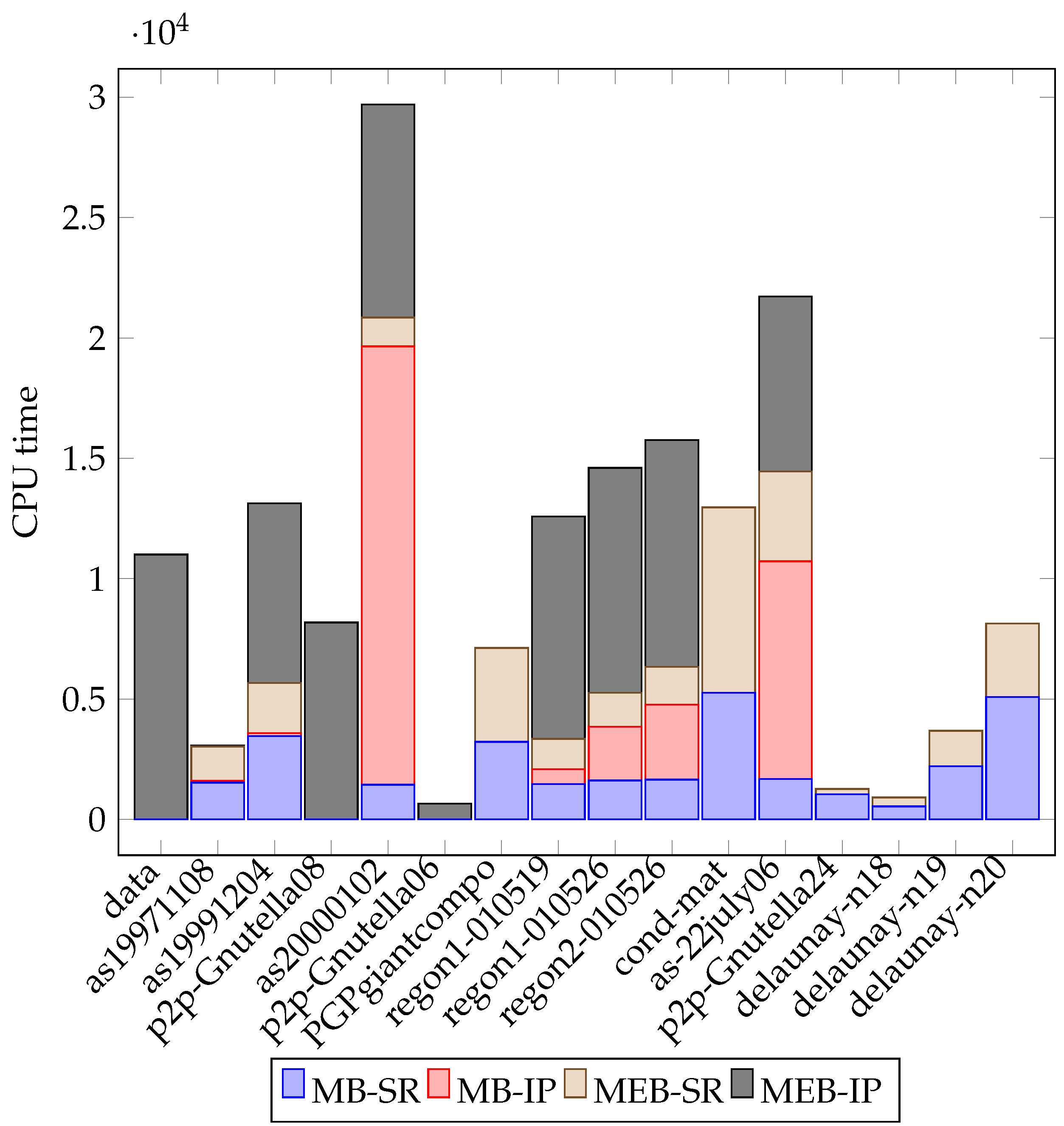
The CPU times taken by the scale reduction and IP steps of the exact approaches are illustrated in Figure 3 for 16 instances for which at least one of the four times (scale reduction for MB (MB-SR), IP solution for MB (MB-IP), scale reduction for MEB (MEB-SR), or IP solution for MB (MEB-IP)) exceeded 500 s. It can be seen that for 7 of these instances MEB-IP takes the longest, while MB-IP is the most time-consuming step for 2 more instances. The scale reduction techniques dominate the CPU time taken for the remaining 7 instances. Not surprisingly, the construction heuristic yielded optimal solutions for both the MB and MEB problems for 5 of these 7 instances, and was just short of optimum by 1 unit in the remaining two cases. For all these cases, the scale reduction procedure outputs a small residual graph that is easily handled by CPLEX.
It should be noted that the lower bound heuristic yielded optimal solution in most cases (23 and 20 out of 33 instances for the MB and MEB problems, respectively) and close to optimal solution in most of the remaining cases. This shows that the optimal bicliques tend to have a star structure and can often be found by analyzing the neighborhoods of individual vertices. The only two exceptions were “p2p-Gnutella06” and “p2p-Gnutella05” networks. The optimal MEB solutions for these instances had parts consisting of 23 and 6 vertices (yielding edges) and 46 and 2 vertices ( edges), respectively. Observe that despite a relatively large gap between the optimal objective value and the heuristic lower bound, the combination of the scale reduction and the IP-based approach was quite effective in finding optimal solution for both of these instances.
On the one hand, the observation that the optimal induced bicliques in real-life networks often correspond to star graphs can be used as yet another evidence of “global structural imbalance” in the so-called scale-free networks, which typically have a few high degree, and a large number of low-degree vertices. On the other hand, this motivates using bipartite and multipartite versions of clique relaxation models, such as s-plexes, s-defective cliques, and -quasicliques, which allow some missing edges between the parts and hence are less restrictive [43].
5. Conclusions
In this paper, we proposed a scale reduction technique for the MB and MEB problems, which can be used to expand the applicability of exact algorithms for this problem to larger instances. Through experiments with 33 real-life instances with the number of vertices ranging from 198 to 1,048,576, we have shown that the proposed method is very effective in reducing the considered instances to scales that can be handled by modern mixed integer programming (MIP) solvers. To further improve the IP solution time, one could perform a polyhedral study, explore and exploit the symmetries in the IP formulations, as well as take advantage of the high-quality heuristic solutions for warm-starting the MIP solvers. In addition, the proposed scale-reduction schemes with values high enough to yield the empty edge set in the residual graph could be used to obtain upper bounds on the MB and MEB size, as it was successfully done in [32] for the maximum clique problem.
In terms of the structure of the obtained optimal solutions, we observe that oftentimes optimal bicliques in real-life networks induce star subgraphs, which, on the one hand can be thought of as a global structural characteristic of scale-free networks, but on the other hand, may make one question the practicality of searching for maximum bicliques in the context of complex network analysis, where the instances are typically very sparse. These models may be more practical on denser networks, however, the proposed scale reduction technique will not be applicable in this case, calling for alternative solution methods, such as a combinatorial branch-and-bound method similar to RDS [29,44]. As noted above, RDS is not directly applicable due to the lack of heredity property, however, it can be modified to address the cases when heredity is violated. Other, more practical alternatives of bicliques that would be interesting to consider in future research are bipartite and multipartite versions of clique relaxations [43].
Acknowledgments
The authors thank the three anonymous reviewers for their very proficient and helpful suggestions. Partial support of the last author by NSF grant CMMI-1538493 is gratefully acknowledged. No funds were received for covering the costs to publish in open access.
Author Contributions
Shahram Shahinpour made major contributions to all aspects of this work, including the development, analysis and implementation of the algorithms as well as writing the manuscript. Shirin Shirvani participated in developing the computer codes and running the numerical experiments for the final version. Zeynep Ertem developed the initial implementation of the branch and bound approach and prepared the first version of the manuscript. Sergiy Butenko proposed the subject of investigation, supervised the efforts of all the co-authors, and prepared the final version of the paper.
Conflicts of Interest
The authors declare no conflict of interest. The funding sponsors had no role in the design of the study; in the collection, analyses, or interpretation of data; in the writing of the manuscript, and in the decision to publish the results.
Abbreviations
The following abbreviations are used in this manuscript:
| IP | integer programming |
| MIP | mixed integer programming |
| MB | maximum biclique |
| MEB | maximum edge biclique |
| RDS | Russian Doll Search |
References
- Gagneur, J.; Krause, R.; Bouwmeester, T.; Casari, G. Modular decomposition of protein-protein interaction networks. Genome Biol. 2004, 5, R57. [Google Scholar] [CrossRef] [PubMed] [Green Version]
- Jeong, H.; Mason, S.; Barabási, A.; Oltvai, Z.N. Lethality and certainty in protein networks. Nature 2001, 411, 41–42. [Google Scholar] [CrossRef] [PubMed]
- Spirin, V.; Mirny, L.A. Protein complexes and functional modules in molecular networks. Proc. Natl. Acad. Sci. USA 2003, 100, 12123–12128. [Google Scholar] [CrossRef] [PubMed]
- Madeira, S.C.; Oliveira, A.L. Biclustering Algorithms for Biological Data Analysis: A Survey. IEEE/ACM Trans. Comput. Biol. Bioinform. 2004, 1, 24–45. [Google Scholar] [CrossRef] [PubMed]
- Nussbaum, D.; Pu, S.; Sack, J.; Uno, T.; Zarrabi-Zadeh, H. Finding maximum edge bicliques in convex bipartite graphs. Algorithmica 2012, 64, 311–325. [Google Scholar] [CrossRef]
- Faloutsos, M.; Faloutsos, P.; Faloutsos, C. On power-law relationships of the Internet topology. In Proceedings of the ACM-SIGCOMM Conference on Applications, Technologies, Architectures, and Protocols for Computer Communication, Cambridge, MA, USA, 30 August–3 September 1999; pp. 251–262. [Google Scholar]
- Pastor-Satorras, R.; Vazquez, A.; Vespignani, A. Dynamical and correlation properties of the Internet. Phys. Rev. Lett. 2001, 87, 258701. [Google Scholar] [CrossRef] [PubMed]
- Acuña, V.; Ferreira, C.; Freire, A.; Moreno, E. Solving the maximum edge biclique packing problem on unbalanced bipartite graphs. Discrete Appl. Math. 2014, 164, 2–12. [Google Scholar] [CrossRef]
- Amilhastre, J.; Vilarem, M.; Janssen, P. Complexity of minimum biclique cover and minimum biclique decomposition for bipartite domino-free graphs. Discrete Appl. Math. 1998, 86, 125–144. [Google Scholar] [CrossRef]
- Cheng, Y.; Church, G. Biclustering of expression data. In Proceedings of the 8th International Conference on Intelligent Systems for Molecular Biology, La Jolla, CA, USA, 19–23 August 2000; pp. 93–100. [Google Scholar]
- Dawande, M.; Keskinocak, P.; Swaminathan, J.; Tayur, S. On Bipartite and Multipartite Clique Problems. J. Algorithms 2001, 41, 388–403. [Google Scholar] [CrossRef]
- Kumar, R.; Raghavan, P.; Rajagopalan, S.; Tomkins, A. Trawling the Web for Emerging Cyber-Communities. In Proceedings of the 8th international conference on World Wide Web, Toronto, ON, Canada, 11–14 May 1999; pp. 1481–1493. [Google Scholar]
- Liu, G.; Sim, K.; Li, J. Efficient Mining of Large Maximal Bicliques. In Proceedings of the International Conference on Data Warehousing and Knowledge Discovery, Krakow, Poland, 4–8 September 2006; Springer: Berlin/Heidelberg, Germany, 2006; Volume 4081, pp. 437–448. [Google Scholar]
- Sanderson, M.J.; Driskell, A.C.; Ree, R.H.; Eulenstein, O.; Langley, S. Obtaining maximal concatenated phylogenetic data sets from large sequence databases. Mol. Biol. Evol. 2003, 20, 1036–1042. [Google Scholar] [CrossRef] [PubMed]
- Alexe, G.; Alexe, S.; Crama, Y.; Foldes, S.; Hammer, P.L.; Simeone, B. Consensus algorithms for the generation of all maximal bicliques. Discrete Appl. Math. 2004, 145, 11–21. [Google Scholar] [CrossRef]
- Gély, A.; Nourine, L.; Sadi, B. Enumeration aspects of maximal cliques and bicliques. Discrete Appl. Math. 2009, 157, 1447–1459. [Google Scholar] [CrossRef]
- Mukherjee, A.P.; Tirthapura, S. Enumerating maximal bicliques from a large graph using MapReduce. In Proceedings of the 2014 IEEE International Congress on Big Data, Anchorage, AK, USA, 27 June–2 July 2014; pp. 707–716. [Google Scholar]
- Eppstein, D. Arboricity and bipartite subgraph listing algorithms. Inf. Process. Lett. 1994, 51, 207–211. [Google Scholar] [CrossRef]
- McCreesh, C.; Prosser, P. An exact branch and bound algorithm with symmetry breaking for the maximum balanced induced biclique problem. In Proceedings of the Integration of AI and OR Techniques in Constraint Programming: 11th International Conference, CPAIOR 2014, Cork, Ireland, 19–23 May 2014; Simonis, H., Ed.; Springer International Publishing: Cham, Switzerland, 2014; pp. 226–234. [Google Scholar]
- Binkele-Raible, D.; Fernau, H.; Gaspers, S.; Liedloff, M. Exact exponential-time algorithms for finding bicliques. Inf. Process. Lett. 2010, 111, 64–67. [Google Scholar] [CrossRef]
- Hochbaum, D.S. Approximating clique and biclique problems. J. Algorithms 1998, 29, 174–200. [Google Scholar] [CrossRef]
- Sim, K.; Li, J.; Gopalkrishnan, V.; Liu, G. Mining Maximal Quasi-Bicliques to Co-Cluster Stocks and Financial Ratios for Value Investment. In Proceedings of the Sixth International Conference on Data Mining (ICDM’06), Hong Kong, China, 18–22 December 2006; pp. 1059–1063. [Google Scholar]
- Maulik, U.; Mukhopadhyay, A.; Bhattacharyya, M.; Kaderali, L.; Brors, B.; Bandyopadhyay, S.; Eils, R. Mining Quasi-Bicliques from HIV-1-Human Protein Interaction Network: A Multiobjective Biclustering Approach. IEEE/ACM Trans. Comput. Biol. Bioinform. 2013, 10, 423–435. [Google Scholar] [CrossRef] [PubMed]
- Ganter, B.; Wille, R. Formale Begriffsanalyse-Mathematische Grundlagen; Springer: New York, NY, USA, 1996. [Google Scholar]
- Peeters, R. The maximum edge biclique problem is NP-complete. Discrete Appl. Math. 2003, 131, 651–654. [Google Scholar] [CrossRef]
- Ambühl, C.; Mastrolilli, M.; Svensson, O. Inapproximability results for maximum edge biclique, minimum linear arrangement, and sparsest cut. SIAM J. Comput. 2011, 40, 567–596. [Google Scholar] [CrossRef]
- Tan, J. Inapproximability of Maximum Weighted Edge Biclique and Its Applications. In Proceedings of the 5th International Conference on Theory and Application of Models of Computation, Xi’an, China, 25–29 April 2008; Springer: Berlin/Heidelberg, Germany, 2008; pp. 282–293. [Google Scholar]
- Yannakakis, M. Node and edge-deletion NP-complete problems. In Proceedings of the Tenth Annual ACM Symposium on Theory of Computing, San Diego, CA, USA, 1–3 May 1987; ACM: New York, NY, USA, 1978; pp. 253–264. [Google Scholar]
- Trukhanov, S.; Balasubramaniam, C.; Balasundaram, B.; Butenko, S. Algorithms for detecting optimal hereditary structures in graphs, with application to clique relaxations. Comput. Optim. Appl. 2013, 56, 113–130. [Google Scholar] [CrossRef]
- Verfaillie, G.; Lemaitre, M.; Schiex, T. Russian doll search for solving constraint optimization problems. In Proceedings of the National Conference on Artificial Intelligence, Portland, OR, USA, 4–8 August 1996; pp. 181–187. [Google Scholar]
- Abello, J.; Pardalos, P.M.; Resende, M.G.C. On maximum clique problems in very large graphs. In External Memory Algorithms; American Mathematical Society: Boston, MA, USA, 1999; pp. 119–130. [Google Scholar]
- Verma, A.; Buchanan, A.; Butenko, S. Solving the maximum clique and vertex coloring problems on very large sparse networks. INFORMS J. Comput. 2015, 27, 164–177. [Google Scholar] [CrossRef]
- Strash, D. On the power of simple reductions for the maximum independent set problem. In Proceedings of the International Computing and Combinatorics Conference (COCOON 2016), Ho Chi Minh City, Vietnam, 2–4 August 2016; Dinh, T.N., Thai, M.T., Eds.; Springer: Cham, Switzerland, 2016; pp. 345–356. [Google Scholar]
- Akiba, T.; Iwata, Y. Branch-and-reduce exponential/FPT algorithms in practice: A case study of vertex cover. Theor. Comput. Sci. 2016, 609, 211–225. [Google Scholar] [CrossRef]
- Cygan, M.; Fomin, F.; Kowalik, L.; Lokshtanov, D.; Marx, D.; Pilipczuk, M.; Pilipczuk, M.; Saurabh, S. Parameterized Algorithms; Springer: Cham, Switzerland, 2015. [Google Scholar]
- Downey, R.G.; Fellows, M.R. Parameterized Complexity; Springer: Cham, Switzerland, 1999. [Google Scholar]
- Lin, B. The parameterized complexity of k-biclique. In Proceedings of the Twenty-Sixth Annual ACM-SIAM Symposium on Discrete Algorithms, San Diego, CA, USA, 4–6 January 2015; SIAM: Philadelphia, PA, USA, 2015; pp. 605–615. [Google Scholar]
- Feng, Q.; Zhou, Z.; Wang, J. Parameterized Algorithms for Maximum Edge Biclique and Related Problems. In Proceedings of the Frontiers in Algorithmics: 10th International Workshop, FAW 2016, Qingdao, China, 30 June 30–2 July 2016; Zhu, D., Bereg, S., Eds.; Springer International Publishing: Cham, Switzerland, 2016; pp. 75–83. [Google Scholar]
- Östergård, P.R.J. A fast algorithm for the maximum clique problem. Discrete Appl. Math. 2002, 120, 197–207. [Google Scholar] [CrossRef]
- Tomita, E.; Sutani, Y.; Higashi, T.; Takahashi, S.; Wakatsuki, M. A Simple and Faster Branch-and-Bound Algorithm for Finding a Maximum Clique. In Proceedings of the WALCOM: Algorithms and Computation: 4th International Workshop, WALCOM 2010, Dhaka, Bangladesh, 10–12 February 2010; Rahman, M.S., Fujita, S., Eds.; Springer: Berlin/Heidelberg, Germany, 2010; pp. 191–203. [Google Scholar]
- SNAP. Stanford Large Network Dataset Collection. 2012. Available online: http://snap.stanford.edu/data/ (accessed on 20 May 2017).
- DIMACS. Graph Partitioning and Graph Clustering: Tenth DIMACS Implementation Challenge. 2012. Available online: http://cc.gatech.edu/dimacs10/ (accessed on 20 May 2017).
- Pattillo, J.; Youssef, N.; Butenko, S. On clique relaxation models in network analysis. Eur. J. Oper. Res. 2013, 226, 9–18. [Google Scholar] [CrossRef]
- Gschwind, T.; Irnich, S.; Podlinski, I. Maximum weight relaxed cliques and Russian Doll Search revisited. Discrete Appl. Math. 2017. (in press) [Google Scholar] [CrossRef]
Figure 1.
Graph the induced subgraphs and for (see Example 1).
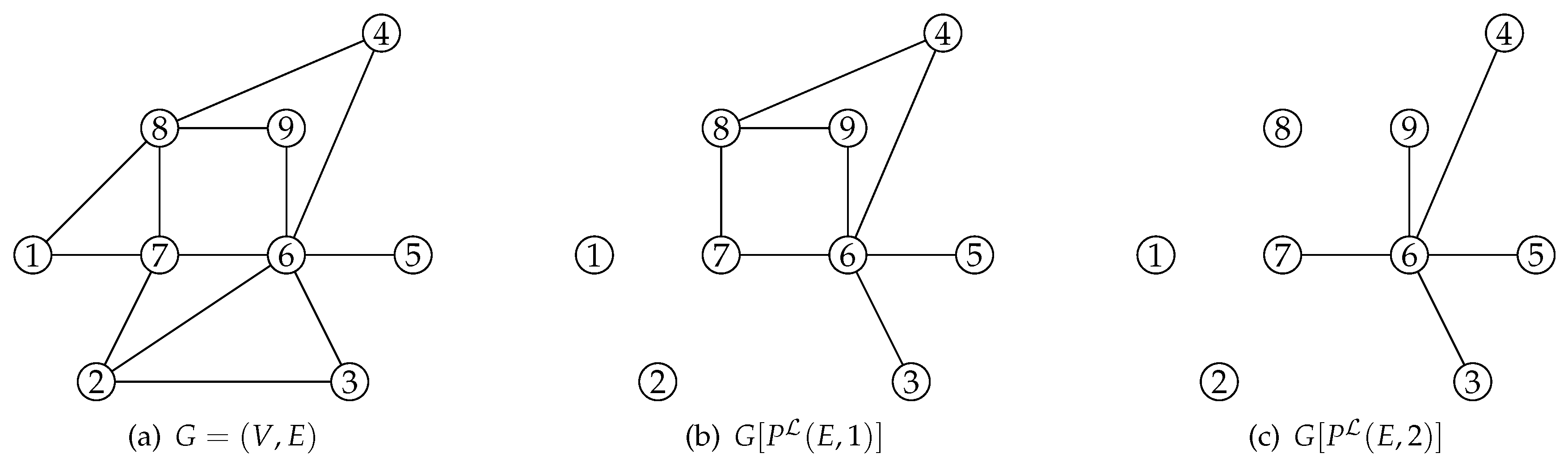
Figure 2.
Graph and the induced subgraph for and (see Example 2).
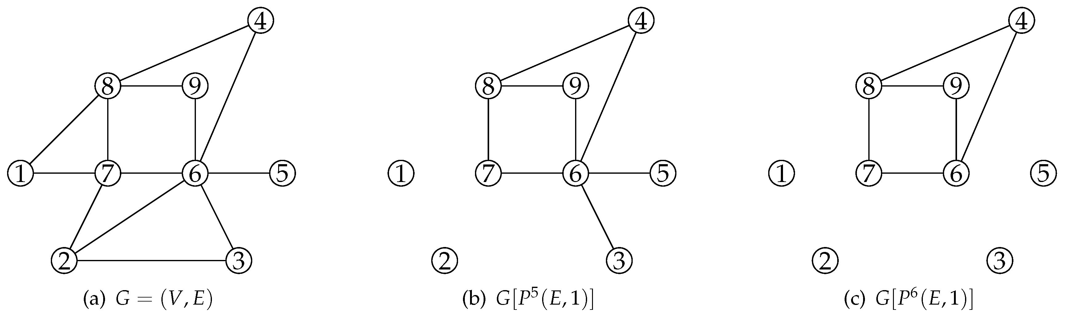
Figure 3.
Illustration of the CPU times used by the scale reduction and the IP solution for the MB problem (MB-SR and MB-IP, respectively) and for the MEB problems (MEB-SR and MEB-IP, respectively). The respective CPU times are plotted for all the tested instances for which at least one of the four times exceeded 500 s.

Table 1.
Computational results for the MB problem on instances from DIMACS Clustering challenge and Stanford Large Network Dataset Collection (SNAP) dataset.
Table 1.
Computational results for the MB problem on instances from DIMACS Clustering challenge and Stanford Large Network Dataset Collection (SNAP) dataset.
| Graph | LB | SR-CPU(s) | Opt. Obj. | CPU (s) | ||||
|---|---|---|---|---|---|---|---|---|
| jazz | 198 | 2742 | 18 | 85 | 704 | 0.44 | 20 | 0.67 |
| 1133 | 5451 | 34 | 35 | 35 | 0.61 | 34 | 0.64 | |
| netscience | 1589 | 2742 | 16 | 26 | 42 | 0.02 | 16 | 0.03 |
| add20 | 2395 | 7462 | 30 | 68 | 186 | 464.66 | 30 | 464.73 |
| data | 2851 | 15,093 | 8 | 41 | 99 | 1.09 | 8 | 1.36 |
| as19971108 | 3015 | 5347 | 540 | 583 | 740 | 1531.77 | 540 | 1602.59 |
| add32 | 4960 | 9462 | 16 | 66 | 108 | 0.17 | 16 | 0.42 |
| CA-GrQC | 5242 | 14,490 | 29 | 35 | 41 | 0.39 | 29 | 0.42 |
| as19991204 | 6296 | 12,830 | 1294 | 1407 | 2234 | 3461.69 | 1294 | 3582.89 |
| p2p-Gnutella08 | 6301 | 20,777 | 88 | 88 | 87 | 1.36 | 88 | 1.48 |
| as20000102 | 6474 | 13,233 | 1338 | 1454 | 2430 | 1440.82 | 1340 | 19,645.00 |
| p2p-Gnutella09 | 8114 | 26,013 | 98 | 98 | 97 | 1.09 | 98 | 1.47 |
| hep-th | 8361 | 15,751 | 22 | 81 | 151 | 0.40 | 23 | 0.66 |
| p2p-Gnutella06 | 8717 | 31,525 | 104 | 113 | 121 | 0.21 | 104 | 0.44 |
| p2p-Gnutella05 | 8846 | 31,839 | 87 | 88 | 88 | 0.76 | 87 | 1.11 |
| CA-HepTH | 9877 | 25,973 | 32 | 43 | 59 | 4.18 | 32 | 4.42 |
| PGPgiantcompo | 10,680 | 24,316 | 105 | 114 | 122 | 3223.57 | 105 | 3223.85 |
| p2p-Gnutella04 | 10,876 | 39,994 | 97 | 100 | 102 | 0.12 | 97 | 0.42 |
| oregon1-010519 | 11,051 | 22,724 | 2203 | 2384 | 4289 | 1466.45 | 2207 | 2085.01 |
| oregon1-010526 | 11,173 | 23,409 | 2199 | 2385 | 4308 | 1619.41 | 2203 | 3852.24 |
| oregon2-010526 | 11,460 | 16,365 | 2230 | 2428 | 4676 | 1652.65 | 2234 | 4762.25 |
| cond-mat | 16,726 | 47,594 | 41 | 55 | 72 | 5257.99 | 41 | 5258.05 |
| p2p-Gnutella25 | 22,687 | 54,705 | 64 | 66 | 67 | 0.22 | 64 | 0.33 |
| as-22july06 | 22,963 | 48,436 | 2243 | 2387 | 4125 | 1678.23 | 2245 | 10,722.34 |
| p2p-Gnutella24 | 26,518 | 65,369 | 304 | 356 | 426 | 1040.93 | 304 | 1043.72 |
| p2p-Gnutella30 | 36,682 | 88,328 | 54 | 54 | 53 | 0.59 | 54 | 0.70 |
| p2p-Gnutella31 | 62,586 | 147,892 | 90 | 95 | 100 | 0.41 | 90 | 0.70 |
| delaunay-n14 | 16,384 | 49,122 | 9 | 26 | 39 | 4.15 | 9 | 4.23 |
| delaunay-n16 | 65,536 | 196,575 | 9 | 18 | 34 | 61.05 | 9 | 61.13 |
| delaunay-n17 | 131,072 | 393,176 | 9 | 67 | 123 | 243.29 | 10 | 244.00 |
| delaunay-n18 | 262,144 | 786,396 | 11 | 65 | 123 | 541.73 | 12 | 542.29 |
| delaunay-n19 | 524,288 | 1,572,823 | 11 | 54 | 92 | 2205.50 | 11 | 2206.09 |
| delaunay-n20 | 1,048,576 | 3,145,686 | 12 | 24 | 45 | 5086.75 | 13 | 5087.06 |
Table 2.
Computational results for the MEB problem on instances from DIMACS Clustering challenge and SNAP dataset.
Table 2.
Computational results for the MEB problem on instances from DIMACS Clustering challenge and SNAP dataset.
| Graph | LB | SR-CPU(s) | Opt. Obj. | CPU (s) | ||||
|---|---|---|---|---|---|---|---|---|
| jazz | 198 | 2742 | 17 | 85 | 704 | 0.67 | 19 | 2.67 |
| 1133 | 5451 | 33 | 35 | 35 | 1.42 | 33 | 1.45 | |
| netscience | 1589 | 2742 | 15 | 26 | 42 | 0.01 | 15 | 0.03 |
| add20 | 2395 | 7462 | 29 | 68 | 186 | 306.95 | 29 | 307.45 |
| data | 2851 | 15,093 | 7 | 1944 | 11,290 | 0.78 | - | >11,000 |
| as19971108 | 3015 | 5347 | 539 | 583 | 740 | 1430.57 | 539 | 1462.28 |
| add32 | 4960 | 9462 | 15 | 66 | 108 | 0.17 | 15 | 0.89 |
| CA-GrQC | 5242 | 14,490 | 28 | 35 | 41 | 0.47 | 28 | 0.51 |
| as19991204 | 6296 | 12,830 | 1293 | 1407 | 2234 | 2081.83 | 1293 | 9542.64 |
| p2p-Gnutella08 | 6301 | 20,777 | 87 | 448 | 3194 | 9.19 | 87 | 8177.89 |
| as20000102 | 6474 | 13,233 | 1337 | 1454 | 2430 | 1201.03 | 1339 | 10,044.40 |
| p2p-Gnutella09 | 8114 | 26,013 | 97 | 98 | 97 | 12.37 | 97 | 12.51 |
| hep-th | 8361 | 15,751 | 21 | 81 | 151 | 0.50 | 22 | 1.26 |
| p2p-Gnutella06 | 8717 | 31,525 | 103 | 305 | 1283 | 2.53 | 138 | 654.47 |
| p2p-Gnutella05 | 8846 | 31,839 | 86 | 136 | 203 | 5.74 | 92 | 8.38 |
| CA-HepTH | 9877 | 25,973 | 31 | 43 | 59 | 6.19 | 31 | 6.51 |
| PGPgiantcompo | 10,680 | 24,316 | 104 | 114 | 122 | 3899.91 | 104 | 3900.27 |
| p2p-Gnutella04 | 10,876 | 39,994 | 96 | 100 | 102 | 0.56 | 96 | 0.78 |
| oregon1-010519 | 11,051 | 22,724 | 2202 | 2384 | 4289 | 1262.38 | 2206 | 10,494.20 |
| oregon1-010526 | 11,174 | 23,409 | 2198 | 2385 | 4308 | 1415.75 | 2202 | 10,750.50 |
| oregon2-010526 | 11,460 | 16,365 | 2229 | 2428 | 4676 | 1579.16 | - | >11,000 |
| cond-mat | 16,726 | 47,594 | 40 | 55 | 72 | 7703.95 | 40 | 7704.02 |
| p2p-Gnutella25 | 22,687 | 54,705 | 63 | 66 | 67 | 0.31 | 63 | 0.44 |
| as-22july06 | 22,963 | 48,436 | 2242 | 2387 | 4125 | 3735.30 | - | >11,000 |
| p2p-Gnutella24 | 26,518 | 65,369 | 303 | 356 | 426 | 220.50 | 303 | 225.52 |
| p2p-Gnutella30 | 36,682 | 88,328 | 53 | 54 | 53 | 2.06 | 53 | 2.12 |
| p2p-Gnutella31 | 62,586 | 147,892 | 89 | 95 | 100 | 0.98 | 89 | 1.30 |
| delaunay-n14 | 16,384 | 49,122 | 8 | 26 | 39 | 5.57 | 8 | 5.70 |
| delaunay-n16 | 65,536 | 196,575 | 8 | 18 | 34 | 80.41 | 8 | 80.54 |
| delaunay-n17 | 131,072 | 393,176 | 8 | 67 | 123 | 315.68 | 9 | 316.55 |
| delaunay-n18 | 262,144 | 786,396 | 10 | 65 | 123 | 373.68 | 11 | 374.53 |
| delaunay-n19 | 524,288 | 1,572,823 | 10 | 54 | 92 | 1478.44 | 10 | 1479.16 |
| delaunay-n20 | 1,048,576 | 3,145,686 | 11 | 24 | 45 | 3044.67 | 12 | 3045.02 |
© 2017 by the authors. Licensee MDPI, Basel, Switzerland. This article is an open access article distributed under the terms and conditions of the Creative Commons Attribution (CC BY) license (http://creativecommons.org/licenses/by/4.0/).
Share and Cite
MDPI and ACS Style
Shahinpour, S.; Shirvani, S.; Ertem, Z.; Butenko, S. Scale Reduction Techniques for Computing Maximum Induced Bicliques. Algorithms 2017, 10, 113. https://doi.org/10.3390/a10040113
AMA Style
Shahinpour S, Shirvani S, Ertem Z, Butenko S. Scale Reduction Techniques for Computing Maximum Induced Bicliques. Algorithms. 2017; 10(4):113. https://doi.org/10.3390/a10040113
Chicago/Turabian StyleShahinpour, Shahram, Shirin Shirvani, Zeynep Ertem, and Sergiy Butenko. 2017. "Scale Reduction Techniques for Computing Maximum Induced Bicliques" Algorithms 10, no. 4: 113. https://doi.org/10.3390/a10040113
Note that from the first issue of 2016, this journal uses article numbers instead of page numbers. See further details here.