Variable Selection in Time Series Forecasting Using Random Forests


Department of Water Resources and Environmental Engineering, School of Civil Engineering, National Technical University of Athens, Iroon Polytechniou 5, 157 80 Zografou, Greece
*
Author to whom correspondence should be addressed.
Algorithms 2017, 10(4), 114; https://doi.org/10.3390/a10040114
Submission received: 29 July 2017
/
Revised: 25 September 2017
/
Accepted: 1 October 2017
/
Published: 4 October 2017
(This article belongs to the Special Issue Computational Intelligence and Nature-Inspired Algorithms for Real-World Data Analytics and Pattern Recognition)
Abstract
:Time series forecasting using machine learning algorithms has gained popularity recently. Random forest is a machine learning algorithm implemented in time series forecasting; however, most of its forecasting properties have remained unexplored. Here we focus on assessing the performance of random forests in one-step forecasting using two large datasets of short time series with the aim to suggest an optimal set of predictor variables. Furthermore, we compare its performance to benchmarking methods. The first dataset is composed by 16,000 simulated time series from a variety of Autoregressive Fractionally Integrated Moving Average (ARFIMA) models. The second dataset consists of 135 mean annual temperature time series. The highest predictive performance of RF is observed when using a low number of recent lagged predictor variables. This outcome could be useful in relevant future applications, with the prospect to achieve higher predictive accuracy.
1. Introduction
1.1. Time Series Forecasting and Random Forests
The use of machine learning algorithms in predictive modelling (see for the definition [1]) and in the specific case of time series forecasting has increased considerably recently [2]. Relevant applications can be found in the review papers [3,4,5,6].
Time series forecasting can be classified into two categories according to the forecast horizon, i.e., one-step and multi-step forecasting [2,7]. The one-step forecasting (examined here) is useful in single applications, e.g., in assessing forecasting methods using simulations [8], engineering forecasting [9,10], environmental forecasting [11,12], and financial forecasting [13,14,15,16,17]. Furthermore, the recursive and the DiRec multi-step forecasting strategies depend on the one-step forecasting. In particular, one-step ahead forecasts are used in the recursive strategy, while in each step the forecasted value of the previous step is used as additional input, without changing the forecasting model. The DiRec strategy combines the recursive strategy, but the forecasting model changes in every step [7].
The random forest (RF) is a machine learning algorithm introduced in [18], which can be used for classification and regression. It is popular because it can be applied to a wide range of prediction problems, it has a few parameters to tune, it is simple to use, it has been successfully applied to many practical problems and it can deal with small sample sizes, high-dimensional feature spaces, and complex data structures [19,20]. A review and a simple presentation of the RF algorithm can be found in [20,21,22]. Regression using RF can be implemented for time series forecasting purposes. Representative applications can be found in many scientific fields including these of engineering [23,24], environmental and geophysical sciences [25,26,27], financial studies [28,29], and medicine [30], with varying performance. Furthermore, small datasets are used in these applications; therefore, the results cannot be generalized.
The performance of the RF algorithm depends on the tuning of its parameters and the variable selection (also known as feature selection). Procedures for estimating the optimal set of parameters are proposed in several studies. These procedures consider the performance of the algorithm depending on the selected variables [22,31], the number of trees [32,33], the number of possible directions for splitting at each node of each tree [20,34] (p. 199), and the number of examples in each cell, below which the cell is not split [20,35]. There are also some studies examining the RF properties in a theoretical context [19].
The performance of machine learning algorithms is usually assessed using single case studies. Sometimes large datasets composed of real-world studies are used for benchmarking and the comparison of several algorithms [7,36,37,38,39,40]. Moreover, [41] proposes the use of simulations as a considerable alternative. Respective applications can be found in [42,43].
1.2. A Framework to Assess the Performance of Random Forests in Time Series Forecasting
In usual regression problems, a sample consisting of observations of the dependent variable and the respective observations of the predictor variables is given. The regression model is trained using this sample. Prediction is then performed when new observations of the predictor variables are obtained. If we decide to use fewer predictor variables than that included in the sample, then the size of the training set does not change. Moreover, it is important that the inclusion of unimportant predictor variables does not seriously impact the predictive performance of RF, as indicated in [34] (p. 489). On the other hand, using RF for time series forecasting is not identical to the simple regression case. In this case, the role of the predictor variables is taken by previous values of the time series (lagged variables). Therefore, increasing the number of predictor variables, i.e., the selected lagged variables, inevitably results in reducing the length of the training set. Using fewer predictor variables instead may reduce the information obtained by the available knowledge of the temporal dependence.
The analytical computation of the performance is not attainable, due to the complexity of the RF algorithm [20]. Nevertheless, an empirical answer could be given in the context of a large experiment. Furthermore, in this simulation experiment the RF could be compared to benchmarking methods, whose performance is known a priori, theoretically. Here we perform a large simulation experiment, in which we use 16,000 simulated time series from a variety of Autoregressive Fractionally Integrated Moving Average (ARFIMA) models [44,45]. Similar studies using simulations from the family of ARFIMA models can be found in [46,47], although to a lesser extent and implementing different methods. Simulation studies are effectively complemented when integrated with case studies; consequently, we additionally apply the methods to a dataset of 135 mean annual instrumental temperatures from the dataset in [48]. The length of each simulated and observed time series is 101.
We compare the performance of five algorithms in forecasting the 101st value of each time series, when fitted to its first 100 values. The five algorithms implemented in the study are two naïve methods, an ARFIMA model, the theta method and the RF algorithm. The naïve methods usually perform well in predicting time series [37] and the ARFIMA processes are traditional methods which are frequently used for time series forecasting [45]. The theta method has been recently introduced and is also one of the most successful forecasting methods [49]. We use various versions of the RF algorithm with respect to the number of predictor variables, while the optimization of the parameter set is performed using methods proposed in [50,51]. The metrics used for the comparison are the mean absolute error (MAE), the mean squared error (MSE), the mean absolute percentage error (MAPE), and the linear regression coefficient. The analysis performed here regards time series simulated from stationary stochastic processes, while stationary models are also used to model the temperature time series.
1.3. Aim of the Study
The primary aim of our study is to investigate how the performance of RF is related to the variable selection in one-step forecasting of short time series. The proposed framework in Section 1.2 can help in providing an empirical answer to the problem of variable selection. In conclusion, it is shown that a low number of recent lagged variables performs better, highlighting the importance of the training set’s length. The RF algorithm is proven to be competent in time series forecasting, even though it has not exhibited the best performance in most of the examined cases. This does not imply that the RF are of little practical value. Instead, as has been shown in [12], there is not a universally best forecasting method, therefore, in practical applications we should use multiple methods for obtaining a good forecast. In such cases, we emphasize that appropriate methodologies for the optimization of the performance of each method should be used. Our contribution regards the optimization of the forecasting performance of the RF.
2. Methods and Data
In Section 2, we present the methods and data used in the present study. In particular, we present the definitions of the models used for simulation and testing, as well as the forecasting methods. Additionally, we present the temperature data, also used for the testing of the methods. The codes and data to reproduce the study are available as supplementary material (see Appendix A). The computations were performed using the R programming language [52].
2.1. Methods
2.1.1. Definition of ARMA and ARFIMA Models
Here, we provide the definitions of the autoregressive moving average (ARMA) and ARFIMA stochastic processes, while the reader is also referred to [45] (pp. 6–65, 489–494) for further information. A time series in discrete time is defined as a sequence of observations x1, x2, …, of a certain phenomenon, while the time t is stated as a subscript to each value xt. A time series can be modelled by a stochastic process. The latter is a sequence of random variables x1, x2, …. Random variables are underlined according to the notation used in [53].
Let us consider a stationary stochastic process of normally-distributed random variables. The mean μ of the stochastic process is defined by:
μ := E[xt],
The standard deviation function σ of the stochastic process is defined by:
σ := (Var[xt])0.5
The covariance function between xt and xt+k, γk of the stochastic process is defined by:
γk := E[(xt − μ)(xt+k − μ)]
The correlation function between xt and xt+k, ρk of the stochastic process is defined by:
ρk := γk/σ2
A normal stationary stochastic process {at} is called a white noise process, if it is a sequence of uncorrelated random variables. Let us consider hereinafter that the white noise is a variable with zero mean, unless mentioned otherwise, and standard deviation σa.
We define the stochastic process {yt} by:
yt := xt − μ
Let us consider the operator Β, which is defined by:
Bjxt = xt−j
Then the operator φp(B) is defined by:
φp(B) := (1 − φ1B − … − φpBp)
The stochastic process {xt} is an autoregressive AR(p) model, if:
which can be written in the following form:
φp(B)yt = at,
yt = φ1yt−1 + … + φpyt−p + at
Let us also consider the operator θq(B), which is defined by:
θq(B) := (1 + θ1B + … + θqBq)
The stochastic process {xt} is a moving average MA(q) model, if:
which can be written in the following form:
yt = θq(B) at,
yt = at + θ1at−1 + … + θqat−q
The stochastic process {xt} is an autoregressive moving average ARMA(p, q) model, if
which can be written in the following form:
φp(B)yt = θq(B)at,
yt = φ1yt−1 + … + φpyt−p + at + θ1at−1 + … + θqat−q
Let d ∊ (−0.5, 0.5). The stochastic process {xt} is an ARFΙMA(p, d, q), if
φp(B)(1 − B)dxt = θq(B)at
2.1.2. Simulation of ARMA and ARFIMA Models
2.1.3. Forecasting Using ARMA and ARFIMA Models
Here we present how we can use ARMA and ARFIMA models in one-step ahead time series forecasting. The specific applications of the forecasting methods are presented in Section 2.1.8. We consider a time series of n observations. Let us also consider a model fitted to the n observations and subsequently used to forecast xn+1. Let xn and ψ represent the last observation and the forecast of xn+1, respectively. The methods using ARMA and ARFIMA models can be used as benchmarks in the simulation experiments. In fact, these methods are expected to perform better than the rest, when applied to the synthetic time series, since the latter are simulated using ARMA or ARFIMA models (see Section 2.1.8). We examine two cases.
In the first case we assume that the time series are modelled by an ARMA(p, q), in which p and q are predefined, while the parameters must be estimated. We fit ARMA models to the data using the arima built in R function. During the implementation process, the values of p, q are set equal to the respective values used in the corresponding simulation experiment. The function applies the maximum likelihood method to estimate the values of the AR and MA parameters φ1, ..., φp, θ1, ..., θq of the models. We use the fitted ARMA model in forecast mode by implementing the predict built in R function [52].
In the second case, we assume that the time series can be modelled by an ARFΙMA(p, d, q) model with unknown parameters. We fit an ARFIMA model to the data using the arfima function of the R package forecast [55,56]. The values of p, d, q are estimated using the Akaike Information Criterion with a correction for finite sample sizes (AICc), with d ranging between −0.5 and 0.5. The function applies the maximum likelihood method to estimate the values of the AR and MA parameters φ1, ..., φp, θ1, ..., θq of the models. The order selection and parameter estimation procedures are explained, for example, in [57] (Chapter 8.6). We use the fitted ARFIMA model in forecast mode by implementing the forecast function of the forecast R package.
2.1.4. Forecasting Using Naïve Methods
We use two naïve forecasting methods, the last observation naïve and the average naïve, which are amongst the most commonly used benchmarks [57] (Chapter 2.3). The produced forecasts are given by (16) and (17) respectively:
ψ = xn
ψ = (x1 + … + xn)/n
The naïve methods presented here are benchmarks, because they are the simplest forecasting methods in terms of theoretical complexity and computational cost.
2.1.5. Forecasting Using the Theta Method
We implement a simple version of the theta forecasting method, which was introduced in [49], through the thetaf function of the R package forecast. Theta uses a given time series to create two or more auxiliary time series with different (modified) local curvatures with respect to the original, namely the “Theta-lines”. The latter are extrapolated separately and subsequently combined with equal weights to produce the forecast. The modification of the local curvatures is implemented using the “Theta-coefficient” θ, which is applied to the second differences of the time series.
The here adopted version uses two Theta-lines, for θ = 0 and θ = 2. This specific version performed well in the M3-Competition [37], while later [58] proved its equivalence to simple exponential smoothing (SES) with drift. For the exponential smoothing forecasting methods, and particularly for their implementation into a state space framework, the reader is referred to [57] (Chapter 7) and [59], respectively.
2.1.6. Random Forests
RF is a vague term [20]. Here we use the original RF algorithm introduced in [18]. In particular, we present the version of the algorithm used for regression. The specific version of the algorithm has been implemented in the randomForest R package [60]. The remainder of the section is largely reproduced from [20] with adaptations, while identical notation is used in [20,60]. The present Section is not intended to provide a detailed description of RF. The interested reader can find further details in [20], while the computations are reproducible (Appendix A).
We assume that the u is a random vector with k elements. The aim is to predict v by estimating the regression function:
given the fitting sample:
which are independent realizations of the random variable (u, v). Therefore, the aim is to construct an estimate ms of the function m.
m(u) = E[v|u = u]
Ss = ((u1, v1), …, (us, vs))
A random forest is a predictor constructed by growing M randomized regression trees. For the j-th tree in the family, the predicted value at u is denoted by ms(u; θj, Ss), where θ1, ..., θM are independent random variables, distributed as θ and independent of Ss. The random variable θ is used to resample the fitting set prior to the growing of individual trees and to select the successive directions for splitting. The prediction is then given by the average of the predicted values of all trees.
Before constructing each tree, bs observations are randomly chosen from the elements of u. These observations are used for growing the tree. At each cell of the tree, a split is performed by maximization of the CART-criterion (defined in [20]) by selecting mtry variables randomly among the k original ones, picking the best variable/split point among the mtry and splitting the node into two daughter nodes. The growing of the tree is stopped when each cell contains fewer than nodesize points.
The parameters used in RF are bs ∊ {1, …, s}, mtry ∊ {1, …, k}, nodesize ∊ {1, …, bs}, and M ∊ {1, 2, …}. In most studies, it is agreed that increasing the number of trees does not decrease the predictive performance; however, it results in an increase of the computational cost. Oshiro et al. [32] suggests a range between 64 and 128 trees in a forest based on experiments. Kuhn and Johnson [34] (p. 200) suggest using at least 1000 trees. Probst and Boulesteix [33] suggest that the highest performance gain is achieved when training 100 trees. In the present study, we use M = 500 trees.
The number of sampled data points in each tree and the number of examples in each cell below which the cell is not split are set equal to their default values in the randomForest R package, i.e., equal to the sample size and nodesize = 5, respectively. These are reported to be good values [20,35].
The parameter mtry is estimated during the validation phase by implementing the trainControl function of the R package caret [50,51]. The optimal mtry is found by using bootstrap resampling, i.e., randomly sampling the validation test with reselection (the size of the bootstrap sample must be equal to the size of the validation test), fitting the model in the bootstrap sample and measuring its performance in the remaining set, i.e., the data not selected by the bootstrap sampling. Twenty-five iterations are used in the resampling procedure. The optimal mtry is found by calculating the average performance of the fitted models, while the search for the optimal value of the parameter is performed in a grid. The root mean squared error (RMSE) is used to measure the performance. The optimal mtry minimizes the RMSE. Details on the theoretical background of the method can be found in [34] (pp. 72–73). The regression function of Equation (18) is defined by the model, which is fitted to the validation test using the optimal mtry value.
2.1.7. Time Series Forecasting Using Random Forests
Using RF for one-step time series forecasting is straightforward and similar to the way that RF can be used for regression. Let g be the function obtained from the training of RF, which will be used for forecasting xn+1, given x1, …, xn. If we use k lagged variables then the forecasted xn+1 is given by the following equation for t = n + 1:
xt = g(xt−1, …, xt−k), t = k + 1, …, n + 1
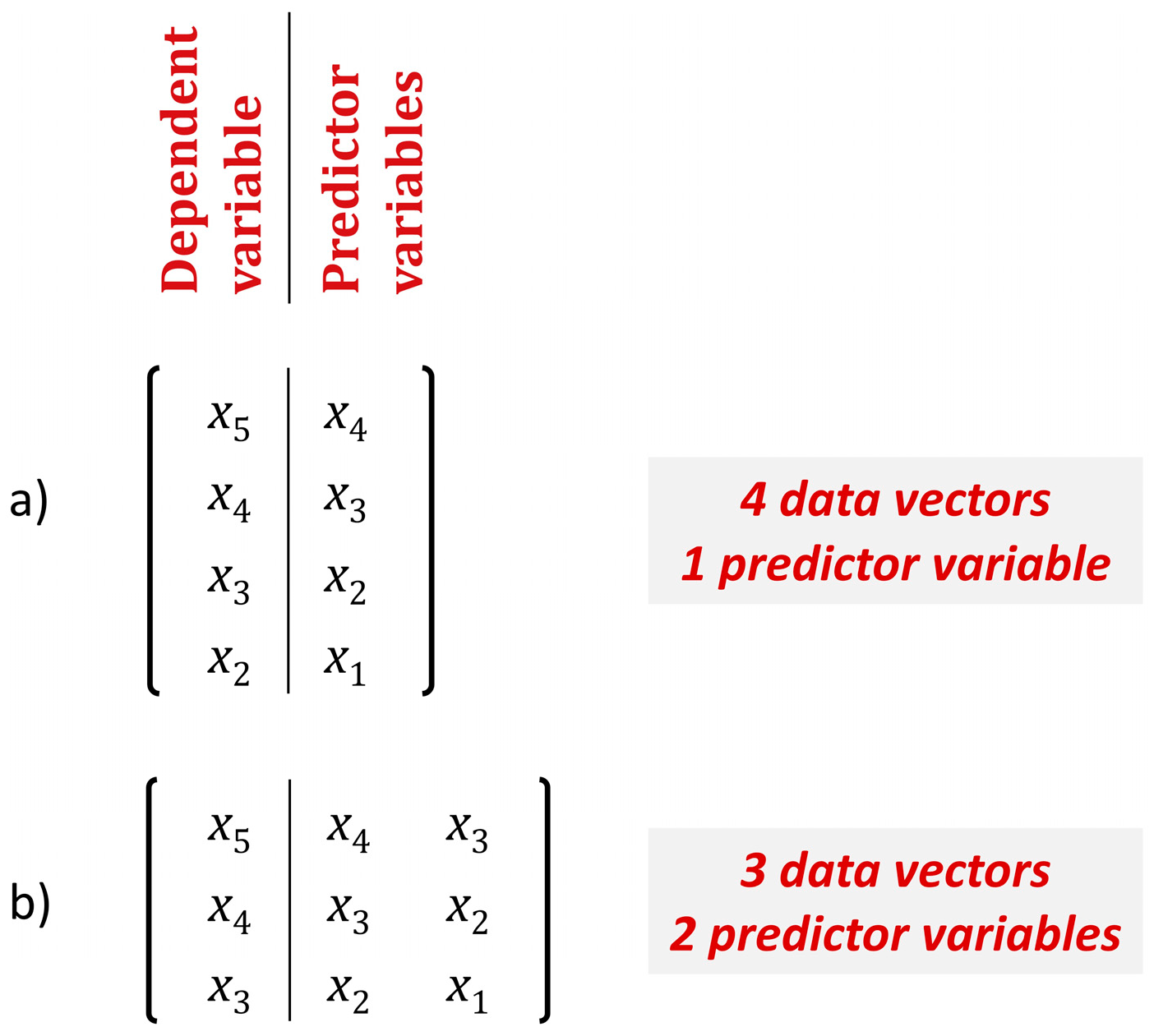
The function g is not in closed form, but can be obtained by training the RF algorithm using a training set of size n − k. In each sample of the fitting set the dependent variable is xt, for t = k + 1, …, n + 1, while the predictor variables are xt−1, …, xt−k. When the number of predictor variables k increases, the size of the training set n − k decreases (an example is presented in Figure 1). The training set, which includes n – k samples, is created using the CasesSeries function of the rminer R package [61,62]. Finally, the fitting is performed using the train function of the caret R package and the forecasted value of xn+1 is obtained using the predict function of the caret R package.
Kuhn and Johnson [34] (p. 463) defines the variable importance as the overall quantification of the relationship between the predictor variables and the predicted value. Here we use the first measure of variable importance in RF as defined in the randomForest R package [60]. From the training procedure using k predictor variables, we keep the variables with positive variable importance and define a new set of predictor variables, which includes these variables. Then we repeat the forecasting procedure. In this case, the size of the sample depends on the minimum index of the subset of predictor variables when forecasting xn+1, e.g., if the minimum index is n + 1 − k, then the training set is of size n − k. However, using fewer predictor variables decreases the computational cost.
2.1.8. Summary of the Methods
In Table 1, we summarize the methods presented in Section 2.1.3, Section 2.1.4, Section 2.1.5, Section 2.1.6 and Section 2.1.7. In Table 2, we present the category of data to which we apply each specific case of the ARMA and ARFIMA model based methods in Section 3. In Table 3, we present the 12 different variable selection procedures used by the RF algorithm.
2.1.9. Metrics
Here we define the metrics used in the comparisons. The error (E) is defined by:
E := ψ − xn+1
The absolute error (AE) is defined by:
AE := |ψ − xn+1|
The squared error (SE) is defined by:
SE := (ψ − xn+1)2
The percentage error (PE) is defined by:
PE := (ψ − xn+1)/xn+1
The absolute percentage error (APE) is defined by:
APE := |ψ − xn+1/xn+1|
The metrics defined in Equations (21)–(25) can be used for the assessment of the performance in single experiments. To assess the forecasting performance using a set of multiple simulations, the metrics must be summarized. Let N be the number of the conducted forecasting experiments. Let the serial number of each experiment i be stated as a subscript to each metric value Ei, AEi, SEi, PEi and APEi. Then, the mean of the errors (MoE) is defined by:
MoE := (E1 + … + EN)/N
The median of the errors (MdoE) is defined by:
MdoE := median(E1, …, EN)
The mean of the absolute errors (MoAE) is defined by:
MoAE := (AE1 + … + AEN)/N
The median of the absolute errors (MdoAE) is defined by:
MdoAE := median(AE1, …, AEN)
The mean of the squared errors (MoSE) is defined by:
MoSE := (SE1 + … + SEN)/N
The median of the squared errors (MdoSE) is defined by:
MdoSE := median(SE1, …, SEN)
The mean of the percentage errors (MoPE) is defined by:
MoPE := (PE1 + … + PEN)/N
The median of the percentage errors (MdoPE) is defined by:
MdoPE := median(PE1, …, PEN)
The mean of the absolute percentage errors (MoAPE) is defined by:
MoAPE := (APE1 + … + APEN)/N
The median of the absolute percentage errors (MdoAPE) is defined by:
MdoAPE := median(APE1, …, APEN)
The means and the medians can substantially differ when outliers are observed; therefore, they are both useful in the assessment of the forecasting performance. Another useful metric of the forecasting performance, when assessing multiple experiments simultaneously, is the slope of the regression. Let i also be stated as a subscript to each forecast ψi and its corresponding true value xn+1,i. The regression coefficient a (or slope of the regression) is estimated to measure the dependence of ψ1, …, ψN on xn+1,1, …, xn+1,N, when this dependence is expressed by the following linear regression model:
ψi = a xn+1,i + b
In Table 4, we present the range of the values of the metrics and their values when the forecast is perfect.
A discussion on the appropriateness of the metrics to measure the performance of the forecasting methods can be found in [57] (Chapter 2.5) and [63], while [64,65] extensively discuss metrics connected to the regression coefficient. Here we preferred to use the metrics of Table 4, due to their simplicity.
2.2. Data
Here we present the data used in the present study. We used two large datasets. The first was obtained from simulations from the models presented in Section 2.1.2. The second dataset is a set of observed annual temperatures.
2.2.1. Simulated Time Series
We used 16 models from the family of ARFIMA models presented in Section 2.1.1. Each model corresponds to a simulation experiment as presented in Table 5. Each simulation experiment includes 1000 simulated time series of size 101 from the models of Table 5.
2.2.2. Temperature Dataset
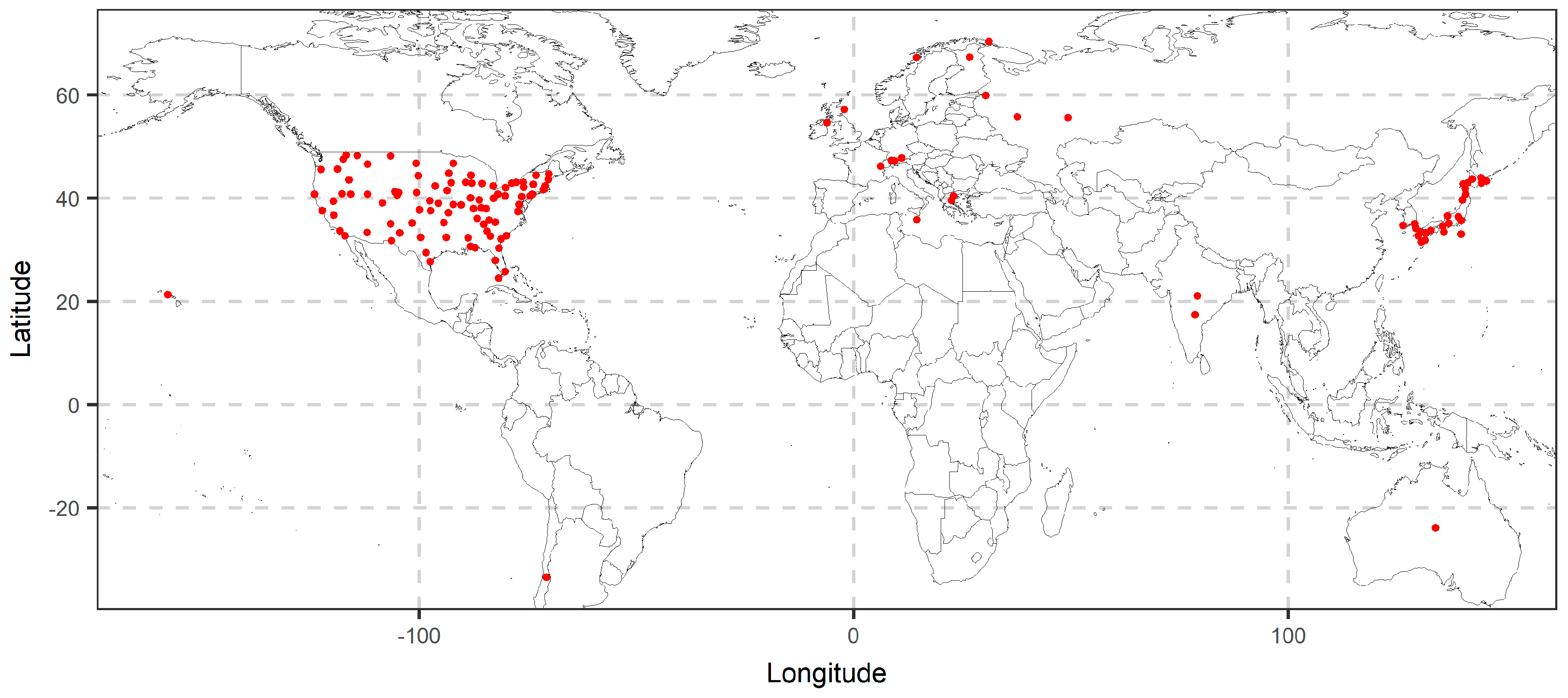
The real-world dataset includes 135 mean annual instrumental temperature time series extracted from the database of [48]. The database includes observed mean monthly temperatures. We extracted stations, which included mean monthly temperatures for the period 1916–2016, i.e., 101 years of observations. We discarded stations with missing data. We depict the 135 remaining stations in Figure 2. The stations cover a considerable part of the Earth’s surface, therefore, they can represent diverse behaviours observed in geophysical time series. The mean annual temperatures were obtained by averaging per year the monthly values.
3. Results
Here we present the results from the application of the methods to the data presented in Section 2. We use two datasets including time series of size 101. The two datasets include simulated time series and observed temperatures. The fitting is performed in the first 100 values of the time series, while the methods are compared in forecasting the 101st value. The application of the methods to specific datasets was presented in Section 2.1.8.
3.1. Simulations
We present the results from the application of the methods to the simulated time series. Each simulation experiment lasts 30 h, while the computation time for all the methods excluding RF is some minutes. In particular, we present the boxplots of the absolute errors and the errors. Furthermore, we present the medians of the absolute errors, medians of the squared errors and the regression coefficients. The rf methods were optimized by minimizing the RMSE, therefore, the most representative figures of their predictive performance are the ones presenting the squared errors. Given that the information presented by the boxplots of the squared errors (available in the supplementary information) is minimal, we mostly present here results related to the absolute errors of the forecasts. The two approaches yield equivalent results, as shown in the present sections. Additionally, the primary aim of the present study is the optimization of the predictive performance of the RF, therefore, the results of the methods described in Section 2, should be assessed using various methods. Detailed results for all the experiments can be found in the analysis.html file in Appendix A.
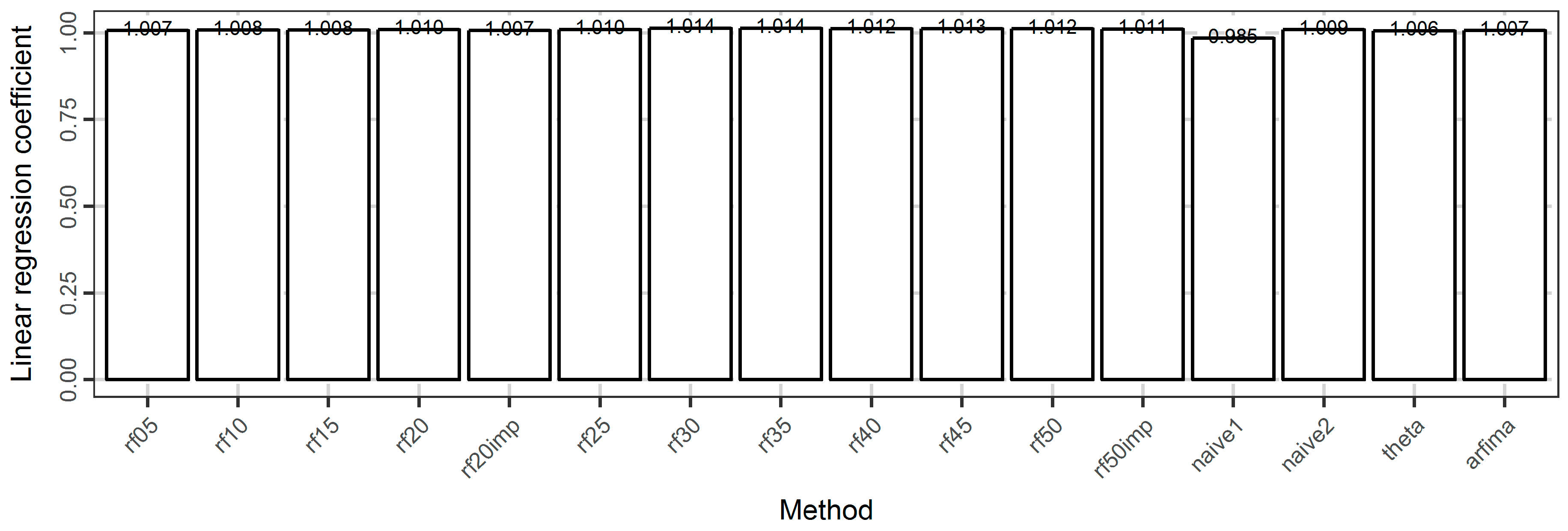
In Figure 3, we present a typical example in which we test the methods when applied to the 1000 time series simulated from the ARMA(1, 0) model with φ1 = 0.6. In this typical example, we observe that all methods perform similarly with respect to the absolute and squared errors. The rf30 method is the best amongst the rf methods, while arfima has the best performance and naïve2 has the worst performance. The arfima method is approximately 5% better than the best rf methods. The naïve1 and theta methods perform similarly to the best rf methods. The simplest rf method, i.e., rf1, performs well. In fact, its performance is comparable to the best rf methods, i.e., rf20imp, rf25, and rf30. Regarding the use of important variables, introduced with the rf20imp and the rf50imp methods, their performance is similar to that of the rf20 and rf50 methods, respectively.
When looking at the regression coefficients, the pattern of the performance of the methods is clear. The rf methods are better when using fewer predictor variables. The naïve1 method performs better than all methods, followed by the theta and arfima methods.
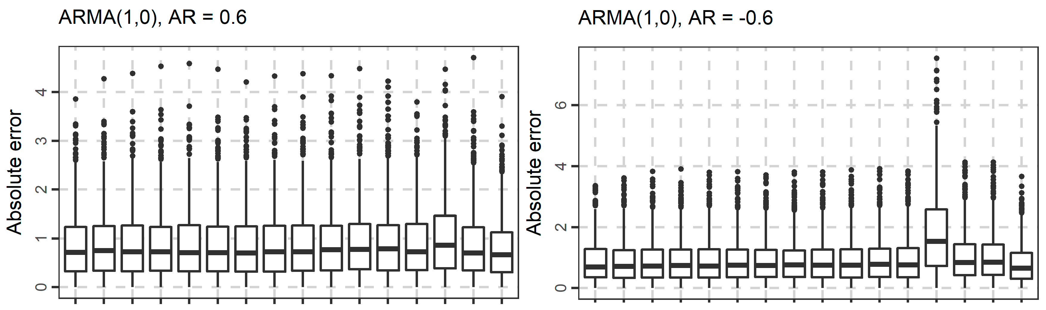
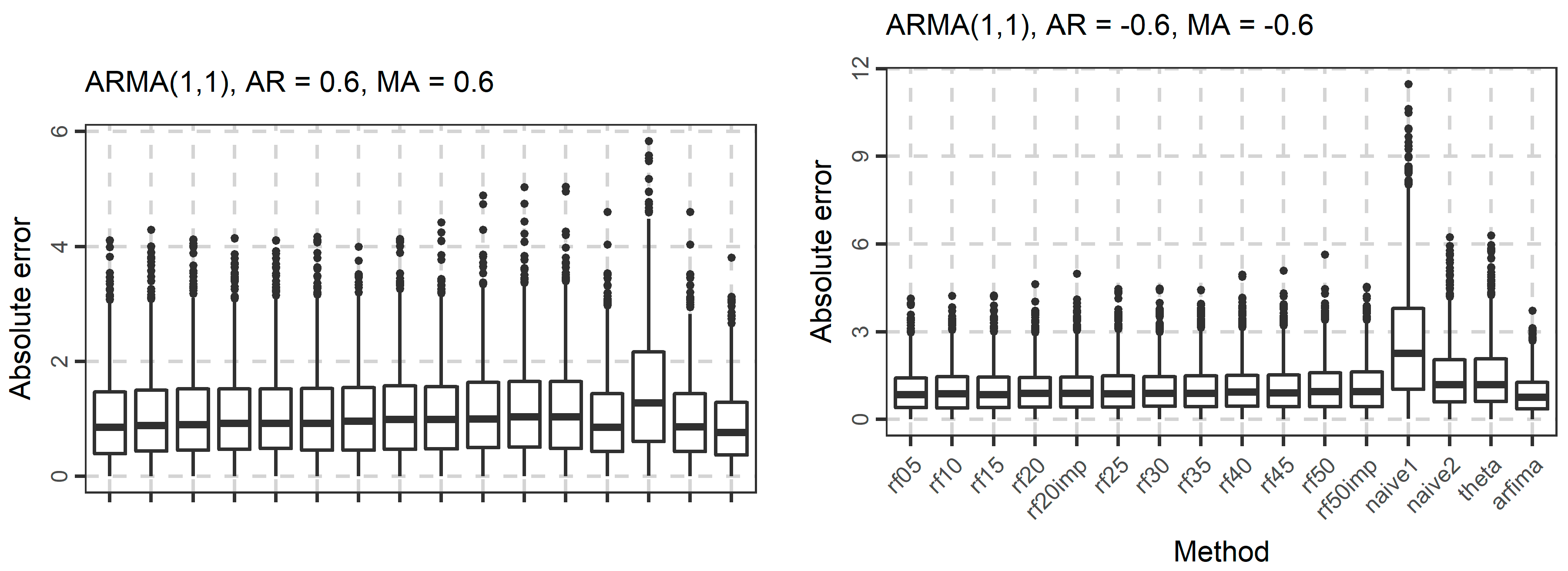
In Figure 4, Figure 5 and Figure 6, we present the boxplots of the absolute errors for the cases of the ARMA and ARFIMA models. It seems that in most cases, the rf methods with less predictor variables are better compared to the rf methods with many predictor variables according to the median of the absolute errors. The range of the absolute errors seems to get wider when using more predictor variables, as well as the number and the magnitude of outliers. The differences between all cases of the rf are small. The arfima method is the best, as expected, while the naïve and theta methods have varying predictive performance.
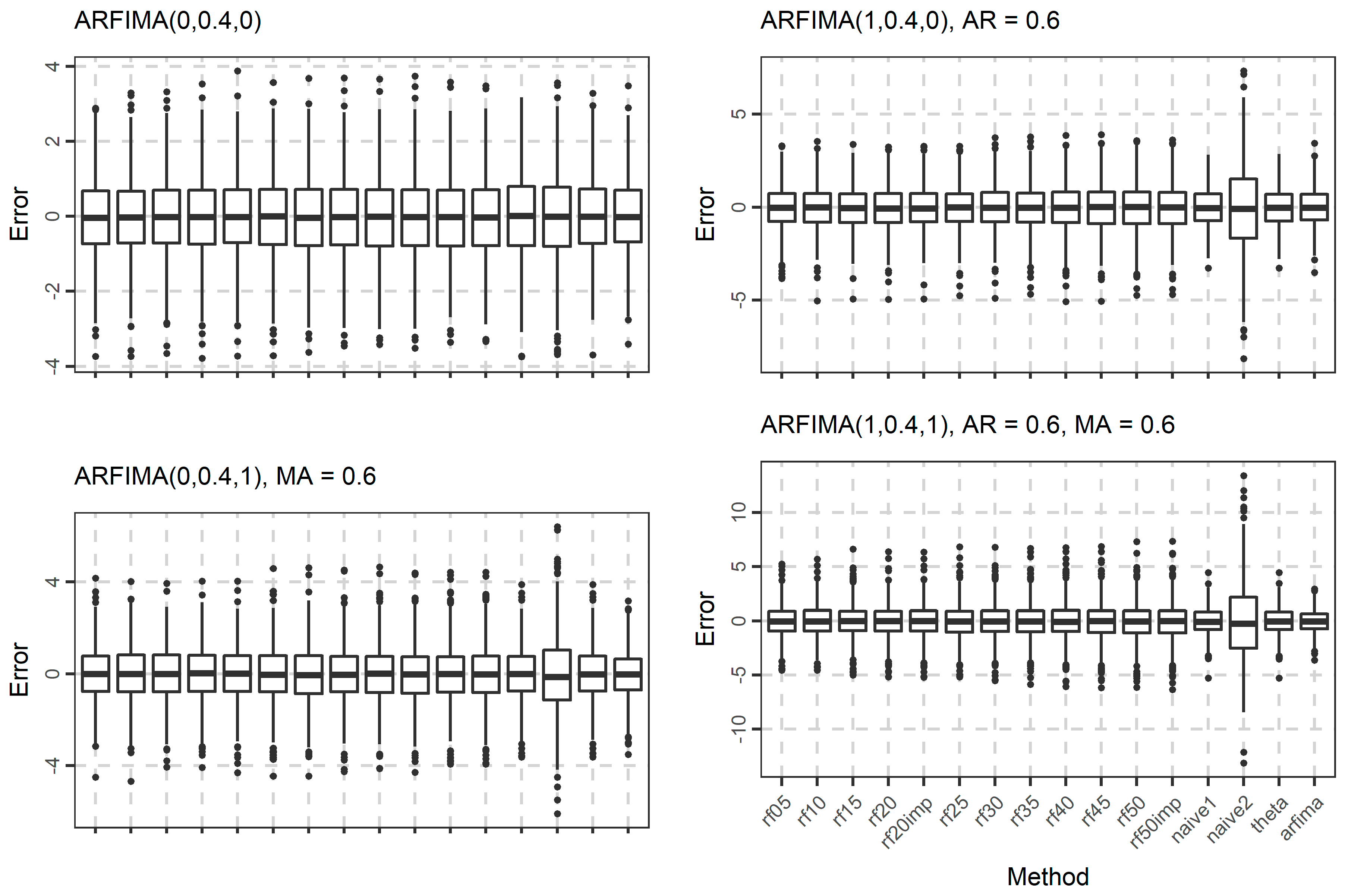
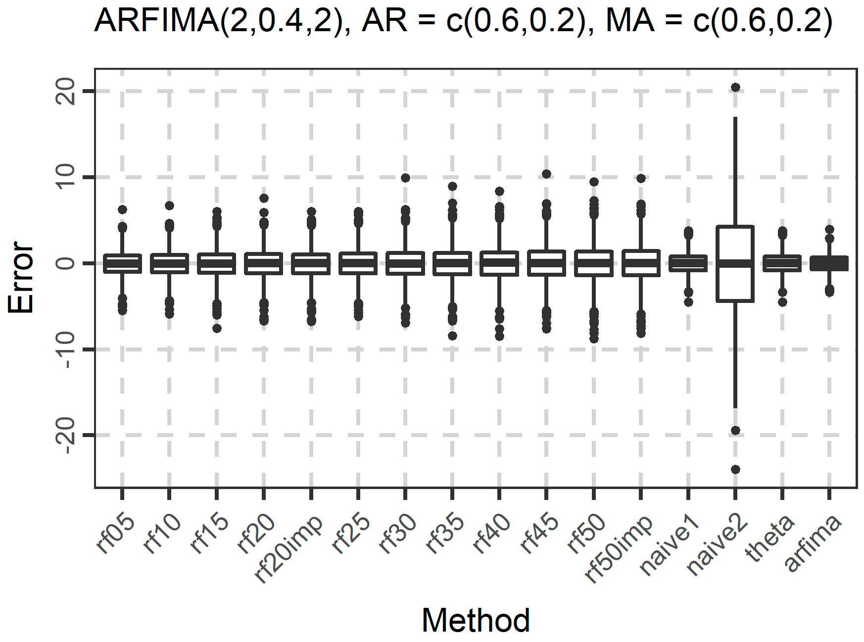
The distribution of the forecasts errors is also of interest. In Figure 7, Figure 8 and Figure 9, we present the boxplots of the errors for the ARMA and ARFIMA cases. All the methods are unbiased, in the sense that the median forecast error is approximately equal to 0, while most boxplots are symmetric around 0. The dispersion of the errors presented in Figure 7, Figure 8 and Figure 9 has already been quantified by the boxplots of the absolute errors in Figure 4, Figure 5 and Figure 6.
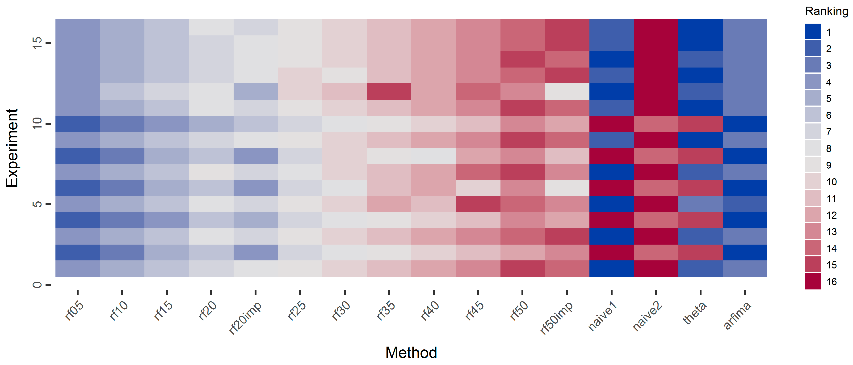
Given the vast amount of experiments and results, as well as the small differences between the performances of the various rf methods, we summarize the results using the rankings of the methods in each experiment, e.g., in Figure 10, we present the rankings of all methods in the simulation experiments with respect to the mean and median of the absolute errors. Due to the small differences between all the rf methods, a heatmap presenting the computed values for the mean and median of the absolute errors (and not their rankings) would be almost monochrome and, thus, not appropriate for the purpose of the present study.
Regarding the means of the absolute errors, the arfima method exhibits the best performance in all cases. In most cases of the ARMA simulation experiments (experiments numbered from one to 11), we observe that the rf methods are better than the rest methods. We observe a pattern in which the performance of the rf methods decreases when the number of predictor variables increases. The rf20imp method is generally better than the rf20 method, while the rf50imp method is worse than the rf50 method. The naïve and theta methods perform similarly. In the case of the ARFIMA simulations, the results are similar regarding the performance of the arfima methods and the intercomparison between the rf methods. However, in this case, the naïve1 and theta methods perform better than the rf methods.
When looking at the medians of the absolute errors, the arfima method has the best performance. In contrast to the cases of the means of the absolute errors, the pattern of the decreasing performance of the rf methods, when increasing the number of predictor variables is less uniform. Nevertheless, the overall pattern suggests that the performance of the rf decreases with the increase of the number of predictor variables. Importantly, Figure 10 highlights the competence of the rf methods in time series forecasting of small time series. In fact, rf exhibit better performance in comparison to all the methods but the arfima benchmark. This is definitely worth consideration.
Moreover, in Figure 11, we present the ranking of the methods with respect to the mean and median of the squared errors. The pattern is similar to that of Figure 10. Indeed the increase in the number of predictor variables decreases the performance of the RF algorithm.
In Figure 12, we present the ranking of the methods with respect to the regression coefficient. In general, the arfima methods are the best performing, while naïve2 is the worst method. We observe a pattern regarding the ARMA-simulated time series in which the naïve1 and theta methods are the best performing in the simulated experiments 1, 3, 5, 7, 9, and 11. In these experiments, the parameter values of the ARMA models are positive. In contrast, the simulation experiments 2, 4, 6, 8, and 10 correspond to ARMA models with at least one negative parameter.
Regarding the rf methods, they are almost uniformly better when using fewer predictor variables. Furthermore, the methods using important variables are better, compared to the respective methods, in which the full number of predictor variables is used.
3.2. Temperature Analysis
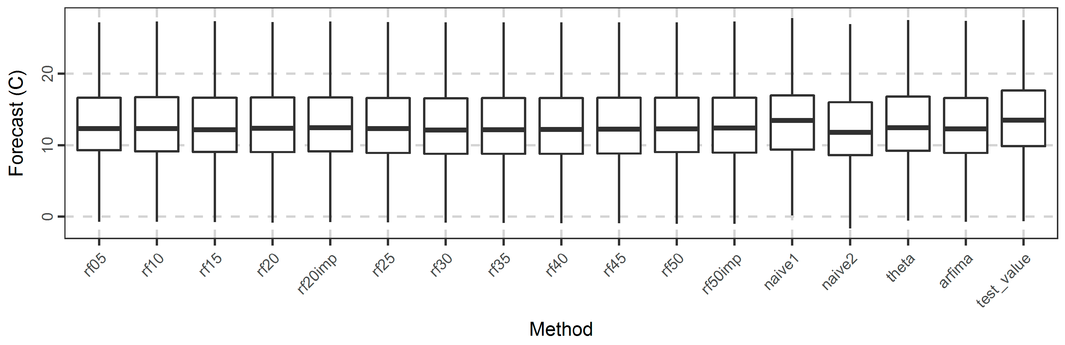
Regarding the application of the methods to the temperature dataset, we present the full results in the temperature_analysis.html file in Appendix A. Here we present some results necessary for the following discussion. In more detail, in Figure 13, we present the boxplots of the forecasts and their comparison to the test values. In terms of this specific comparison, naïve1 exhibits the best performance, since the median and range of its forecasts closely resemble the corresponding test values. The naïve2 method is the worst. The other methods are similar.
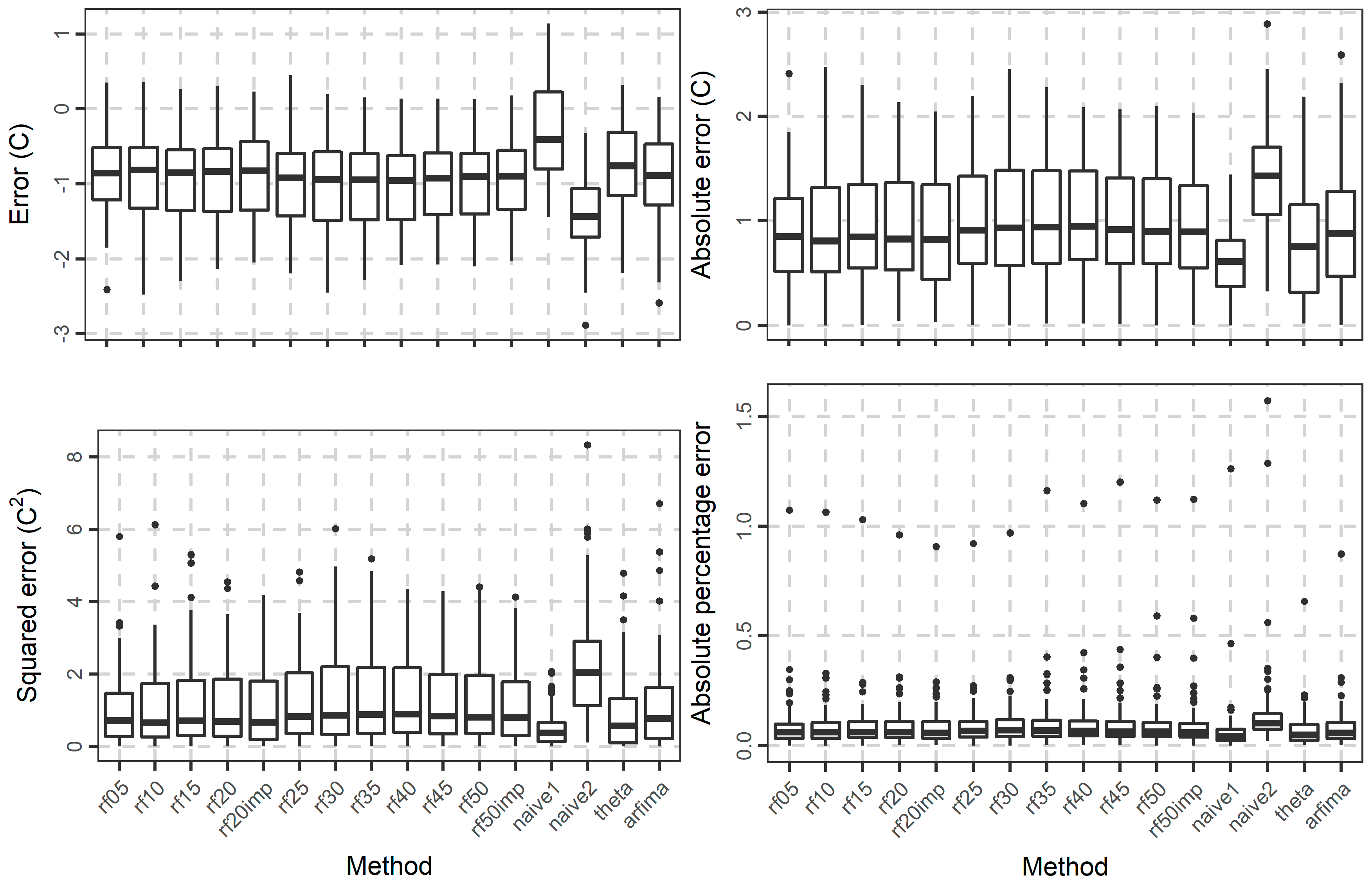
To highlight possible differences between the rf methods, we further present some comparisons based on the metric values. In Figure 14, we present the boxplots of the error, absolute error, squared error, and absolute percentage error values. The errors are mostly negative. Additionally, the respective distributions of the rf methods are closer to each other than to the respective distributions of naïve1, naïve2, and theta, while the distribution of the errors of the arfima method is rather closer to those of the rf methods. The same applies to the distributions of the other metrics. The far outliers produced in terms of absolute percentage error by almost all the methods can be explained by the presence of temperature values, which are close to zero.
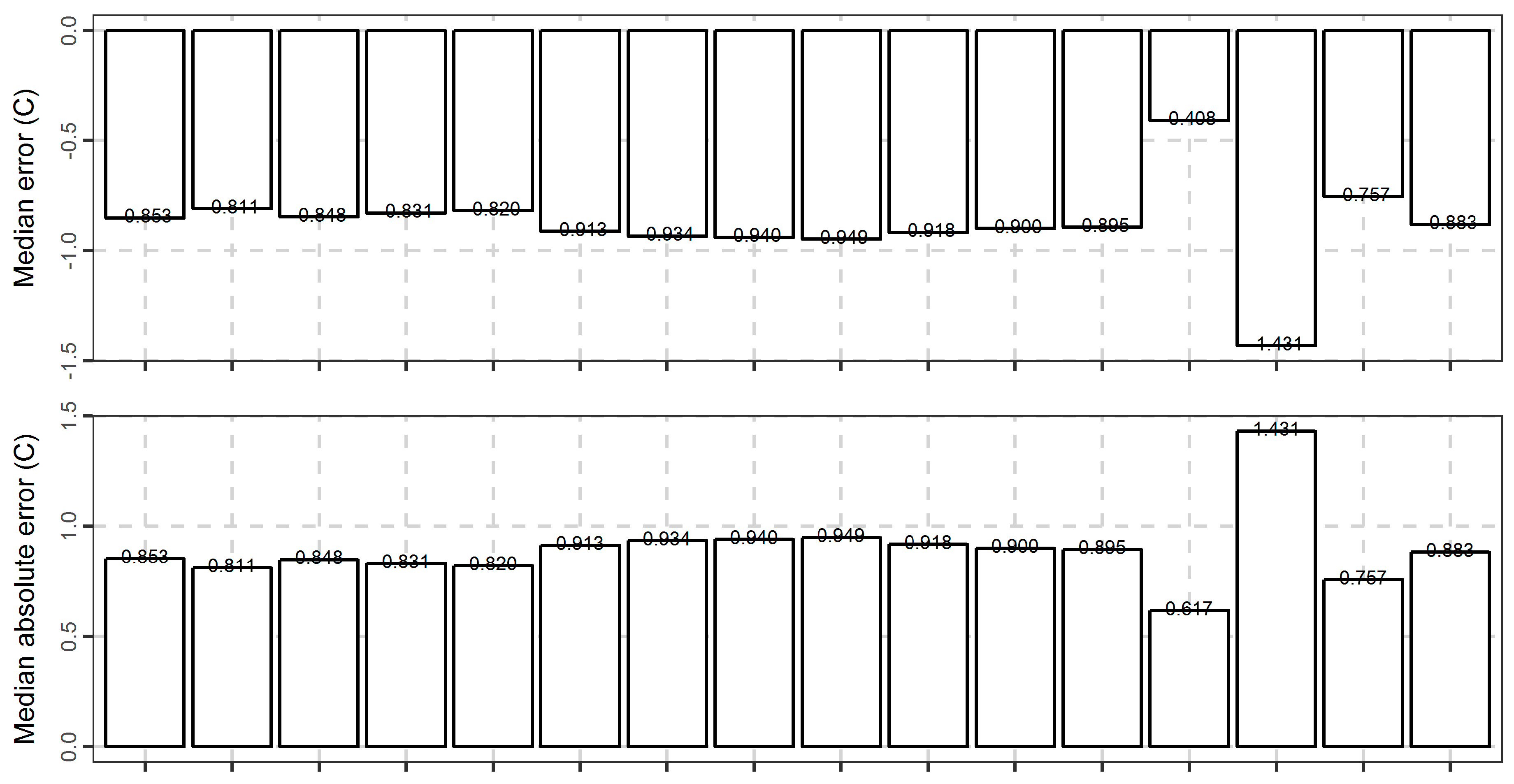
Moreover, Figure 15 focuses on the average-case performance of the methods with respect to all the computed metrics (presented in Section 2.1.9). A comparison with respect to this performance can ease the ranking of the methods. With regards to this particular ranking, the naïve1 and theta methods are clearly the best, while the naïve2 method is clearly the worst. The arfima method exhibits worse performance than naïve1 and theta, but better than the naïve2 method.
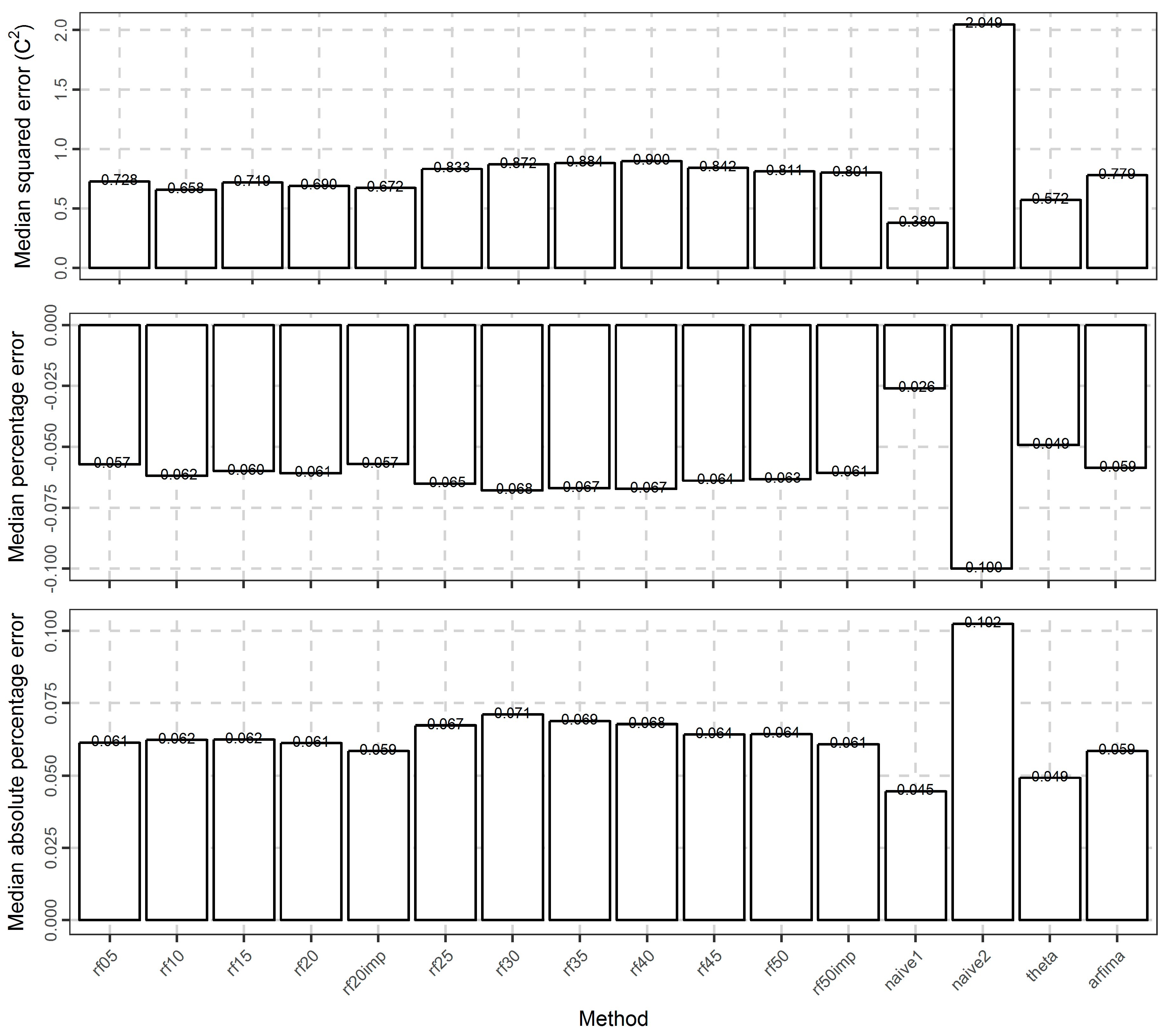
Regarding the rf methods, the best performance is exhibited by the rf10 method in terms of the median of errors, median of absolute error, and median of squared errors. On the contrary, with respect to the median of percentage errors and the median of absolute percentage errors the best rf method is rf20imp. In general, the performance of the rf05, rf10, rf15, rf20, rf20imp methods are close in terms of the median values of the metrics. The same applies to the performance of all the remaining rf methods, which nevertheless are worse. The arfima method has a similar performance with the worst rf methods.
In Figure 16, we present the regression coefficients between the forecasted and the test values. Here the differences between the methods are negligible. The best method is theta, followed by the rf05 and arfima methods. Moreover, the regression coefficient increases with the increase of the number of predictor variables. Additionally, using the important variables results in better results, e.g., rf20imp is better than rf20.
4. Discussion
Most of the studies focusing on time series forecasting aim at proposing a forecasting method based on its performance (compared to other methods, usually a few), when applied within a small number of case studies (e.g., [8,14,26,28,30]). Recognizing this specific fact and aiming at providing a tangible contribution in time series forecasting using RF, we have conducted an extensive set of computational experiments. These experiments were designed to create an empirical background on the effect of the variable selection on the forecasting performance, when implementing RF in one-step forecasting of short time series. We have examined two large datasets, a dataset composed of simulated time series and a temperature dataset. The latter is used complementary to the former for more concise findings.
The provided outcome is clear for the selected procedure of parameter tuning and for both the datasets examined and, thus, we would like to suggest its consideration in future applications. RF have performed better mostly when using a few recently lagged predictor variables. This outcome could be explained by the fact that increasing the number of lagged variables inevitably leads to reducing the length of the training set and concomitantly to reducing the information exploited from the original time series during the model fitting phase. On the contrary using many predictor variables in other types of regression problems does not seriously impact the predictive performance of RF [34] (p. 489).
In general, the results suggest that the RF algorithm performs well in one-step ahead forecasting of short time series. Nevertheless, other forecasting algorithms may exhibit better performance in some cases. This does not apply to every experiment conducted, neither does it imply that RF should not be used in one-step ahead time series forecasting in favour of these other algorithms as shown in [24,25,26,30]. In fact, in [12] the interested reader can find a small-scale comparison on 50 geophysical time series, which illustrates the fact that an algorithm can perform better or worse depending on the time series examined.
Furthermore, we focused on the RF algorithm and tried to improve its performance, under the condition that this algorithm was found to be competent. Therefore, there is a question of whether the condition that the random forests algorithm is competent is true, which will be answered in the following. The differences between the forecasting methods are mostly small and the performance of the RF algorithm is always comparable with the performance of other algorithms (this is the reason we used the ranking of the methods in the heatmaps and not the values of the metrics). The RF algorithm was found to be competent in the experiments using the simulated dataset, being worse than the arfima algorithm (a good benchmark for the case of the simulated time series) only, but in general better compared to the other methods (naïve1, naïve2, and theta methods). The RF algorithm was found to be competent in the experiment using the temperature dataset, being better than the arfima and naïve2 methods and worse than naïve1 and theta. We also found that the suboptimal RF (i.e., the ones that use many predictor variables) were mostly worse than the other methods, while the optimized RF were competent, thus highlighting the role of the variable selection in improving the performance of the RF.
Based on this fact, we would like to propose the use of a variety of algorithms in each forecasting application. Furthermore, since we believe that all the methodological choices (e.g., the variable selection in forecasting using machine learning) should be based on theory, or at least on evidence (which can be provided by extensive studies, like the present), rather than be made at will, we suggest that the performance of all the algorithms to be used in a specific application should have been previously optimized.
In addition to the main contribution of the present study, some other noteworthy findings have been derived through the analyses as well. These findings are summarized subsequently and highlight the merits of the adopted methodological framework. In general, we observe rather small differences between the various RF methods which, however, might be essential to some applications. Importantly, we observe that simple methods can perform extremely well with respect to the rest in specific autocorrelation schemes, as also concluded in other large comparisons (e.g., [37]) or reported by evidence in smaller studies (e.g., [12]). Particularly for the experiment conducted on real-world time series, we observe that the minimum absolute error in forecasting next year’s temperature using RF was approximately equal to 0.6 °C. This outcome is definitely important for geosciences, suggesting that temperature is a process difficult to forecast.
Moreover, the present study is one of the first applying benchmarking to assess the forecasting performance of random forests in time series forecasting and, therefore, a discussion about its effectiveness is meaningful. The achievement of a long-term optimal performance of a specific machine learning algorithm requires a firm strategy, which could result through studies like the present. Benchmarking was proven useful in highlighting the small magnitude of the differences between the various RF methods, while providing an upper and a lower bound in the performance of the latter, thus enabling one of the main conclusions, i.e., that RF is competent in one-step ahead forecasting of small time series. Therefore, we acknowledge the benefits of the benchmarking implementation within large-scale comparisons for creating a more faithful image of the goodness of performance characterizing the forecasting algorithms that can hardly be examined analytically, e.g., other machine learning algorithms.
Finally, reproducibility was a key consideration of this paper. The codes are available in the supplementary information, while the reader is encouraged to use them either for verification purposes, or for future research activities.
5. Conclusions
Random forests are amongst the most popular machine learning algorithms. The improvement of their performance in one-step forecasting of short time series was certainly worth attempting, since they have also proven to be a competent forecasting algorithm. These performance improvements and competencies are suggested by an extensive set of experiments, which use large datasets in conjunction with performance benchmarking. The results of these experiments clearly indicate that using a few recent variables as predictors during the fitting process leads to higher predictive accuracy for the random forest algorithm used in this study.
Of course, there are limitations in our study. In particular, the results were obtained using short time series, while there may be better procedures to find the optimal sets of parameters. However, this is the largest experiment conducted with the aforementioned aim. We hope that this outcome will be of use in future applications.
Supplementary Materials
The supplementary material is available online at www.mdpi.com/1999-4893/10/4/114/s1.
Acknowledgments
We thank three anonymous reviewers and the Academic Editor whose suggestions and comments helped in considerably improving the manuscript.
Author Contributions
The two authors worked on the paper and the implementation of the methodologies using the R programming language equally and on all of its aspects. However, Hristos Tyralis is the main writer of this paper and Georgia Papacharalampous conceived the idea.
Conflicts of Interest
The authors declare no conflict of interest.
Appendix A
The supplementary materials found as a zip file at http://dx.doi.org/10.17632/nr3z96jmbm.1 include all codes and data used in the manuscript. There is a readme file with detailed instructions on how to run each code and save the results. Two .html files, including the results and visualizations presented here, as well as more results which could not be included here for reasons of brevity, but enhance our finding,s can also be found in the supplementary material.
References
- Shmueli, G. To explain or to predict? Stat. Sci. 2010, 25, 289–310. [Google Scholar] [CrossRef]
- Bontempi, G.; Taieb, S.B.; Le Borgne, Y.A. Machine learning strategies for time series forecasting. In Business Intelligence (Lecture Notes in Business Information Processing); Aufaure, M.A., Zimányi, E., Eds.; Springer: Berlin/Heidelberg, Germany, 2013; Volume 138, pp. 62–77. [Google Scholar] [CrossRef]
- De Gooijer, J.G.; Hyndman, R.J. 25 years of time series forecasting. Int. J. Forecast. 2006, 22, 443–473. [Google Scholar] [CrossRef]
- Fildes, R.; Nikolopoulos, K.; Crone, S.F.; Syntetos, A.A. Forecasting and operational research: A review. J. Oper. Res. Soc. 2008, 59, 1150–1172. [Google Scholar] [CrossRef] [Green Version]
- Weron, R. Electricity price forecasting: A review of the state-of-the-art with a look into the future. Int. J. Forecast. 2014, 30, 1030–1081. [Google Scholar] [CrossRef]
- Hong, T.; Fan, S. Probabilistic electric load forecasting: A tutorial review. Int. J. Forecast. 2016, 32, 914–938. [Google Scholar] [CrossRef]
- Taieb, S.B.; Bontempi, G.; Atiya, A.F.; Sorjamaa, A. A review and comparison of strategies for multi-step ahead time series forecasting based on the NN5 forecasting competition. Expert Syst. Appl. 2012, 39, 7067–7083. [Google Scholar] [CrossRef]
- Mei-Ying, Y.; Xiao-Dong, W. Chaotic time series prediction using least squares support vector machines. Chin. Phys. 2004, 13, 454–458. [Google Scholar] [CrossRef]
- Faraway, J.; Chatfield, C. Time series forecasting with neural networks: A comparative study using the air line data. J. R. Stat. Soc. C Appl. Stat. 1998, 47, 231–250. [Google Scholar] [CrossRef]
- Yang, B.S.; Oh, M.S.; Tan, A.C.C. Machine condition prognosis based on regression trees and one-step-ahead prediction. Mech. Syst. Signal Process. 2008, 22, 1179–1193. [Google Scholar] [CrossRef]
- Zou, H.; Yang, Y. Combining time series models for forecasting. Int. J. Forecast. 2004, 20, 69–84. [Google Scholar] [CrossRef]
- Papacharalampous, G.A.; Tyralis, H.; Koutsoyiannis, D. Forecasting of geophysical processes using stochastic and machine learning algorithms. In Proceedings of the 10th World Congress of EWRA on Water Resources and Environment “Panta Rhei”, Athens, Greece, 5–9 July 2017. [Google Scholar]
- Pérez-Rodríguez, J.V.; Torra, S.; Andrada-Félix, J. STAR and ANN models: Forecasting performance on the Spanish “Ibex-35” stock index. J. Empir. Financ. 2005, 12, 490–509. [Google Scholar] [CrossRef]
- Khashei, M.; Bijari, M. A novel hybridization of artificial neural networks and ARIMA models for time series forecasting. Appl. Soft Comput. 2011, 11, 2664–2675. [Google Scholar] [CrossRef]
- Yan, W. Toward automatic time-series forecasting using neural networks. IEEE Trans. Neural Netw. Lear. Stat. 2012, 23, 1028–1039. [Google Scholar] [CrossRef]
- Babu, C.N.; Reddy, B.E. A moving-average filter based hybrid ARIMA–ANN model for forecasting time series data. Appl. Soft Comput. 2014, 23, 27–38. [Google Scholar] [CrossRef]
- Lin, L.; Wang, F.; Xie, X.; Zhong, S. Random forests-based extreme learning machine ensemble for multi-regime time series prediction. Expert Syst. Appl. 2017, 85, 164–176. [Google Scholar] [CrossRef]
- Breiman, L. Random Forests. Mach. Learn. 2001, 45, 5–32. [Google Scholar] [CrossRef]
- Scornet, E.; Biau, G.; Vert, J.P. Consistency of random forests. Ann. Stat. 2015, 43, 1716–1741. [Google Scholar] [CrossRef] [Green Version]
- Biau, G.; Scornet, E. A random forest guided tour. Test 2016, 25, 197–227. [Google Scholar] [CrossRef]
- Hastie, T.; Tibshirani, R.; Friedman, J. The Elements of Statistical Learning, 2nd ed.; Springer: New York, NY, USA, 2009. [Google Scholar] [CrossRef]
- Verikas, A.; Gelzinis, A.; Bacauskiene, M. Mining data with random forests: A survey and results of new tests. Pattern Recognit. 2011, 44, 330–349. [Google Scholar] [CrossRef]
- Herrera, M.; Torgo, L.; Izquierdo, J.; Pérez-García, R. Predictive models for forecasting hourly urban water demand. J. Hydrol. 2010, 387, 141–150. [Google Scholar] [CrossRef]
- Dudek, G. Short-term load forecasting using random forests. In Proceedings of the 7th IEEE International Conference Intelligent Systems IS’2014 (Advances in Intelligent Systems and Computing), Warsaw, Poland, 24–26 September 2014; Filev, D., Jabłkowski, J., Kacprzyk, J., Krawczak, M., Popchev, I., Rutkowski, L., Sgurev, V., Sotirova, E., Szynkarczyk, P., Zadrozny, S., Eds.; Springer: Cham, Switzerland, 2015; Volume 323, pp. 821–828. [Google Scholar] [CrossRef]
- Chen, J.; Li, M.; Wang, W. Statistical uncertainty estimation using random forests and its application to drought forecast. Math. Probl. Eng. 2012, 2012, 915053. [Google Scholar] [CrossRef]
- Naing, W.Y.N.; Htike, Z.Z. Forecasting of monthly temperature variations using random forests. APRN J. Eng. Appl. Sci. 2015, 10, 10109–10112. [Google Scholar]
- Nguyen, T.T.; Huu, Q.N.; Li, M.J. Forecasting time series water levels on Mekong river using machine learning models. In Proceedings of the 2015 Seventh International Conference on Knowledge and Systems Engineering (KSE), Ho Chi Minh City, Vietnam, 8–10 October 2015. [Google Scholar] [CrossRef]
- Kumar, M.; Thenmozhi, M. Forecasting stock index movement: A comparison of support vector machines and random forest. In Indian Institute of Capital Markets 9th Capital Markets Conference Paper; Indian Institute of Capital Markets: Vashi, India, 2006. [Google Scholar] [CrossRef]
- Kumar, M.; Thenmozhi, M. Forecasting stock index returns using ARIMA-SVM, ARIMA-ANN, and ARIMA-random forest hybrid models. Int. J. Bank. Acc. Financ. 2014, 5, 284–308. [Google Scholar] [CrossRef]
- Kane, M.J.; Price, N.; Scotch, M.; Rabinowitz, P. Comparison of ARIMA and Random Forest time series models for prediction of avian influenza H5N1 outbreaks. BMC Bioinform. 2014, 15. [Google Scholar] [CrossRef] [PubMed]
- Genuer, R.; Poggi, J.M.; Tuleau-Malot, C. Variable selection using random forests. Pattern Recognit. Lett. 2010, 31, 2225–2236. [Google Scholar] [CrossRef]
- Oshiro, T.M.; Perez, P.S.; Baranauskas, J.A. How many trees in a random forest? In Machine Learning and Data Mining in Pattern Recognition (Lecture Notes in Computer Science); Perner, P., Ed.; Springer: Berlin/Heidelberg, Germany, 2012; pp. 154–168. [Google Scholar] [CrossRef]
- Probst, P.; Boulesteix, A.L. To tune or not to tune the number of trees in random forest? arXiv 2017, arXiv:1705.05654v1. [Google Scholar]
- Kuhn, M.; Johnson, K. Applied Predictive Modeling; Springer: New York, NY, USA, 2013. [Google Scholar] [CrossRef]
- Díaz-Uriarte, R.; De Andres, S.A. Gene selection and classification of microarray data using random forest. BMC Bioinform. 2006, 7. [Google Scholar] [CrossRef] [PubMed]
- Makridakis, S.; Hibon, M. Confidence intervals: An empirical investigation of the series in the M-competition. Int. J. Forecast. 1987, 3, 489–508. [Google Scholar] [CrossRef]
- Makridakis, S.; Hibon, M. The M3-Competition: Results, conclusions and implications. Int. J. Forecast. 2000, 16, 451–476. [Google Scholar] [CrossRef]
- Pritzsche, U. Benchmarking of classical and machine-learning algorithms (with special emphasis on bagging and boosting approaches) for time series forecasting. Master’s Thesis, Ludwig-Maximilians-Universität München, München, Germany, 2015. [Google Scholar]
- Bagnall, A.; Cawley, G.C. On the use of default parameter settings in the empirical evaluation of classification algorithms. arXiv 2017, arXiv:1703.06777v1. [Google Scholar]
- Salles, R.; Assis, L.; Guedes, G.; Bezerra, E.; Porto, F.; Ogasawara, E. A framework for benchmarking machine learning methods using linear models for univariate time series prediction. In Proceedings of the 2017 International Joint Conference on Neural Networks (IJCNN), Anchorage, AK, USA, 14–19 May 2017; pp. 2338–2345. [Google Scholar] [CrossRef]
- Bontempi, G. Machine Learning Strategies for Time Series Prediction. European Business Intelligence Summer School, Hammamet, Lecture. 2013. Available online: https://pdfs.semanticscholar.org/f8ad/a97c142b0a2b1bfe20d8317ef58527ee329a.pdf (accessed on 25 September 2017).
- McShane, B.B. Machine Learning Methods with Time Series Dependence. Ph.D. Thesis, University of Pennsylvania, Philadelphia, PA, USA, 2010. [Google Scholar]
- Bagnall, A.; Bostrom, A.; Large, J.; Lines, J. Simulated data experiments for time series classification part 1: Accuracy comparison with default settings. arXiv 2017, arXiv:1703.09480v1. [Google Scholar]
- Box, G.E.P.; Jenkins, G.M. Some recent advances in forecasting and control. J. R. Stat. Soc. C Appl. Stat. 1968, 17, 91–109. [Google Scholar] [CrossRef]
- Wei, W.W.S. Time Series Analysis, Univariate and Multivariate Methods, 2nd ed.; Pearson Addison Wesley: Boston, MA, USA, 2006; ISBN 0-321-322116-9. [Google Scholar]
- Thissen, U.; Van Brakel, R.; De Weijer, A.P.; Melssena, W.J.; Buydens, L.M.C. Using support vector machines for time series prediction. Chemom. Intell. Lab. 2003, 69, 35–49. [Google Scholar] [CrossRef]
- Zhang, G.P. An investigation of neural networks for linear time-series forecasting. Comput. Oper. Res. 2001, 28, 1183–1202. [Google Scholar] [CrossRef]
- Lawrimore, J.H.; Menne, M.J.; Gleason, B.E.; Williams, C.N.; Wuertz, D.B.; Vose, R.S.; Rennie, J. An overview of the Global Historical Climatology Network monthly mean temperature data set, version 3. J. Geophys. Res. 2011, 116. [Google Scholar] [CrossRef]
- Assimakopoulos, V.; Nikolopoulos, K. The theta model: A decomposition approach to forecasting. Int. J. Forecast. 2000, 16, 521–530. [Google Scholar] [CrossRef]
- Kuhn, M. Building predictive models in R using the caret package. J. Stat. Softw. 2008, 28. [Google Scholar] [CrossRef]
- Kuhn, M.; Wing, J.; Weston, S.; Williams, A.; Keefer, C.; Engelhardt, A.; Cooper, T.; Mayer, Z.; Kenkel, B.; The R Core Team; et al. Caret: Classification and Regression Training, R package version 6.0-76; 2017. Available online: https://cran.r-project.org/web/packages/caret/index.html (accessed on 7 September 2017).
- The R Core Team. R: A Language and Environment for Statistical Computing; R Foundation for Statistical Computing: Vienna, Austria, 2017. [Google Scholar]
- Hemelrijk, J. Underlining random variables. Stat. Neerl. 1966, 20, 1–7. [Google Scholar] [CrossRef]
- Fraley, C.; Leisch, F.; Maechler, M.; Reisen, V.; Lemonte, A. Fracdiff: Fractionally Differenced ARIMA aka ARFIMA(p,d,q) Models, R package version 1.4-2. 2012. Available online: https://rdrr.io/cran/fracdiff/(accessed on 2 December 2012).
- Hyndman, R.J.; O’Hara-Wild, M.; Bergmeir, C.; Razbash, S.; Wang, E. Forecast: Forecasting Functions for Time Series and Linear Models, R package version 8.1. 2017. Available online: https://rdrr.io/cran/forecast/(accessed on 25 September 2017).
- Hyndman, R.J.; Khandakar, Y. Automatic time series forecasting: The forecast package for R. J. Stat. Softw. 2008, 27. [Google Scholar] [CrossRef]
- Hyndman, R.J.; Athanasopoulos, G. Forecasting: Principles and Practice; OTexts: Melbourne, Australia, 2013. Available online: http://otexts.org/fpp/ (accessed on 25 September 2017).
- Hyndman, R.J.; Billah, B. Unmasking the Theta method. Int. J. Forecast. 2003, 19, 287–290. [Google Scholar] [CrossRef]
- Hyndman, R.J.; Koehler, A.B.; Ord, J.K.; Snyder, R.D. Forecasting with Exponential Smoothing: The State Space Approach; Springer: Berlin/Heidelberg, Germany, 2008. [Google Scholar] [CrossRef]
- Liaw, A.; Wiener, M. Classification and Regression by randomForest. R News 2002, 2, 18–22. [Google Scholar]
- Cortez, P. Data mining with neural networks and support vector machines using the R/rminer tool. In Advances in Data Mining. Applications and Theoretical Aspects (Lecture Notes in Artificial Intelligence); Perner, P., Ed.; Springer: Berlin/Heidelberg, Germany, 2010; Volume 6171, pp. 572–583. [Google Scholar] [CrossRef] [Green Version]
- Cortez, P. Rminer: Data Mining Classification and Regression Methods, R package version 1.4.2. 2016. Available online: https://rdrr.io/cran/rminer/(accessed on 2 September 2016).
- Hyndman, R.J.; Koehler, A.B. Another look at measures of forecast accuracy. Int. J. Forecast. 2006, 22, 679–688. [Google Scholar] [CrossRef]
- Alexander, D.L.J.; Tropsha, A.; Winkler, D.A. Beware of R2: Simple, unambiguous assessment of the prediction accuracy of QSAR and QSPR models. J. Chem. Inf. Model. 2015, 55, 1316–1322. [Google Scholar] [CrossRef] [PubMed]
- Gramatica, P.; Sangion, A. A historical excursus on the statistical validation parameters for QSAR models: A clarification concerning metrics and terminology. J. Chem. Inf. Model. 2016, 56, 1127–1131. [Google Scholar] [CrossRef] [PubMed]
- Warnes, G.R.; Bolker, B.; Gorjanc, G.; Grothendieck, G.; Korosec, A.; Lumley, T.; MacQueen, D.; Magnusson, A.; Rogers, J. Gdata: Various R Programming Tools for Data Manipulation, R package version 2.18.0. 2017. Available online: https://cran.r-project.org/web/packages/gdata/index.html(accessed on 6 June 2017).
- Wickham, H. Ggplot2: Elegant Graphics for Data Analysis, 2nd ed.; Springer International Publishing: Cham, Switzerland, 2016. [Google Scholar] [CrossRef]
- Wickham, H.; Hester, J.; Francois, R.; Jylänki, J.; Jørgensen, M. Readr: Read Rectangular Text Data, R package version 1.1.1; 2017; Available online: https://cran.r-project.org/web/packages/readr/index.html (accessed on 16 May 2017).
- Wickham, H. Reshaping data with the reshape package. J. Stat. Softw. 2007, 21. [Google Scholar] [CrossRef]
Figure 1.
Sketch explaining how the training sample changes with the number of predictor variables for time series with n = 5 and (a) k = 1; (b) k = 2.
Figure 1.
Sketch explaining how the training sample changes with the number of predictor variables for time series with n = 5 and (a) k = 1; (b) k = 2.

Figure 2.
Map of locations for the 135 stations used in the analysis.

Figure 3.
Barplots of the medians of the absolute errors, medians of the squared errors and regression coefficients when forecasting the 101st value of 1000 simulated time series from an ARMA(1, 0) model with φ1 = 0.6.
Figure 3.
Barplots of the medians of the absolute errors, medians of the squared errors and regression coefficients when forecasting the 101st value of 1000 simulated time series from an ARMA(1, 0) model with φ1 = 0.6.
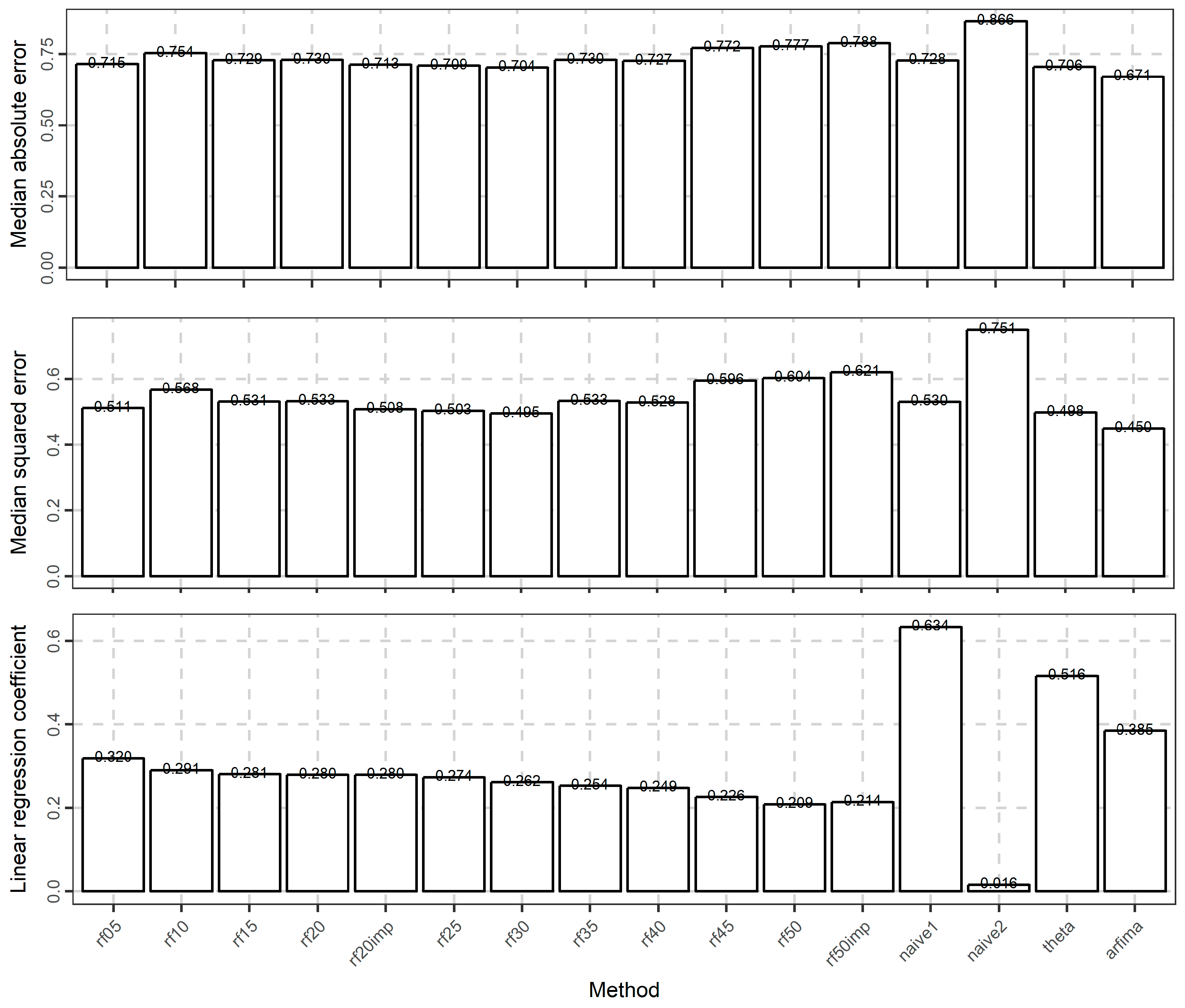
Figure 4.
Boxplots of the absolute errors when forecasting the 101st value of 1000 simulated time series from each ARMA(p, 0) and ARMA(0, q) model used in the present study.
Figure 4.
Boxplots of the absolute errors when forecasting the 101st value of 1000 simulated time series from each ARMA(p, 0) and ARMA(0, q) model used in the present study.

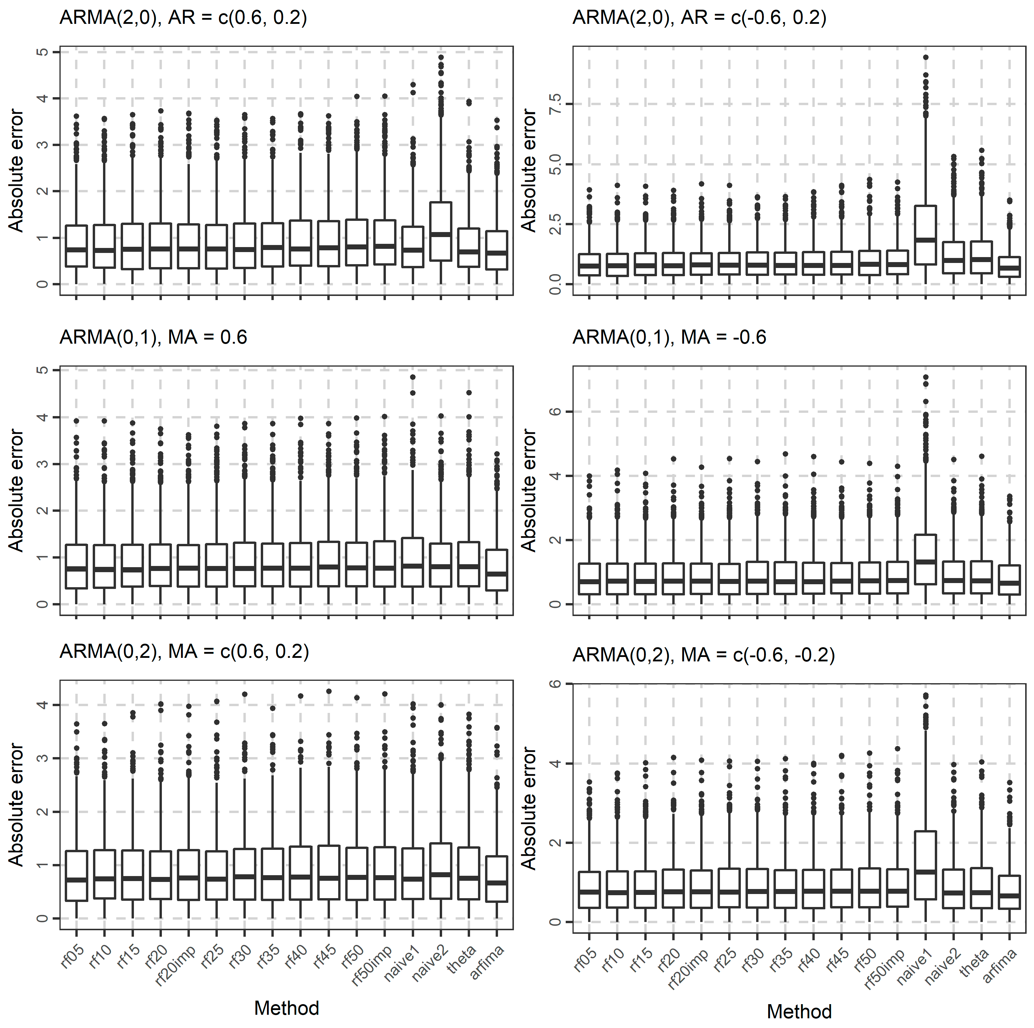
Figure 5.
Boxplots of the absolute errors when forecasting the 101st value of 1000 simulated time series from each ARMA(p, q) model used in the present study.
Figure 5.
Boxplots of the absolute errors when forecasting the 101st value of 1000 simulated time series from each ARMA(p, q) model used in the present study.

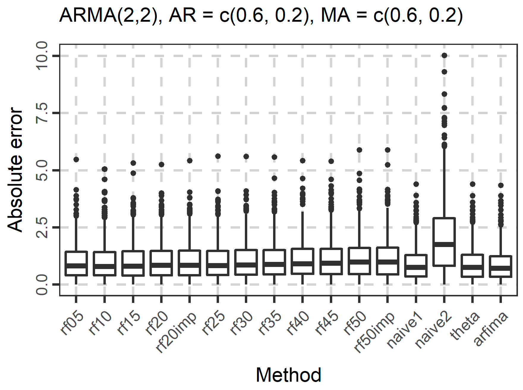
Figure 6.
Boxplots of the absolute errors when forecasting the 101st value of 1000 simulated time series from each ARFIMA model used in the present study.
Figure 6.
Boxplots of the absolute errors when forecasting the 101st value of 1000 simulated time series from each ARFIMA model used in the present study.
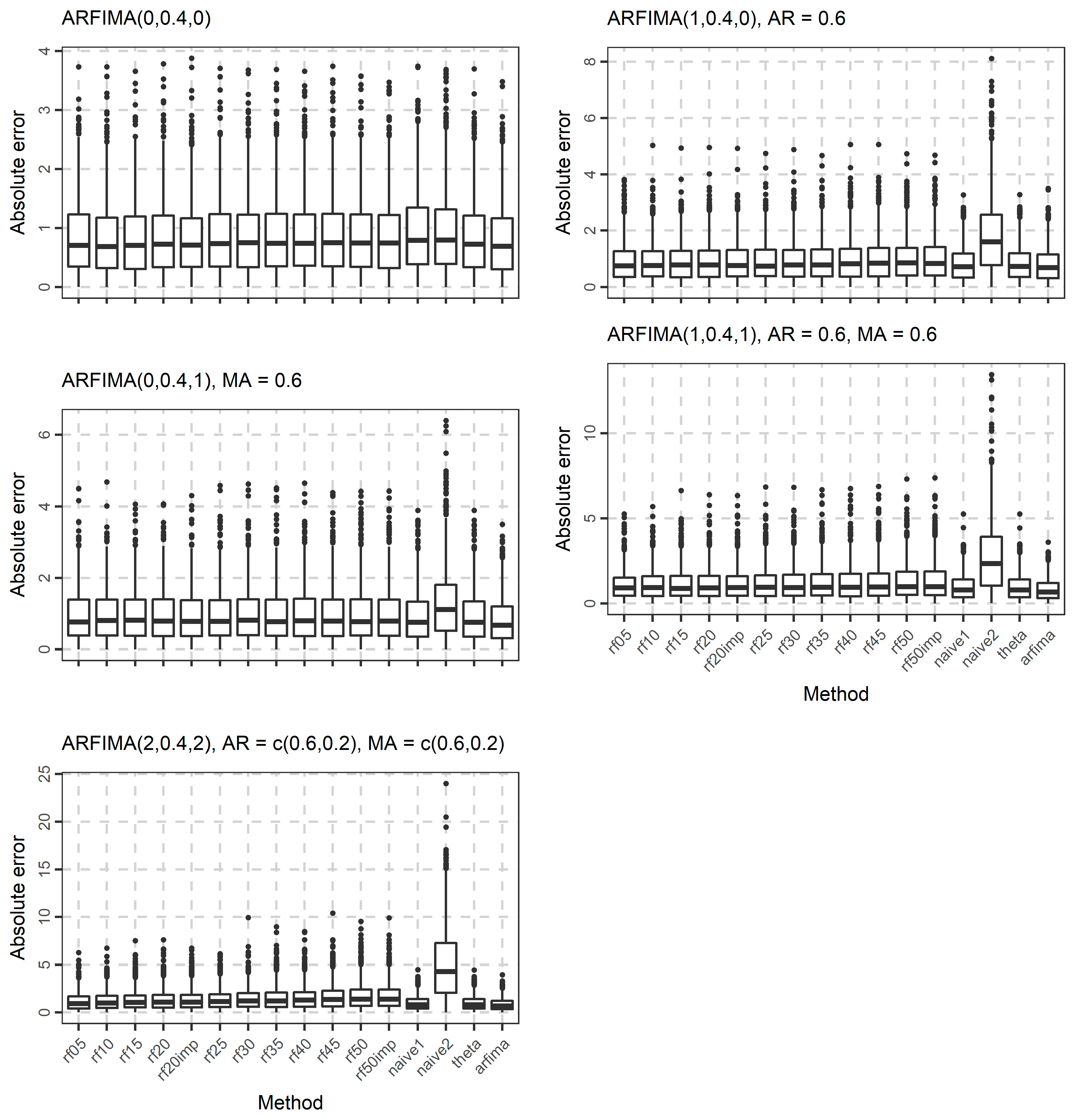
Figure 7.
Boxplots of the errors when forecasting the 101st value of 1000 simulated time series from each ARMA(p, 0) and ARMA(0, q) model used in the present study.
Figure 7.
Boxplots of the errors when forecasting the 101st value of 1000 simulated time series from each ARMA(p, 0) and ARMA(0, q) model used in the present study.
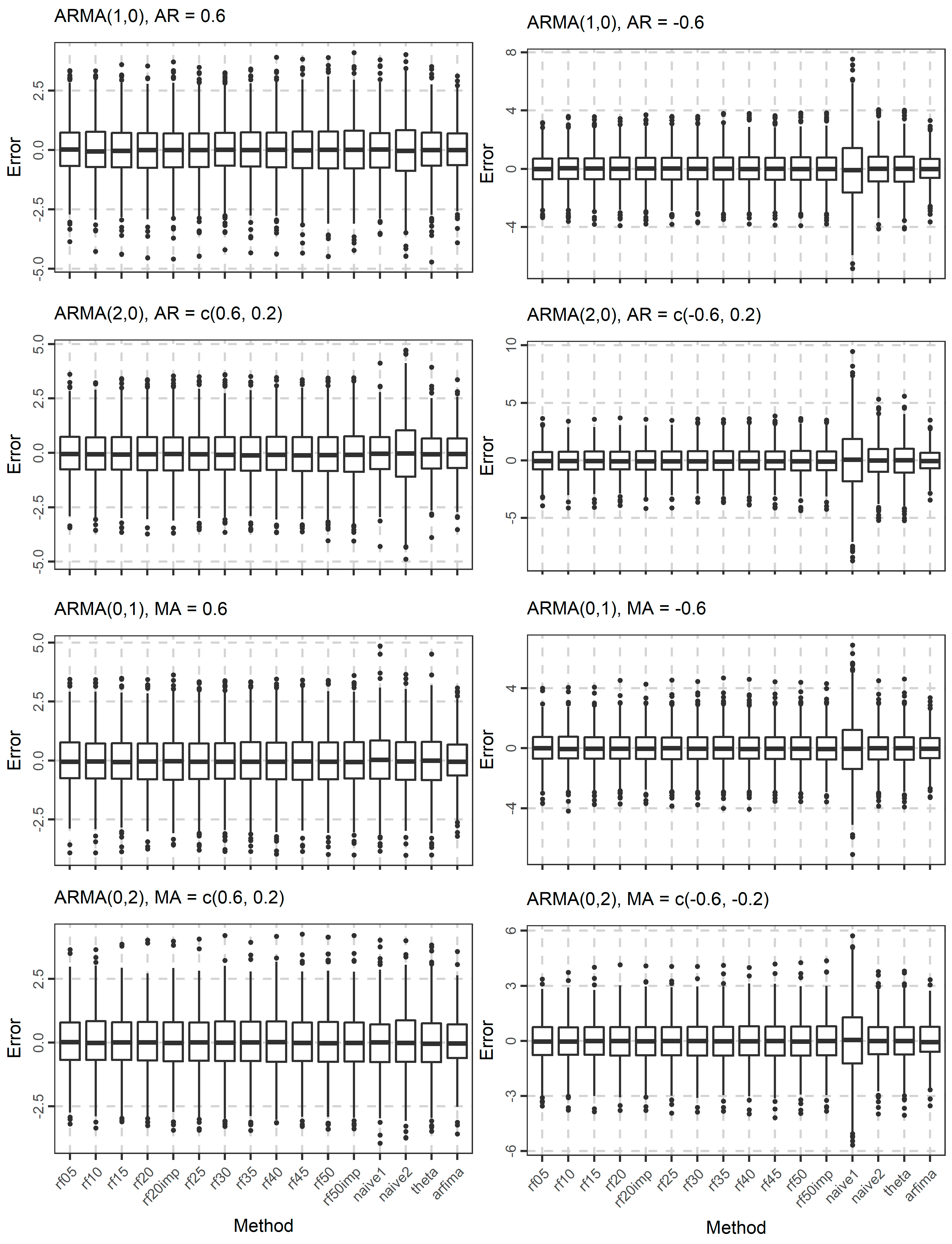
Figure 8.
Boxplots of the errors when forecasting the 101st value of 1000 simulated time series from each ARMA(p, q) model used in the present study.
Figure 8.
Boxplots of the errors when forecasting the 101st value of 1000 simulated time series from each ARMA(p, q) model used in the present study.
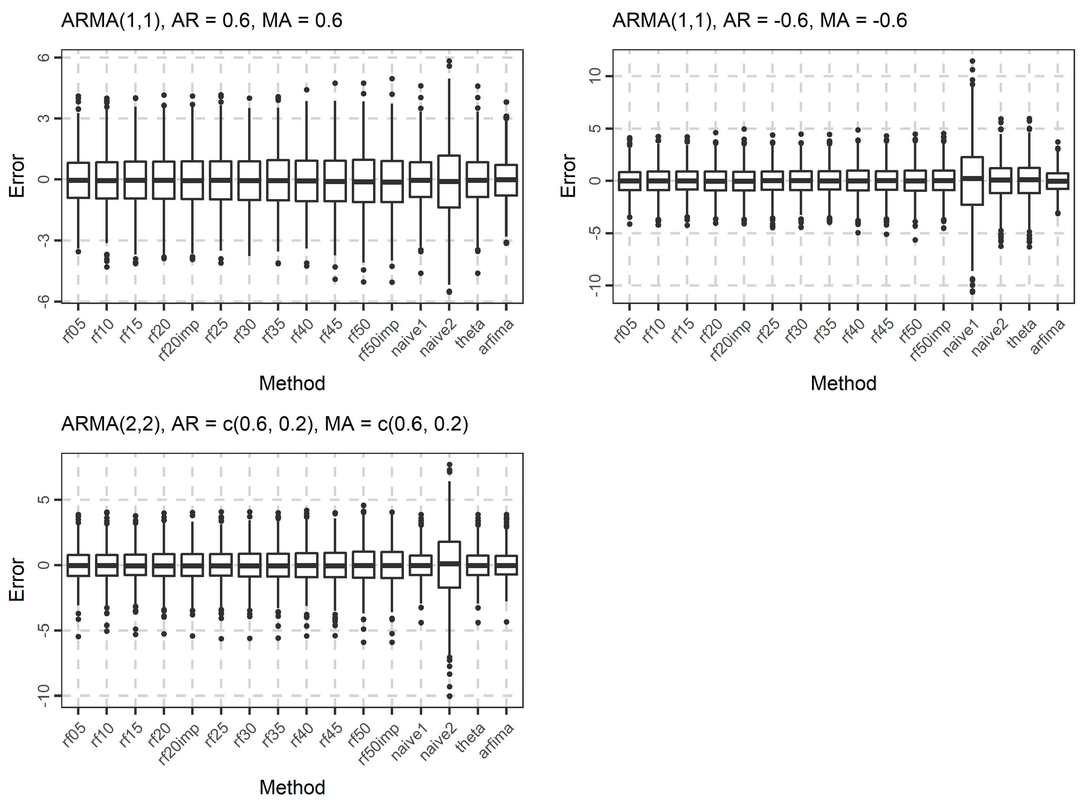
Figure 9.
Boxplots of the errors when forecasting the 101st value of 1000 simulated time series from each ARFIMA model used in the present study.
Figure 9.
Boxplots of the errors when forecasting the 101st value of 1000 simulated time series from each ARFIMA model used in the present study.


Figure 10.
Ranking of methods within each simulation experiment based on the mean (top) and median (bottom) of the absolute errors. Better methods are presented with lower ranking value and blue colours.
Figure 10.
Ranking of methods within each simulation experiment based on the mean (top) and median (bottom) of the absolute errors. Better methods are presented with lower ranking value and blue colours.
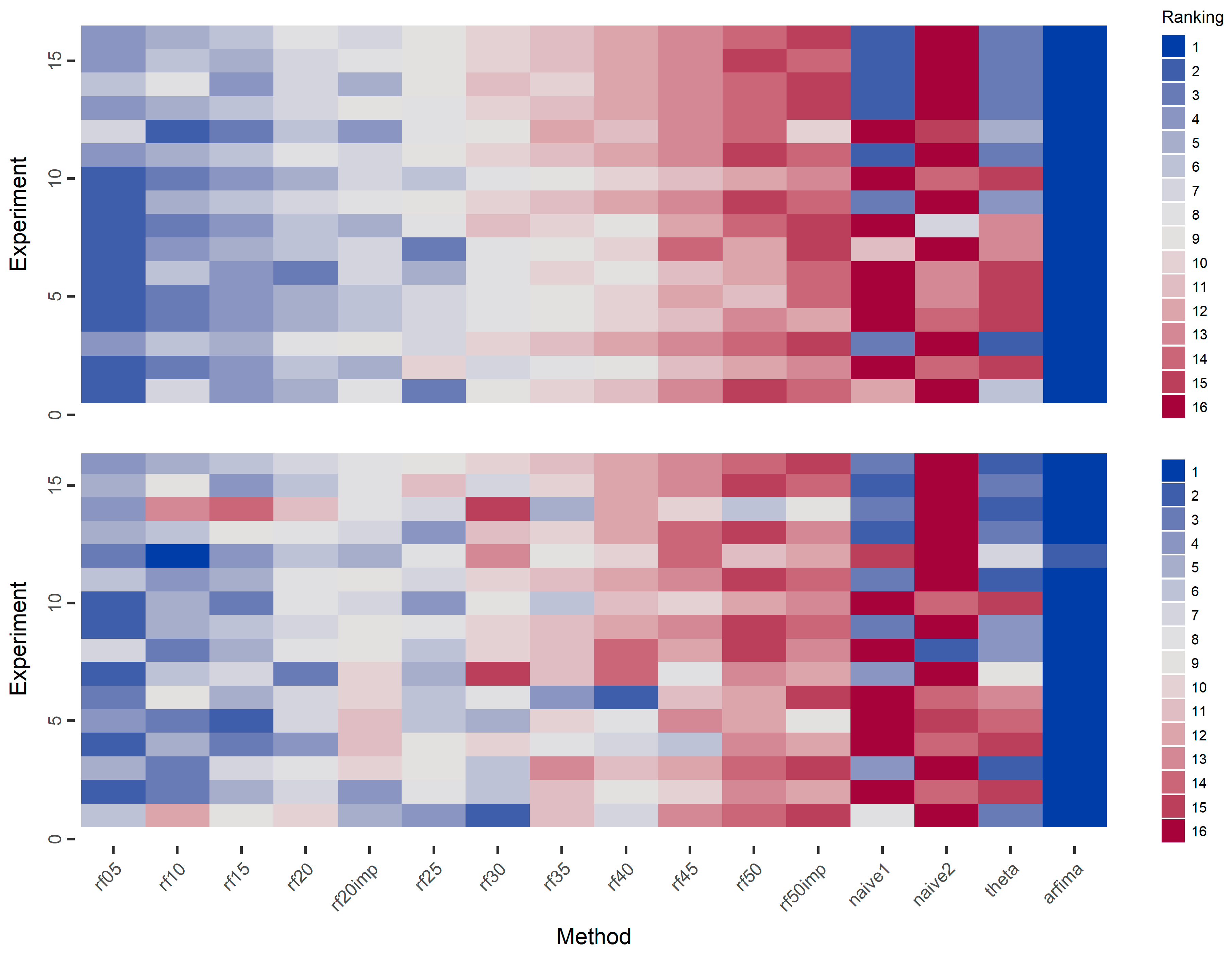
Figure 11.
Ranking of methods in each simulation experiment based on the mean (top) and median (bottom) of the squared errors. Better methods are presented with lower ranking value and blue colours.
Figure 11.
Ranking of methods in each simulation experiment based on the mean (top) and median (bottom) of the squared errors. Better methods are presented with lower ranking value and blue colours.
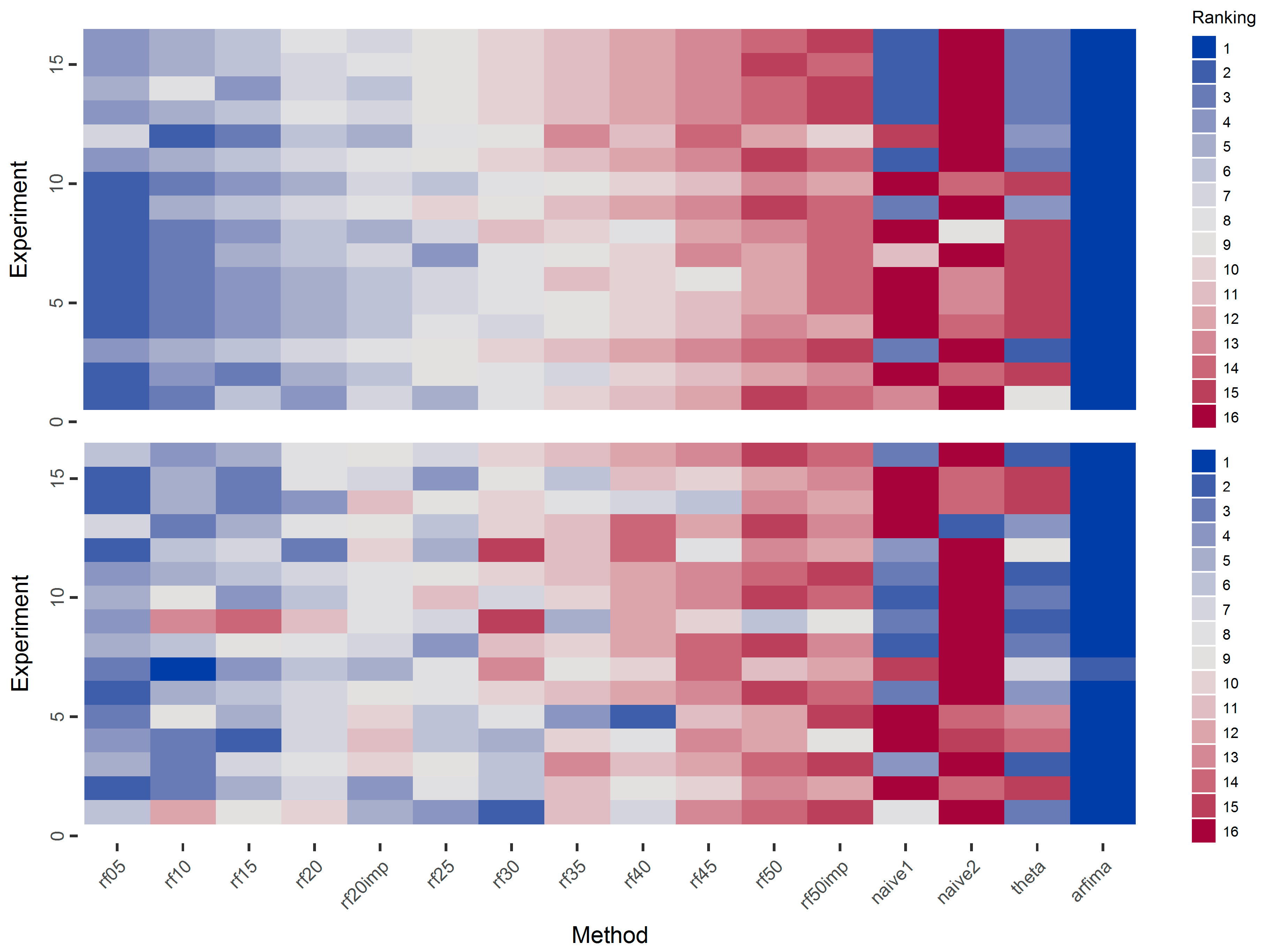
Figure 12.
Ranking of methods in each simulation experiment based on the regression coefficients. Better methods are presented with lower ranking value and blue colours.
Figure 12.
Ranking of methods in each simulation experiment based on the regression coefficients. Better methods are presented with lower ranking value and blue colours.

Figure 13.
Boxplot of forecasts of temperature for each method.

Figure 14.
Boxplots of the error, absolute error, squared error, and absolute percentage error values of the temperature forecasts for all the methods.
Figure 14.
Boxplots of the error, absolute error, squared error, and absolute percentage error values of the temperature forecasts for all the methods.

Figure 15.
Barplots of the medians of various types of metrics measuring the error of the temperature forecasts for all the methods. The types of errors are depicted in the vertical axes.
Figure 15.
Barplots of the medians of various types of metrics measuring the error of the temperature forecasts for all the methods. The types of errors are depicted in the vertical axes.


Figure 16.
Barplots of the regression coefficient of the linear model between the forecasted and the test values of the temperature dataset.
Figure 16.
Barplots of the regression coefficient of the linear model between the forecasted and the test values of the temperature dataset.

Table 1.
Summary of the methods presented in Section 2.1.3, Section 2.1.4, Section 2.1.5, Section 2.1.6 and Section 2.1.7 and their abbreviation as used in Section 3.
Table 1.
Summary of the methods presented in Section 2.1.3, Section 2.1.4, Section 2.1.5, Section 2.1.6 and Section 2.1.7 and their abbreviation as used in Section 3.
| Method | Section | Brief Explanation |
|---|---|---|
| arfima | 2.1.3 | Uses fitted ARMA or ARFIMA models |
| naïve1 | 2.1.4 | Forecast equal to the last observed value, Equation (16) |
| naïve2 | 2.1.4 | Forecast equal to the mean of the fitted set, Equation (17) |
| theta | 2.1.5 | Uses the theta method |
| rf | 2.1.7 | Uses random forests, Equation (20) |
Table 2.
Methods presented in Section 2.1.3 for forecasting using ARMA and ARFIMA models and their specific applications in Section 3.
Table 2.
Methods presented in Section 2.1.3 for forecasting using ARMA and ARFIMA models and their specific applications in Section 3.
| Method | Application in Section 3 |
|---|---|
| 1st case in Section 2.1.3 | Simulations from the family of ARMA models |
| 2nd case in Section 2.1.3 | Simulations from the family of ARFIMA models, with d ≠ 0 |
| 2nd case in Section 2.1.3 | Temperature data |
Table 3.
Variable selection procedures used by the RF algorithm.
| Method | Explanatory Variables |
|---|---|
| rf05, rf10, rf15, rf20, rf25, rf30, rf35, rf40, rf45, rf50 | Uses the last 5, …, 50 variables |
| rf20imp, rf50imp | Uses the most important variables from the last 20 and 50 variables respectively |
Table 4.
Metrics of forecasting performance, their range and respective values when the forecast is perfect.
Table 4.
Metrics of forecasting performance, their range and respective values when the forecast is perfect.
| Metric | Equation | Range | Metric Values for Perfect Forecast |
|---|---|---|---|
| error | (21) | [−∞, ∞] | 0 |
| absolute error | (22) | [0, ∞] | 0 |
| squared error | (23) | [0, ∞] | 0 |
| percentage error | (24) | [−∞, ∞] | 0 |
| absolute percentage error | (25) | [0, ∞] | 0 |
| linear regression coefficient | (36) | [−∞, ∞] | 1 |
Table 5.
Simulation experiments, their respective models and their defined parameters. See Section 2.1.1 for the definitions of the parameters.
Table 5.
Simulation experiments, their respective models and their defined parameters. See Section 2.1.1 for the definitions of the parameters.
| Experiment | Model | Parameters |
|---|---|---|
| 1 | ARMA(1, 0) | φ1 = 0.6 |
| 2 | ARMA(1, 0) | φ1 = −0.6 |
| 3 | ARMA(2, 0) | φ1 = 0.6, φ2 = 0.2 |
| 4 | ARMA(2, 0) | φ1 = −0.6, φ2 = 0.2 |
| 5 | ARMA(0, 1) | θ1 = 0.6 |
| 6 | ARMA(0, 1) | θ1 = −0.6 |
| 7 | ARMA(0, 2) | θ1 = 0.6, θ2 = 0.2 |
| 8 | ARMA(0, 2) | θ1 = −0.6, θ2 = −0.2 |
| 9 | ARMA(1, 1) | φ1 = 0.6, θ1 = 0.6 |
| 10 | ARMA(1, 1) | φ1 = −0.6, θ1 = −0.6 |
| 11 | ARMA(2, 2) | φ1 = 0.6, φ2 = 0.2, θ1 = 0.6, θ2 = 0.2 |
| 12 | ARFIMA(0, 0.40, 0) | |
| 13 | ARFIMA(1, 0.40, 0) | φ1 = 0.6 |
| 14 | ARFIMA(0, 0.40, 1) | θ1 = 0.6 |
| 15 | ARFIMA(1, 0.40, 1) | φ1 = 0.6, θ1 = 0.6 |
| 16 | ARFIMA(2, 0.40, 2) | φ1 = 0.6, φ2 = 0.2, θ1 = 0.6, θ2 = 0.2 |
© 2017 by the authors. Licensee MDPI, Basel, Switzerland. This article is an open access article distributed under the terms and conditions of the Creative Commons Attribution (CC BY) license (http://creativecommons.org/licenses/by/4.0/).
Share and Cite
MDPI and ACS Style
Tyralis, H.; Papacharalampous, G. Variable Selection in Time Series Forecasting Using Random Forests. Algorithms 2017, 10, 114. https://doi.org/10.3390/a10040114
AMA Style
Tyralis H, Papacharalampous G. Variable Selection in Time Series Forecasting Using Random Forests. Algorithms. 2017; 10(4):114. https://doi.org/10.3390/a10040114
Chicago/Turabian StyleTyralis, Hristos, and Georgia Papacharalampous. 2017. "Variable Selection in Time Series Forecasting Using Random Forests" Algorithms 10, no. 4: 114. https://doi.org/10.3390/a10040114
Note that from the first issue of 2016, this journal uses article numbers instead of page numbers. See further details here.