A Multi-Threading Algorithm to Detect and Remove Cycles in Vertex- and Arc-Weighted Digraph


1
College of Computer Science and Engineering, Shandong University of Science and Technology, Qingdao 266510, China
2
Shandong Provincial Key Laboratory of Computer Networks, Shandong Computer Science Center (National Supercomputer Center in Jinan), Jinan 250101, China
3
Shandong Province Key Laboratory of Wisdom Mine Information Technology, Shandong University of Science and Technology, Qingdao 266510, China
4
Business School, Qingdao Binhai College, Qingdao 266555, China
*
Author to whom correspondence should be addressed.
Algorithms 2017, 10(4), 115; https://doi.org/10.3390/a10040115
Submission received: 28 August 2017
/
Revised: 26 September 2017
/
Accepted: 9 October 2017
/
Published: 10 October 2017
Abstract
:A graph is a very important structure to describe many applications in the real world. In many applications, such as dependency graphs and debt graphs, it is an important problem to find and remove cycles to make these graphs be cycle-free. The common algorithm often leads to an out-of-memory exception in commodity personal computer, and it cannot leverage the advantage of multicore computers. This paper introduces a new problem, cycle detection and removal with vertex priority. It proposes a multithreading iterative algorithm to solve this problem for large-scale graphs on personal computers. The algorithm includes three main steps: simplification to decrease the scale of graph, calculation of strongly connected components, and cycle detection and removal according to a pre-defined priority in parallel. This algorithm avoids the out-of-memory exception by simplification and iteration, and it leverages the advantage of multicore computers by multithreading parallelism. Five different versions of the proposed algorithm are compared by experiments, and the results show that the parallel iterative algorithm outperforms the others, and simplification can effectively improve the algorithm's performance.
1. Introduction
Graphs can describe many applications in the real world, such as social networks, communication networks, dependency among software packages, and debt networks, and detecting cycles in a graph is a fundamental algorithmic problem. However, the existing solutions cannot handle large-scale digraphs using single commodity personal computers (PC), because they often lead to out-of-memory exceptions. This paper presents a multi-threading parallel and iterative algorithm of detecting and removing cycles, and this algorithm can take full advantage of multicore PCs. The main contributions of this paper include:
- It defines a new problem of detecting and removing cycles in a vertex- and arc-weighted digraph according to vertices’ priority.
- It presents a multi-threading parallel and iterative algorithm to solve the problem. The algorithm avoids the out-of-memory exception by simplification and iteration, and it leverages the advantage of multicore computers by multithreading parallelism.
- It performs thorough experiments to show the performance of the proposed algorithm.
The organization of the rest of paper is as follows. Section 2 presents the related work. Section 3 introduces the problem. Section 4 presents the detail of proposed algorithm and time complexity analysis. Section 5 illustrates the performance comparison among five different versions of the proposed algorithms, using randomly generated graphs and real world digraphs. The final section contains conclusions and discussions.
2. Related Work
Many literatures have focused on the cycle detection of a directed/undirected graph. Hamiltonian cycle is a special cycle that covers each vertex exactly once. The decision problem of whether a graph contains Hamiltonian cycle is NP-complete, so [1] presents some conjectures. A non-recursive algorithm to detect Hamiltonian cycle is presented in [2], and this algorithm is applied to flow-shop scheduling problem.
Another two important cycles are the shortest and longest cycles of a graph, because they decide the girth and diameter/circumference of a graph, respectively. An approximate algorithm is given in [3] to find the shortest cycle in an undirected unweighted graph, whose expected time complexity is between and , where is the number of vertices of a graph. The algorithm presented in [4] aims to find the shortest cycle for each vertex in a graph. In a non-Hamiltonian graph, the longest cycles through some special vertices are discussed in [5,6,7], where [5] focuses on the longest cycles through large degree vertices, while [6,7] pay attention to the longest cycles passing all vertices of degree at least a given threshold.
Besides characterizing or detecting special cycles of a graph, enumerating and counting cycles is also an important problem. Some explicit formulae for the number of 7-cycles in a simple graph are obtained in [8]. Recently, distributed algorithms to count or enumerate cycles are presented in [9], in order to solve this problem more efficiently.
Sometimes a graph is dynamic, it grows by arc insertions. For this kind of graphs, the cycle detection problem is referred to as incremental cycle detection. Two online algorithms are presented in [10] to solve this problem, which handle arc additions for vertices in and time, respectively. The algorithms presented in [11] are designed for sparse and dense graphs, which take and time, respectively.
Most of the above algorithms are based on DFS (Depth-First Search), which is inherently sequential [12], and they often cause out-of-memory exception when they are run on commodity PCs to solve large-scale graphs.
Recently, many parallel and distributed graph-processing algorithms have been proposed. A message-passing algorithm is presented in [13] to count short cycles in a graph. The distributed cycle detection algorithm proposed in [14] is based on the bulk synchronous message passing abstraction, which is suitable for implementation in distribute graph processing systems. The cloud computing systems breed parallel graph processing platforms, such as Pregel [15], GraphX [16], and GPS [17]. These platforms are based on the BSP (Bulk Synchronous Parallel) model, which depends on costly distributed computing systems. Therefore, PCs cannot play to these algorithms’ strengths.
The purpose of this paper is to propose an algorithm of detecting and removing cycles of large-scale digraphs using a single commodity PC.
3. Problem Statements
A digraph or directed graph consists of a finite set of vertices , and a set of directed arcs that each connects an ordered pair of vertices. Each arc is associated with a numerical weight . Each vertex is also associated with an integer priority , and for any , . We denote the set of arc weights and vertex priorities by and , respectively. Given , is called the tail, and is called the head of the arc. For a vertex , the number of head ends adjacent to is called its in-degree, and the number of tail ends adjacent to is its out-degree.
In a digraph, a directed path is a sequence of vertices in which there is an arc pointing from each vertex in the sequence to its successor in the sequence. A simple directed cycle is a directed path where the first and last vertices are the same, and there are no repeated arcs or vertices (except the requisite repetition of the first and last vertices). Let be a simple directed cycle, we define its cycle weight as
The problem of detecting cycles in such a vertex- and arc-weighted digraph is defined as follows. Given a digraph , the vertex
is chosen as the beginning vertex to detect cycle. “argmin” gets the vertex with the minimal weight. Suppose is the current visiting vertex, the next vertex to visit should be
Once is visited again, a cycle is detected whose first and last vertices are both . Next, this cycle’s weight is calculated by Equation (1). Finally, is removed by subtracting from all arcs of this cycle, so that the arcs of weight are deleted from . Repeat this procedure until there are no cycles in . The characteristics of this problem are:
- The cycles are detected according to the vertex priority. The first and last vertices of the cycle should be the vertexes of minimal priority, and the next vertex to visit from current one should be the one with minimal priority in all of the direct successors.
- The cycles are removed according to the arc weight. The arcs with cycle weight are deleted to destroy the cycle.
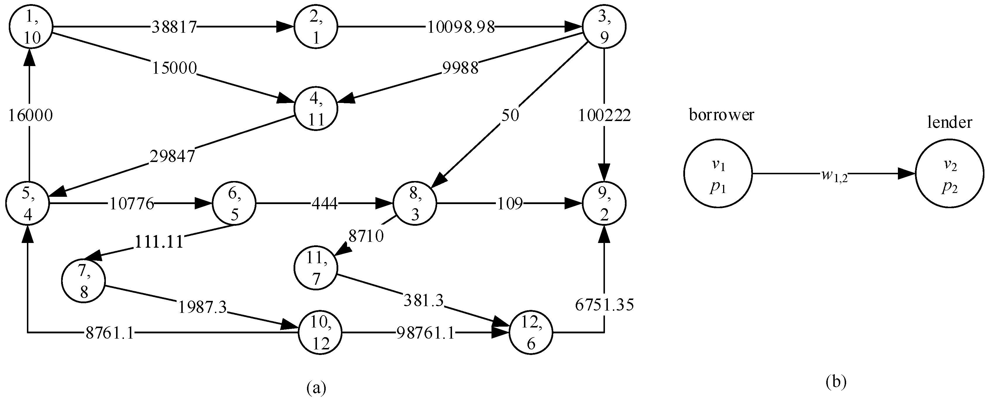
This problem stems from removing the dependency chain in weighted dependency graph [18] and debt chain in financial field. Taking debt chain as an example, the debt relationship among enterprises can be formulated as a weighted digraph, as defined above. In a graph , (1) each vertex stands for an enterprise; (2) each arc stands for a debt relationship between corresponding enterprises and means owes ; (3) associated with is the amount of debt of corresponding enterprises; and, (4) of vertex represents the importance of the corresponding enterprises, and the smaller has the higher priority. This kind of digraph is called a debt graph for convenience. Figure 1 illustrates an example including 12 enterprises. Debt cycle is a simple directed cycle in a given debt graph. It is very useful to solve the debt problem, because the enterprises belonging to a debt cycle can solve their debts without transferring capital.
4. Cycle Detection and Removal with Vertex Priority
Algorithm 1 shows the sketch of the proposed algorithm, and its details are given next.
| Algorithm 1. Detect and Remove Cycles of a Weighted Digraph |
| Step1: Simplify . |
| Step2: Divide into strongly connected components. |
| Step3: Detect, output and remove cycles of each strongly connected component. |
4.1. Graph Simplification
In Algorithm 1, line 1 simplifies the given graph by deleting the vertices and arcs that do not belong to any cycle. This step aims to decrease the scale of the graph, especially when is sparse. In fact, many graphs derived from real world are sparse [19]. Table 1 shows seven digraphs taken from SNAP (Stanford Network Analysis Platform) [20]. We can see that more than 50% of vertices having zero in- or out-degree. The debt graph is sparser than these graphs, as shown in Section 5.3.
Proposition 1.
Given a digraph , a vertex does not belong to any cycle if its out-degree or in-degree is 0.
According the above proposition, Algorithm 2 shows the simplification process. It first gets the in- and out-degrees of vertices (lines 2–5). The while loop (lines 7–18) repeats deleting vertices of or , and their corresponding arcs. Lines 8~14 find the first vertex satisfying Proposition 1. If such a vertex exists (line 15), it calls Algorithm 3 to delete this vertex. Algorithm 3 uses two for loops to delete the arcs associated with (lines 2–5 and 6–9) and itself (line 10).
| Algorithm 2. Simplify a Weighted Digraph | |
| 1. | Function Simplify() |
| 2. | for all do |
| 3. | in degree of |
| 4. | out degree of |
| 5. | end for |
| 6. | |
| 7. | while do |
| 8. | |
| 9. | for to do |
| 10. | if then |
| 11. | |
| 12. | break |
| 13. | end if |
| 14. | end for |
| 15. | if then |
| 16. | Delete() |
| 17. | end if |
| 18. | end while |
| 19. | return |
| 20. | end function |
| Algorithm 3. Delete a Vertex from a Weighted Digraph | |
| 1. | Function Delete(, ) |
| 2. | for all do |
| 3. | |
| 4. | |
| 5. | end for |
| 6. | for all do |
| 7. | |
| 8. | |
| 9. | end for |
| 10. | |
| 11. | end function |
4.2. Cycle Detection
Proposition 2.
Given a digraph , if is a directed cycle, then these vertices belong to the same strongly connected components of .
This is the basis of step 2 of Algorithm 1. There are several efficient algorithms to calculate strongly connected components (SCCs) of a digraph, so we do not discuss the detail of step 2 of Algorithm 1. After SCCs are obtained, the cycles can be detected in each SCC. The cycle calculation is the core of Algorithm 1.
Because the problem needs visit the vertices according their priorities, cycle should be detected using DFS. For large-scale graphs, the recursive DFS will cause out-of-memory exception, so we need an iterative version. The following data structures are adopted.
Stack is used to store the visited sequence of vertices. Its interfaces include:
- Push() to push into .
- Pop() to pop an element of .
- Peek() to return the top element of without popping out it.
- Search() to return the index of in , and it returns −1 if is not in .
- Clear() to clear the to empty.
- SubList() to return the sub-sequence of from index to ().
- IsEmpty() to return false if is not empty, and return true if is empty.
Key-value pair table is applied to record each neighbor vertex of a visited vertex is visited or not. As shown in Figure 2, each key () is a vertex that is unique in the whole table. Each has a list of values, and each value is either 0 or 1 representing the corresponding neighboring vertex of is unvisited or not. It has the following interfaces:
- Clear() to reset all values of key to 0.
- Sum() to return the sum of values of key . The sum represents the number of neighboring vertices have been visited until now.
- GetFirst() to return the first unvisited neighboring vertex of .
- Set() to set the value of neighboring vertex of to 1.
Minimum heap is applied to store vertices based on their priorities, due to the high-efficiency of sorting and deleting members in heap. It only has one function, GetFirst(H), to get the vertex of the highest priority.
Algorithm 4 gives the cycle detection algorithm. It is a multi-threading parallel algorithm. Line 2 forks threads, and all of the threads run in parallel (line 4). Each thread gets an SCC (line 5), and calls Fun to detect and remove cycles (line 6).
The set of vertices is stored in a minimum heap H. The outer while loop (lines 12~40) detects cycles starting from each vertex of . Lines 13~17 initialize variables. For a given vertex, , the inner while loop (lines 18~36) detects all of the cycles including . Let be the top element of . If all its neighbor vertices are visited (line 20), pop it out and clear the status of all its neighbor vertices. Otherwise, get the first unvisited neighbor vertex of and visit it. In further, if is not in (line 27), is pushed into . If is in and (line 29), than the sub-list of from to the top element is a cycle. If cannot find any cycle, delete it from graph (line 38).
| Algorithm 4. Detect Cycles of a Weighted Directed Graph | |
| 1. | Function DetectCycle() |
| 2. | Fork K threads |
| 3. | |
| 4. | for each thread do in parallel |
| 5. | the next SCC to detect and remove cycle |
| 6. | Fun() |
| 7. | end for |
| 8. | return |
| 9. | end function |
| 10. | Function Fun() // is a SCC of , is in heap H |
| 11. | |
| 12. | while do |
| 13. | GetFirst(H) |
| 14. | Clear() |
| 15. | Clear() |
| 16. | Push() |
| 17. | flag false |
| 18. | while (flag=false and isEmpty()=false) |
| 19. | Peek() |
| 20. | if |sum| then |
| 21. | Pop() |
| 22. | Clear() |
| 23. | else |
| 24. | GetFirst() |
| 25. | Set() |
| 26. | k=Search() |
| 27. | if then |
| 28. | Push() |
| 29. | else if then |
| 30. | SubList()// is a cycle |
| 31. | |
| 32. | RemoveCycle(,) |
| 33. | flag true |
| 34. | end if |
| 35. | end if |
| 36. | end while |
| 37. | if flag=false then |
| 38. | Delete() |
| 39. | end if |
| 40. | end while |
| 41. | return |
| 42. | end function |
When a cycle is detected, it should be removed at once using RemoveCycle (line 32) shown in Algorithm 5. The first for loop (lines 3–7) finds the cycle weight. The second for loop (lines 8–20) decreases all of the arc weights of by . If the weight of an arc becomes 0, delete this arc (line 11). In further, if the in-degree or out-degree of a vertex becomes 0, delete this vertex (lines 13 and 16).
| Algorithm 5. Remove a Cycle | |
| 1. | Function RemoveCycle(,)//, |
| 2. | |
| 3. | for to do |
| 4. | if then |
| 5. | |
| 6. | end if |
| 7. | end for |
| 8. | for to do |
| 9. | |
| 10. | |
| 11. | if then |
| 12. | |
| 13. | if then |
| 14. | Delete() |
| 15. | end if |
| 16. | if then |
| 17. | Delete() |
| 18. | end if |
| 19. | end if |
| 20. | end for |
| 21. | end function |
Proposition 3.
Given a strongly connected component , Algorithm 4 can terminate with .
Proof.
Let be the vertex with the highest priority in SCC , i.e., is the minimal. From , DFS is used to visit this SCC. Let be the current visiting vertex.
Case 1. has no outgoing arc or all its neighbor vertices are visited in previous steps. In this case, , and should be popped out from .
Case 1-1. If , becomes empty, so the inner while (line 18) exits and flag=false. This result means no cycle can be detected from , so is deleted (line 38).
Case 1-2. If , the inner while (line 18) goes on checking the top element of .
Case 2. has at least one unvisited outgoing arc. In this case, we select one unvisited neighbor vertex to continue searching.
Case 2-1. If , a cycle is detected (line 29). This cycle is removed by Algorithm 5. Because equals to at least one arc's weight, Algorithm 5 deletes at least one arc. Finally, flag=true, and the inner while loop exits.
Case 2-2. If is not visited, is pushed into and while loop continues.
Case 2-3. If is in stack but , it continues finding the next vertex to visit.
Note that Case 1-2, Case 2-2 and Case 2-3 will fall into Case 1-1 or Case 2-1 finally, so each iteration of outer while loop deletes an arc or vertex at least. Therefore, when Algorithm 4 finishes.
Remark 1.
Algorithm 4 cannot detect all cycles of a given SCC, because a cycle may be broken when another one is removed.
4.3. Time Complexity Analysis
Let be, respectively, the average in-degree and out-degree of vertices.
In Algorithm 2, the for consumes to compute the in- and out-degree of all vertices. When no vertex can be deleted, the while only needs to scan all vertices. When only one vertex can be deleted in each iteration, it consumes .
Algorithm 3 is very simple, whose time complexity is .
Let be the length of cycle as the input of Algorithm 5. The first for consumes . If only one arc can be deleted, the second for consumes . In the worst case, arcs of this cycle are all deleted, then the second for consumes .
For function Fun() of Algorithm 4, in the worst case, each iteration of the inner while detects a cycle, and each cycle only deletes one arc using Algorithm 5, so this function calls times Algorithm 5. Obviously, the longest cycle is of length , and the shortest one is of length 2, so the average length of cycles is
If has SCCs, each thread deals with SCCs on average. Therefore, the worst time complexity is .
The time complexity of Algorithm 1 is the sum of Algorithms 2–4. In the worst case, the digraph has only one SCC, so its time complexity is .
4.4. An Example
Taking Figure 1 as an example, vertex 9 is deleted in first for its out-degree is 0, and its adjacent arcs are deleted too. Vertices 12, 11, and 8 are deleted in succession.
After simplification, the remaining vertices are all in one SCC. Vertex 2 becomes the first one to find cycle due its highest priority. Starting from vertex 2, vertices 3, 4, 5 are visited successively. Between two adjacent vertices of 5, 6 is chosen as the next vertex due to its higher priority. After visiting 7, 10 and 5, a cycle (5, 6, 7, 10) is detected. Since it does not contain 2, so the algorithm backtracks and visits 1, and then visits 2 to detect a cycle {1, 2, 3, 4, 5}. This cycle’s weight . After calling Algorithm 3, the arc is deleted. Repeat the above process, cycles (5, 6, 7, 10) and (1, 4, 5) are detected and removed, and then the graph is cycle-free. In one word, Algorithm 4 can find 3 cycles in Figure 1.
5. Experiments and Analysis
The experiments are performed on a PC with Inter Core i7-5500U @ 2.40GHz CPU (dual-core), 6GB memory, Windows 7 operating system. The programs are coded with Java in Eclipse, and we set the upper-bound stack size to 4GB. The following versions of algorithm are compared:
- Recursion without simplification (RWOS). It detects cycle recursively without simplification. It is the popular algorithm used by many literatures.
- Recursion with simplification (RWS). It detects cycle recursively after simplification.
- Iteration without simplification (IWOS). It detects cycle iteratively without simplification.
- Iteration with simplification (IWS). It detects cycle iteratively after simplification.
- Multi-thread parallel IWS (MPIWS). It detects cycle in parallel with IWS using multi-threads.
In order to compare their performance, we define as the ratio of execution time between algorithm A () and B (). Obviously, means that algorithm A is better than B. Considering the algorithms to be compared, we define
5.1. Experiments with Randomly Generated Digraphs
First, we generate 100 digraphs randomly to analyze the performance of the above algorithms. Each kind of digraph has different number of vertices and arcs. These digraphs have vertices, and the average out degree of vertices is 1 to 10 in step of 1. For each kind of digraph, we generate 10 different digraphs, and each algorithm runs 10 times for each digraph. The results are average over these 10 runs.
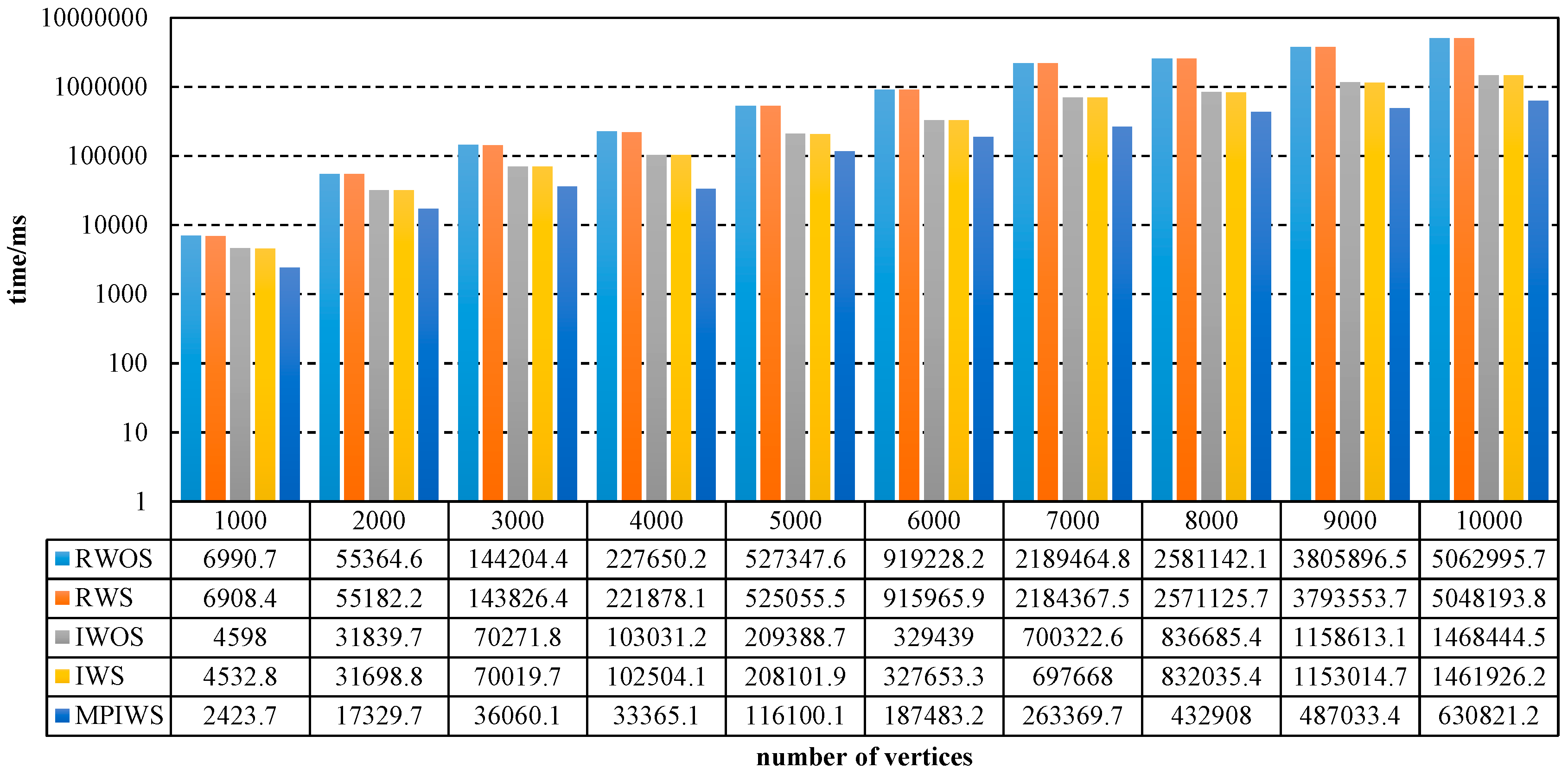
As shown in Figure 3, the iterative algorithm is significantly better than recursive algorithm because and , and and decrease while the number of vertices increases. and are almost the same when is the same. When , , and . When , . Figure 3 also shows that simplification cannot reduce execution time effectively. For a different number of vertices, , and . MPIWS outperforms IWS in further due to .
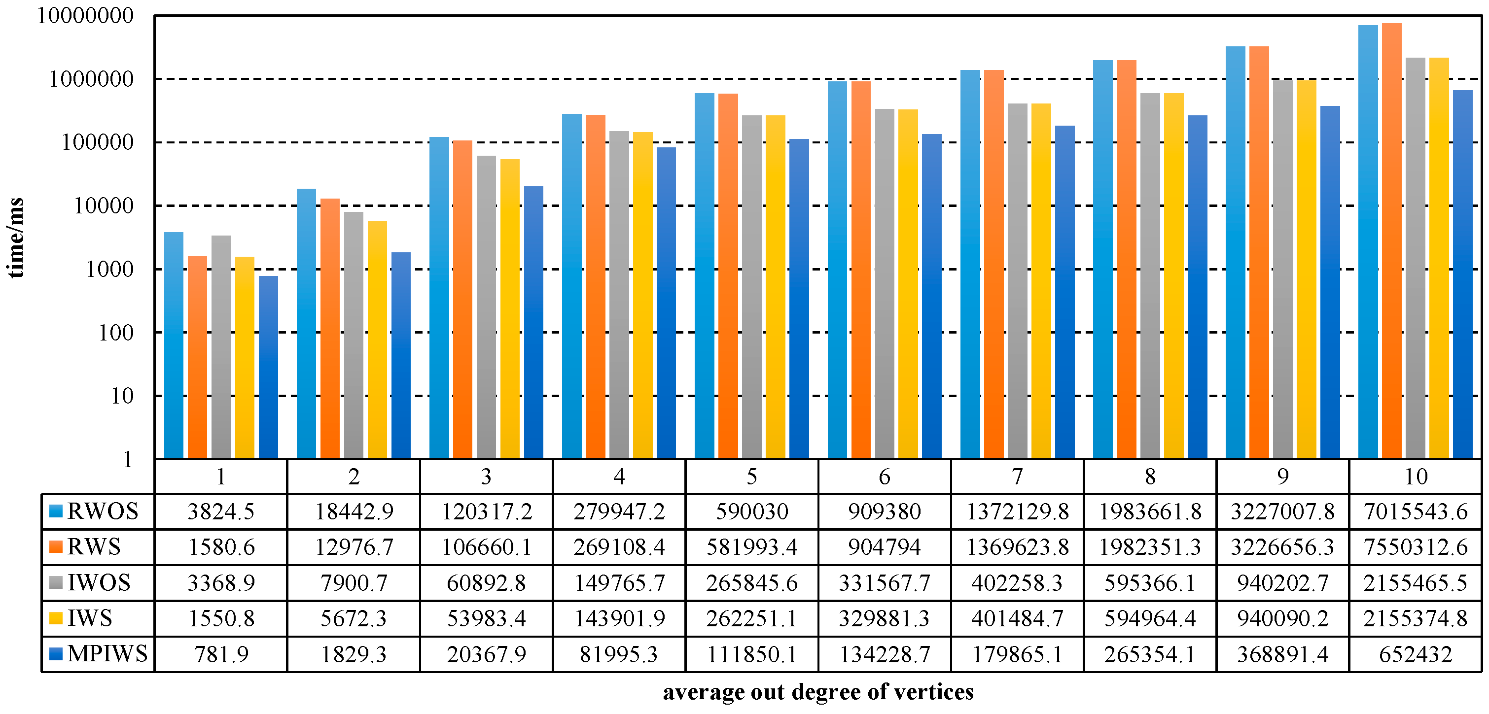
Figure 4 shows that the iterative algorithm outperforms the recursive version when the average degree of vertices is the same, and and decrease while the average out-degree of vertices increases. When out-degree is 1, , . When out-degree is 10, , . MPIWS also outperforms IWS in this figure, and .
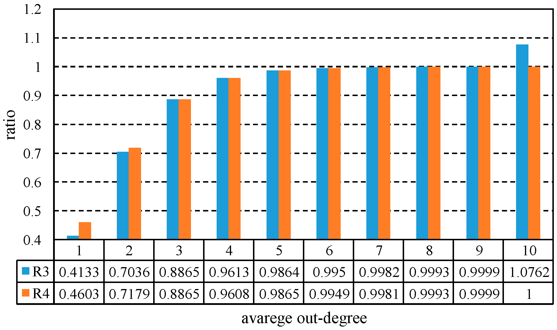
Figure 4 shows that simplification has much effect on the performance of these algorithms. Figure 5 shows the numeric results of and , and increase rapidly when out-degree increases from 1 to 3, but they change a little when out-degree is larger than 3. Specially, and equal to or are greater than 1 when the average degree is 10, which means that the simplification has no effect on the algorithm’s efficiency.
In fact, when the average degree is relatively small, a large portion of vertices and arcs will be deleted by Algorithm 2, as shown in Figure 6. When the average degree is 1, the residual vertices and arcs are only about 0.7% of original graph. When the degree is 2, this ratio increases to 63% rapidly. Only less than 10% of vertices and arcs can be deleted when the average degree is larger than 3.
5.2. Experiments with SNAP Datasets
RWS, IWS, and MPIWS are used to detect and remove cycles of seven digraphs from SNAP datasets, and Table 2 shows the results. RWS cannot complete correctly for the last five graphs. The stack of RWS reaches 4GB before RWS can solve the problem, so it leads to out-of-memory exception in Java. IWS and MPIWS can solve the problem correctly, but MPIWS outperforms IWS because .
5.3. Experiments with Real Dept Graphs
In order to analyze the performance in real application, we utilize them for a real debt graph. The debt data comes from Qingdao YouRong Development Co., Ltd., in Shandong Province, China. This graph has 7692 vertices and 8737 arcs, so the average out-degree of each vertex is about 1.14. After simplification, the graph only has 184 vertices and 345 arcs, namely only 2.39% vertices and 3.95% arcs are saved after simplification. The simplified graph is shown in Figure 7. This figure is drawn by Pajek.
Figure 8 presents the execution times of RWOS, RWS, IWOS, IWS, and MPIWS to solve the real debt graph. We can see that , which shows simplification, iteration, and parallelism improves the performance when compared with traditional recursive algorithms without simplification.
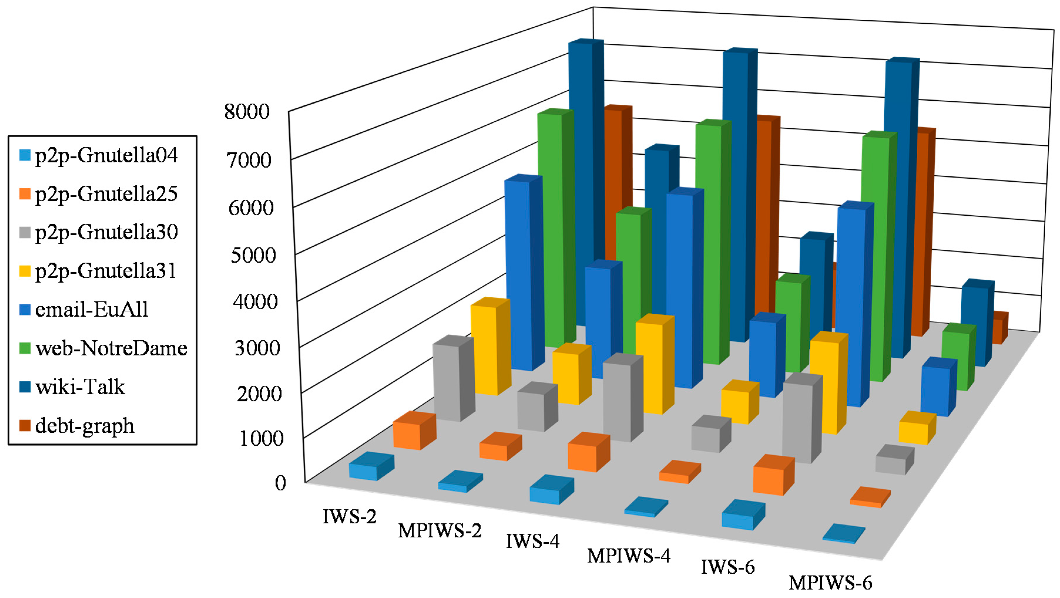
5.4. Performance Comparisons on Different Computers
We compare the speedups of IWS and MPIWS on the follow CPUs: Intel Core i7-7700 (quad-cores), Intel Core i7-5820K (six-cores), and the results are shown in Figure 9. The main memory is still 6GB. Since RWS still cannot solve all graphs, we only compare IWS and MPIWS. In Figure 9, IWS-2, IWS-4, and IWS-6 are the execution time of IWS on i7-5500U, i7-7700, and i7-5820K, respectively. MPIWS-2, MPIWS-4, and MPIWS-6 are the execution time of MPIWS on i7-5500U, i7-7700, and i7-5820K, respectively. The “debt-graph” is the graph used in Section 5.3.
Figure 9 shows that the increasement of cores has little influence on IWS. However, MPIWS changes a lot using different CPU. TMPIWS using i7-7700 is about 59.1~66.3% of TMPIWS using i7-5500U, and TMPIWS using i7-5820K is about 41.1~67.4% of TMPIWS using i7-7700. This figure also shows that R5 decreases with an increase of cores. Using i7-5500U, i7-7700, and i7-5820K, the values of R5 are, respectively, , , and .
6. Conclusion and Discussion
Many real-world scenarios and applications can be modeled as a graph, and many problems need to detect cycles. Derived from cycle detection and removal problem in debt graph, this paper defines a new problem that detects cycle according to the vertex priority, and removes cycles according to arc weight. A multi-threading parallel and iterative algorithm is proposed to solve this problem. Iteration is applied to replace recursion and to avoid out-of-memory exception, and multi-thread is applied to improve the efficiency. The experiments exhibit that the iterative algorithm can be run on a single commodity PC to solve the large-scale graph, and parallel algorithm outperforms sequential algorithm obviously. In further, the proposed algorithm uses simplification to reduce the scale of graph. The experiments show that the execution efficiency is improved significantly by simplification when there are many vertices having 0 in- or out-degree.
Generally, iteration outperforms recursion while solving a same problem, but simplification is only applicable to sparse graph. If the graph is not sparse, line 2 of Algorithm 1 can be deleted. Moreover, commodity PCs cannot solve the problem, even use of MPIWS in case of the graph is too large, so parallel algorithms depending on computer cluster must be applied, such as the algorithms proposed in [14,21,22].
Acknowledgments
This work is supported by the National Key Research and Development Program of China Grant No. 2017YFC0804406 and 2017YFB0202001, and the Open Project of Shandong Provincial Key Laboratory of Computer Networks, Grant No. SDKLCN-2015-03.
Author Contributions
H. Cui conceived and designed the experiments; J. Niu performed the experiments; C. Zhou and M. Shu analyzed the data; H. Cui wrote the paper.
Conflicts of Interest
The authors declare no conflict of interest.
References
- Kühn, D.; Osthus, D. A survey on hamilton cycles in directed graphs. Eur. J. Combin. 2012, 33, 750–766. [Google Scholar] [CrossRef]
- Silva, J.L.C.; Rocha, L.; Silva, B.C.H. A new algorithm for finding all tours and hamiltonian circuits in graphs. IEEE Lat. Am. Trans. 2016, 14, 831–836. [Google Scholar] [CrossRef]
- Lv, X.; Zhu, D. An approximation algorithm for the shortest cycle in an undirected unweighted graph. In Proceedings of the International Conference on Computer, Mechatronics, Control and Electronic Engineering, Changchun, China, 24–26 August 2010; IEEE: New York, NY, USA, 2010; pp. 297–300. [Google Scholar]
- Yuster, R. A shortest cycle for each vertex of a graph. Inform. Process. Lett. 2011, 111, 1057–1061. [Google Scholar] [CrossRef]
- Paulusma, D.; Yoshimoto, K. Cycles through specified vertices in triangle-free graphs. Discuss. Math. Gr. Theory 2007, 27, 179–191. [Google Scholar] [CrossRef]
- Li, B.; Zhang, S. Heavy subgraph conditions for longest cycles to be heavy in graphs. Discuss. Math. Gr. Theory 2016, 36, 383–392. [Google Scholar] [CrossRef]
- Li, B.; Xiong, L.; Yin, J. Large degree vertices in longest cycles of graphs, I. Discuss. Math. Gr. Theory 2016, 36, 363–382. [Google Scholar] [CrossRef]
- Gerbner, D.; Keszegh, B.; Palmer, C.; Patkos, B. On the Number of Cycles in a Graph with Restricted Cycle Lengths. Available online: https://arxiv.org/abs/1610.03476 (accessed on 9 October 2017).
- Sankar, K.A.; Sarad, V. A time and memory efficient way to enumerate cycles in a graph. In Proceedings of the International Conference on Intelligent and Advanced Systems, Kuala Lumpur, Malaysia, 25–28 November 2007; IEEE: New York, NY, USA, 2007; pp. 498–500. [Google Scholar]
- Haeupler, B.; Kavitha, T.; Mathew, R.; Sen, S.; Tarjan, R.E. Incremental Cycle Detection, Topological Ordering, and Strong Component Maintenance. Available online: https://arxiv.org/abs/1105.2397 (accessed on 9 October 2017).
- Bender, M.A.; Fineman, J.T.; Gilbert, S.; Tarjan, R.E. A new approach to incremental cycle detection and related problems. ACM Trans. Algorithms 2016, 12. [Google Scholar] [CrossRef]
- Reif, J.H. Depth-first search is inherently sequential. Inform. Process. Lett. 1985, 20, 229–234. [Google Scholar] [CrossRef]
- Karimi, M.; Banihashemi, A.H. Message-passing algorithms for counting short cycles in a graph. IEEE Trans. Commun. 2013, 61, 485–495. [Google Scholar] [CrossRef]
- Rocha, R.C.; Thatte, B.D. Distributed cycle detection in large-scale sparse graphs. In Proceedings of the Simpósio Brasileiro de Pesquisa Operacional, Pernambuco, Brazil, 25–28 August 2015; XLVII SBPO: Pernambuco, Brazil, 2015; pp. 1–11. [Google Scholar]
- Malewicz, G.; Austern, M.H.; Bik, A.J.C.; Dehnert, J.C.; Horn, I.; Leiser, N.; Czajkowski, G. Pregel: A system for large-scale graph processing. In Proceedings of the ACM SIGMOD International Conference on Management of Data, Indianapolis, IN, USA, 6–11 June 2010; ACM: New York, NY, USA, 2010; pp. 135–146. [Google Scholar]
- Gonzalez, J.E.; Xin, R.S.; Dave, A.; Crankshaw, D.; Franklin, M.J.; Stoica, I. GraphX: Graph processing in a distributed dataflow framework. In Proceedings of the 11th USENIX Symposium on Operating Systems Design and Implementation, Broomfield, CO, USA, 6–8 October 2014; USENIX: Berkeley, CA, USA, 2014; pp. 599–613. [Google Scholar]
- Salihoglu, S.; Widom, J. GPS: A graph processing system. In Proceedings of the 25th International Conference on Scientific and Statistical Database Management, Baltimore, MD, USA, 29–31 July 2013; ACM: New York, NY, USA, 2013; pp. 1–31. [Google Scholar]
- Féray, V. Weighted dependency graphs. Available online: https://arxiv.org/abs/1605.03836 (accessed on 9 October 2017).
- McLendon, W.; Hendrickson, B.; Plimpton, S.J.; Rauchwerger, L. Finding strongly connected components in distributed graphs. J. Parallel Distrib. Comput. 2005, 65, 901–910. [Google Scholar] [CrossRef]
- Leskovec, J.; Sosic, R. SNAP: A general-purpose network analysis and graph-mining library. ACM Trans. Intell. Syst. Technol. 2016, 8. [Google Scholar] [CrossRef] [PubMed]
- Seidl, T.; Boden, B.; Fries, S. CC-MR—Finding connected components in huge graphs with MapReduce. In Proceedings of the Joint European Conference on Machine Learning and Knowledge Discovery in Databases, Bristol, UK, 24–28 September 2012; Springer: Berlin/Heidelberg, Germany, 2014; pp. 458–473. [Google Scholar]
- Slota, G.M.; Rajamanickam, S.; Madduri, K. BFS and coloring-based parallel algorithms for strongly connected components and related problems. In Proceedings of the IEEE 28th International Parallel and Distributed Processing Symposium, Phoenix, AZ, USA, 19–23 May 2014; IEEE: New York, NY, USA, 2014; pp. 550–559. [Google Scholar]
Figure 1.
An example of debt graph. (a) A debt graph; (b) legend.

Figure 2.
An example of key-vale pair table.
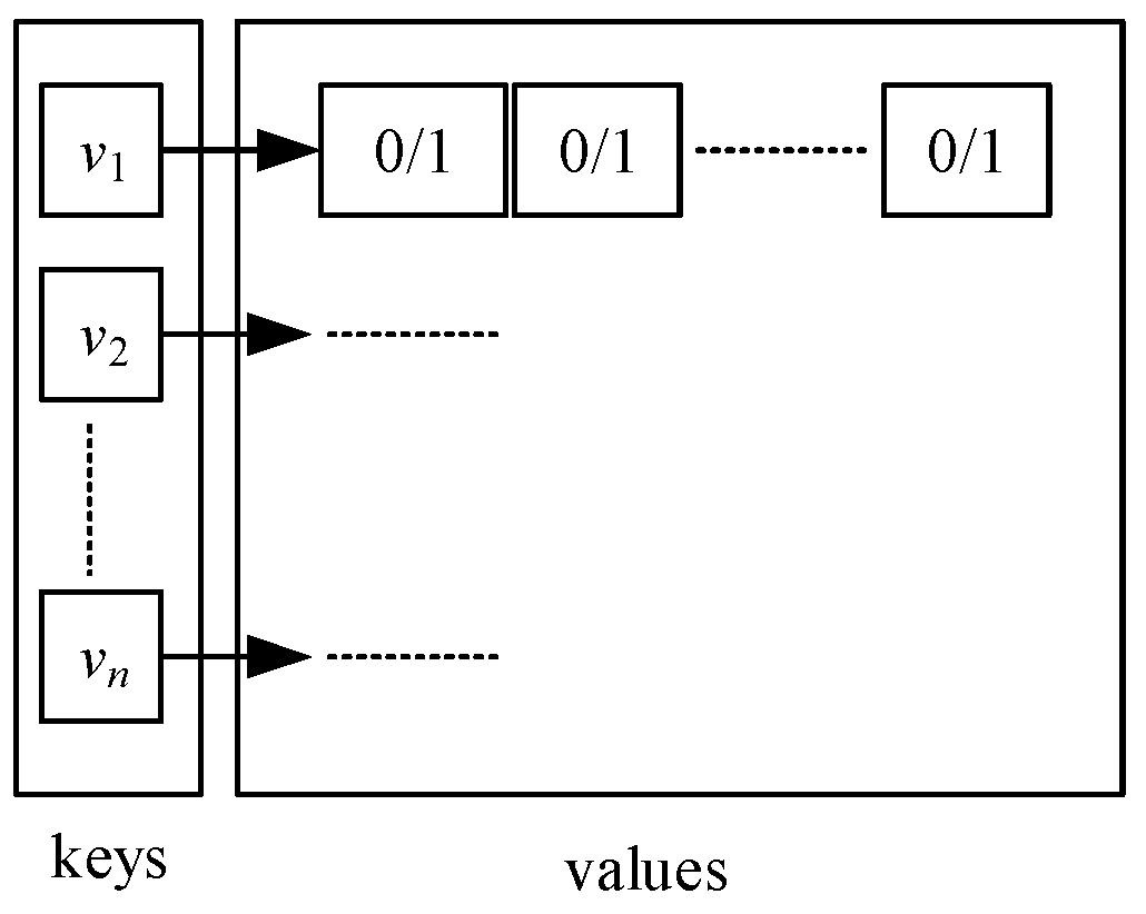
Figure 3.
Impacts of number of vertices on execution time of each algorithm.

Figure 4.
Impacts of average degree of vertices on execution time of each algorithm.

Figure 5.
and under different out-degree.

Figure 6.
Ratio of number of residual vertices and arcs after simplification.
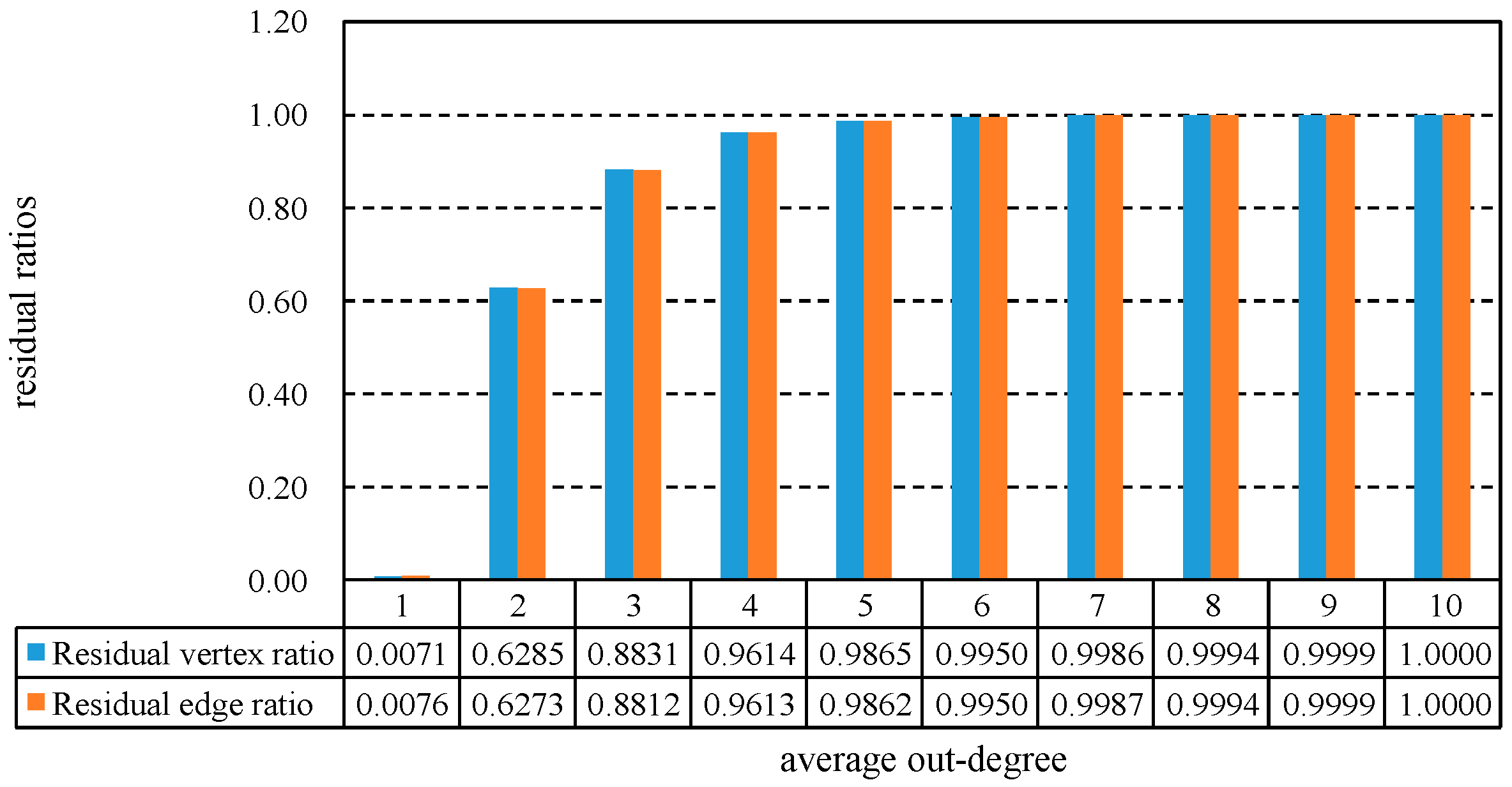
Figure 7.
A real debt graph after simplification.
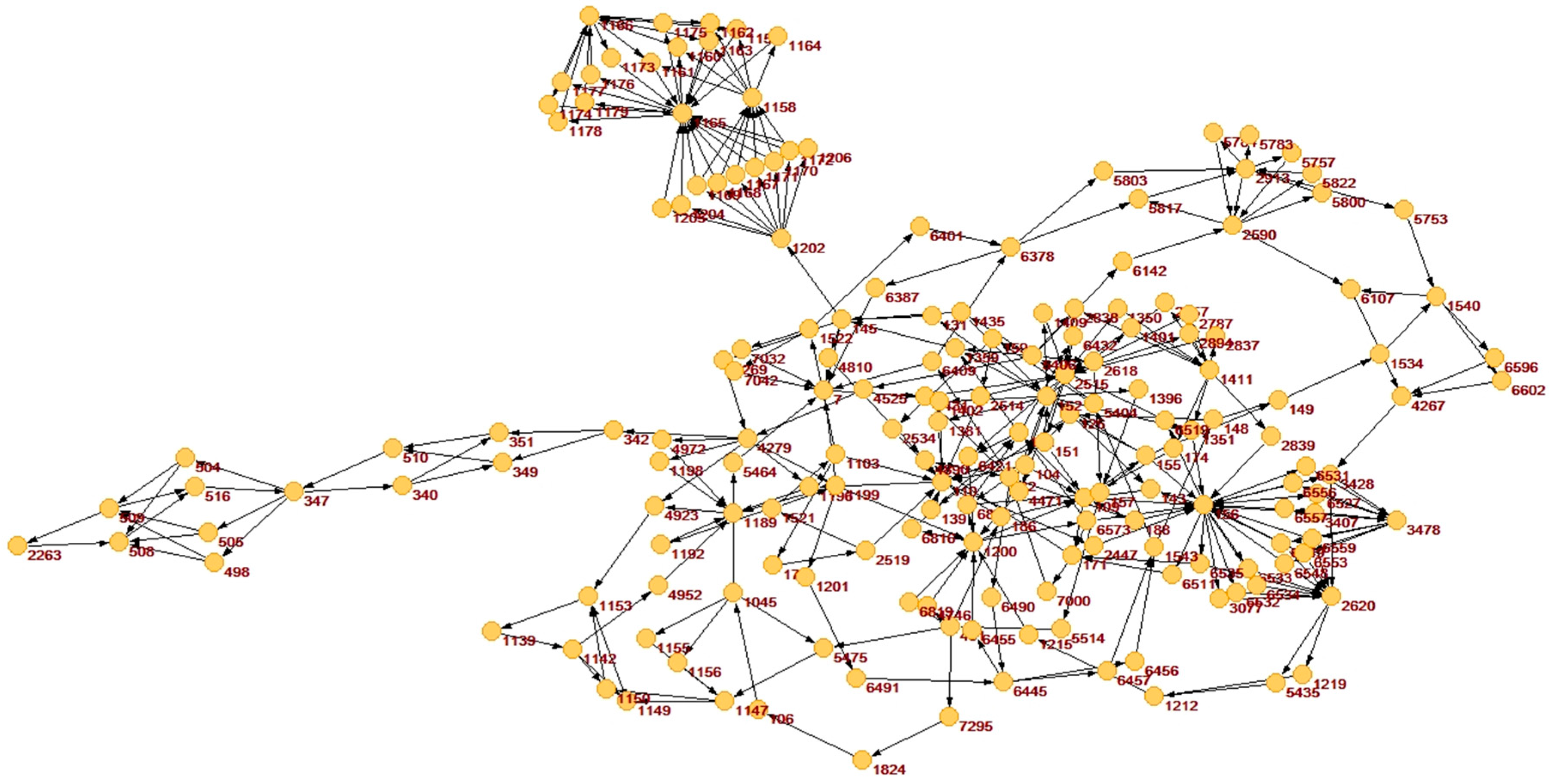
Figure 8.
Execution time of four algorithms.
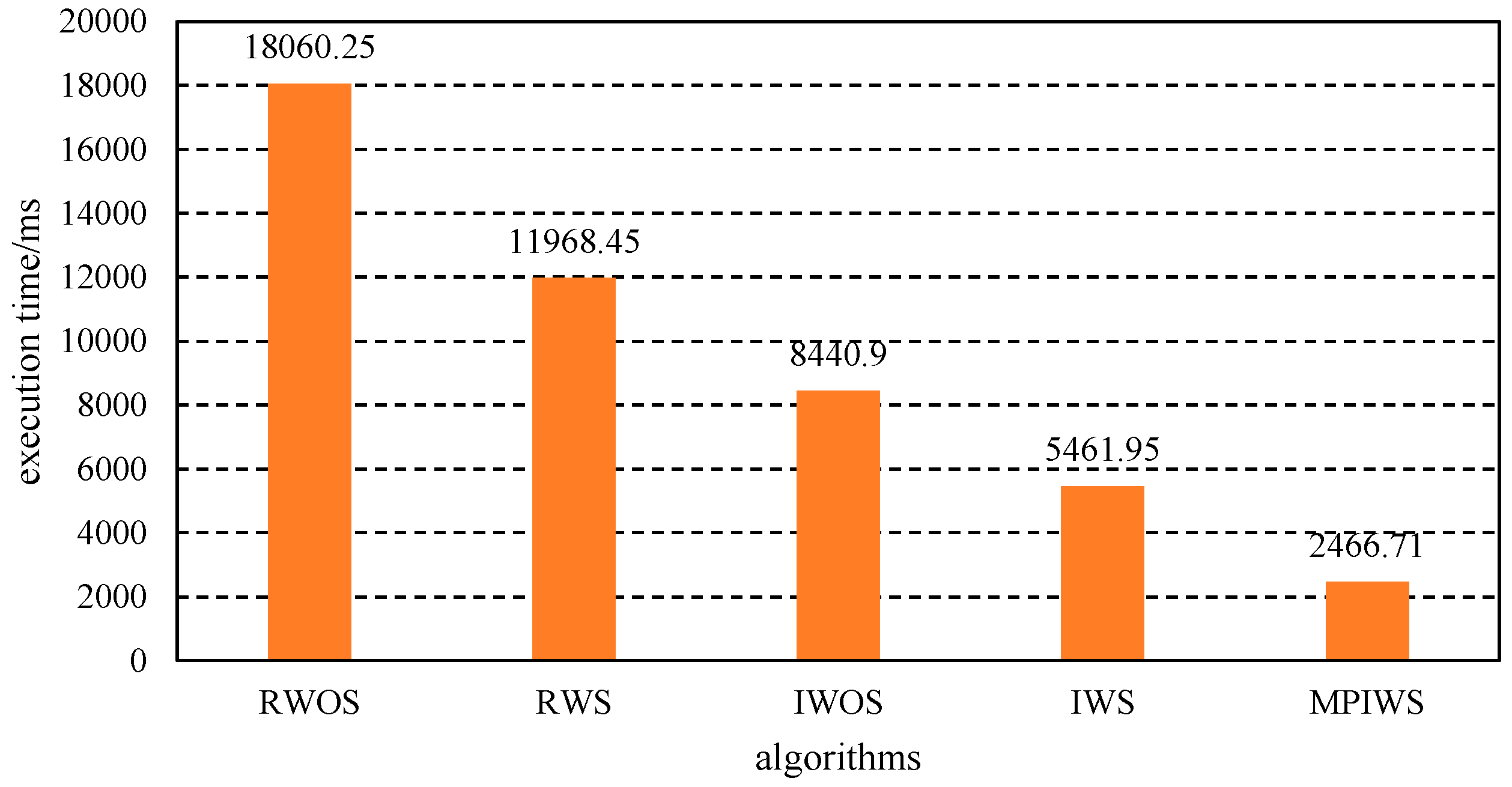
Figure 9.
Execution time of different algorithms on different CPU.


Table 1.
The sparse characteristic of Stanford network analysis platform (SNAP) graphs.
| Graph Name | p2p-Gnutella04 | p2p-Gnutella25 | p2p-Gnutella30 | p2p-Gnutella31 | Email-EuAll | Web-NotreDame | Wiki-Talk |
|---|---|---|---|---|---|---|---|
| 10,876 | 22,687 | 36,682 | 62,586 | 265,214 | 325,729 | 2,394,385 | |
| 39,994 | 54,705 | 88,328 | 147,892 | 420,045 | 1,497,134 | 5,021,410 | |
| ratio 1 | 54.80% | 74.06% | 74.12% | 74.29% | 95.79% | 57.65% | 94.88% |
1 “ratio” is the ratio of vertices of out- or in-degree 0 to .
Table 2.
Performance Analysis of Algorithms (time unit: ms. ‘-‘ means it has no value).
| Graph Name | p2p-Gnutella04 | p2p-Gnutella25 | p2p-Gnutella30 | p2p-Gnutella31 | email-EuAll | Web-NotreDame | Wiki-Talk |
|---|---|---|---|---|---|---|---|
| 355.5179 | 615.3466 | - | - | - | - | - | |
| 315.4235 | 592.1235 | 1804.2942 | 2181.8719 | 4788.6087 | 6075.5061 | 7560.0935 | |
| 147.0574 | 342.7287 | 891.0342 | 1238.7748 | 2798.9455 | 3680.5876 | 4907.7557 | |
| 0.4662 | 0.5788 | 0.4938 | 0.5678 | 0.5845 | 0.6058 | 0.6492 |
© 2017 by the authors. Licensee MDPI, Basel, Switzerland. This article is an open access article distributed under the terms and conditions of the Creative Commons Attribution (CC BY) license (http://creativecommons.org/licenses/by/4.0/).
Share and Cite
MDPI and ACS Style
Cui, H.; Niu, J.; Zhou, C.; Shu, M. A Multi-Threading Algorithm to Detect and Remove Cycles in Vertex- and Arc-Weighted Digraph. Algorithms 2017, 10, 115. https://doi.org/10.3390/a10040115
AMA Style
Cui H, Niu J, Zhou C, Shu M. A Multi-Threading Algorithm to Detect and Remove Cycles in Vertex- and Arc-Weighted Digraph. Algorithms. 2017; 10(4):115. https://doi.org/10.3390/a10040115
Chicago/Turabian StyleCui, Huanqing, Jian Niu, Chuanai Zhou, and Minglei Shu. 2017. "A Multi-Threading Algorithm to Detect and Remove Cycles in Vertex- and Arc-Weighted Digraph" Algorithms 10, no. 4: 115. https://doi.org/10.3390/a10040115
Note that from the first issue of 2016, this journal uses article numbers instead of page numbers. See further details here.