Remote Sensing Image Enhancement Based on Non-Local Means Filter in NSCT Domain

1
College of Communication Engineering, Jilin University, Changchun 130012, China
2
Department of Electronic Information, Zhuhai College of Jilin University, Zhuhai 519041, China
3
College of Information Science and Engineering, Xinjiang University, Urumqi 830046, China
*
Author to whom correspondence should be addressed.
Algorithms 2017, 10(4), 116; https://doi.org/10.3390/a10040116
Submission received: 17 September 2017
/
Revised: 27 September 2017
/
Accepted: 3 October 2017
/
Published: 11 October 2017
Abstract
:In this paper, a novel remote sensing image enhancement technique based on a non-local means filter in a nonsubsampled contourlet transform (NSCT) domain is proposed. The overall flow of the approach can be divided into the following steps: Firstly, the image is decomposed into one low-frequency sub-band and several high-frequency sub-bands with NSCT. Secondly, contrast stretching is adopted to deal with the low-frequency sub-band coefficients, and the non-local means filter is applied to suppress the noise contained in the first high-frequency sub-band coefficients. Thirdly, the processed coefficients are reconstructed with the inverse NSCT transform. Finally, the unsharp filter is used to enhance the details of the image. The simulation results show that the proposed algorithm has better performance in remote sensing image enhancement than the existing approaches.
1. Introduction
Due to the limitations of image acquisition devices and external factors, the resolution of remote sensing images is not very satisfactory, so image enhancement techniques play a very important role in image analysis [1,2]. The purpose of image enhancement is to highlight the useful features of the image [3,4], and image enhancement methods are widely used in areas such as atmospheric sciences [5], medical image processing [6,7], satellite image analysis [8,9], and remote sensing [10].
So far, image enhancement approaches can be divided into two categories: spatial domain and frequency domain. In terms of spatial domain enhancement, Histogram equalization (HE) is a widely used method to enhance images, but HE may result in the over-enhancement phenomenon of image processing, and make the image too dark in some regions [1,11]. In order to make up for the shortcomings of the HE method, some improved algorithms based on HE have been proposed, such as contrast limited adaptive histogram equalization (CLAHE) [12], brightness preserving bi-histogram equalization (BBHE) [13], dualistic sub-image histogram equalization (DSIHE) [14], exposure based sub-image histogram equalization (ESIHE) [15], etc. Gamma correction [16] is also a useful method to improve the contrast of digital images, and some improved techniques have been proposed based on this, such as adaptive gamma correction with weighting distribution (AGCWD) [17] and adaptive gamma correction for image enhancement [1]; these approaches have achieved good performance in image enhancement. With the research of image enhancement algorithms, image enhancement methods based on frequency domain transform came into being, with the most typical approach being wavelet transform [18]. Due to the good time-frequency localization and multi-resolution of wavelets, the wavelet has been widely used in texture analysis, image processing, and other fields. Arising from wavelet theory, some new frequency domain enhancement techniques have been proposed, such as curvelet transform [19] and contourlet transform [20]. However, the contourlet transform does not have translation invariance. Due to the existence of this shortcoming, the pseudo-Gibbs phenomenon can easily appear around the singular points in the image restoration. In order to deal with thise weakness, the nonsubsampled contourlet transform (NSCT) was proposed [21,22]. The NSCT transform has many merits such as time-frequency locality, multi-resolution, multi-direction, and anisotropy, which can sparsely represent the image. The NSCT has since been widely applied in image fusion and image enhancement [23,24]. In this paper, a novel remote sensing enhancement approach based on a non-local means filter in NSCT domain is proposed.
The reminder of this paper is expressed as follows: Section 2 introduces the theoretical methods adopted in this article, including the nonsubsampled contourlet transform and non-local means filter models; the implementation of the proposed approach is described in Section 3; the experimental results and discussions are offered in Section 4; and the conclusions of the proposed remote sensing image enhancement method are described in Section 5.
2. Theoretical Analysis
2.1. Nonsubsampled Contourlet Transform
Nonsubsampled contourlet transform (NSCT) is put forward on the basis of contourlet transform, and it is an overcomplete transformation. Though the structure of the NSCT transformation is similar to the contourlet transform, NSCT does not use the sampling link. NSCT is composed of the Nonsubsampled pyramid filter bank (NSPFB) and the Nonsubsampled directional filter bank (NSDFB) [25]; the corresponding structure is shown in Figure 1. NSCT is a transformation characterized by multi-scale, good spatial and frequency domain, shift-invariance and higher redundancy. NSCT transform first uses NSPFB to obtain the multi-scale decomposition of the input image, and then NSDFB is applied to decompose the obtained sub-band images in order to achieve the sub-band coefficients of different scales and different directions. Figure 2 is the flow chart of NSCT. The test image (zoneplate) is decomposed by NSCT as shown in Figure 3.
For the nonsubsampled pyramid (NSP) decomposition, the analytical filter {H0(z), H1(z)} and the integrated filter {G0(z), G1(z)} satisfy the Bezout identity. The corresponding equation is expressed as follows:
For the nonsubsampled directional filter bank, the analytical filter {U0(z), U1(z)} and the integrated filter {V0(z), V1(z)} also satisfy the Bezout identity. The corresponding formula is described as follows:
2.2. Non-Local Means Filter
Non-local means filter (NLM filter) is a very effective denoising method [26,27]. This algorithm makes full use of the redundant information in the image. It can eliminate the noise in the image and keep the details of the image to their maximum extent. In this paper, we assume that the input image is y, and the estimated value of the denoised image is x; I is the image domain, and i is an arbitrary pixel in the image domain. The gray value of i can be obtained by weighing the average of all pixels in the image. The corresponding formula is expressed as follows:
where w presents the similar weight of the pixels i and j. The value of this weight depends on y(Ni) and y(Nj). The formula for similar weight can be expressed as follows:
where y(Ni) is the gray vector value of the (2k + 1) × (2k + 1) window; h is a smoothing parameter; Ni and Nj represent square neighborhoods of the fixed size, same size centered on pixels i and j, respectively. In thise paper, we set h = 5, k = 2, w = 10.
3. Implementation of the Proposed Method
3.1. Contrast Stretching in Low-Frequency Sub-Band
The low-frequency component contains much of the background information of the image, and the contrast of the image can be enhanced by adjusting the coefficients of the low-frequency sub-band. In this paper, contrast stretching is applied to deal with the low-frequency component, and the corresponding formula is defined as follows [28]:
where ymax and ymin are the maximum and minimum values of gray image, respectively.
3.2. NLM Filter Denoising in High-Frequency Sub-Bands
The coefficients of the high-frequency sub-bands contain detailed information from the remote sensing images, but also contain a lot of noise. In this paper, the non-local means filter as described in Section 2.2 is adopted to suppress the noise in the first high-frequency sub-band, because it has the most noise. The other high-frequency sub-bands coefficients are not treated.
3.3. Steps of the Proposed Method
- Step 1
- The original image is decomposed into one low-frequency sub-band and several high-frequency sub-bands by NSCT transform.
- Step 2
- The low-frequency sub-band coefficients are processed with contrast stretching according to equation 7, and the noise of the first high-frequency sub-band coefficients is suppressed by the NLM filter according to equations 3–6.
- Step 3
- The adjusted coefficients are reconstructed with inverse NSCT transform.
- Step 4
- The reconstructed image is enhanced by the unsharp filter.
The flow chart of the proposed method is shown in Figure 4.
4. Results and Discussions
In this section, in order to demonstrate that the proposed approach is effective, many remote sensing images were tested using MATLAB 2016a. Four existing image enhancement methods were selected to compare with the proposed method, namely histogram equalization (HE) [29], exposure based sub-image histogram equalization (ESIHE) [15], feature-linking model for image enhancement (FLM) [30], and linking synaptic computation for image enhancement (LSCN) [31]. We used subjective and objective aspects to evaluate the image enhancement effects. In terms of the objective metrics, six evaluation metrics were applied, namely information entropy (H) [32], mean square error (MSE) [33], peak signal-to-noise ratio (PSNR) [34], gradient magnitude similarity deviation (GMSD) [35], mean absolute error (MAE) [36], and multi-scale structural similarity (MSSSIM) [37]. For the indicators of H, PSNR, and MSSSIM, larger values demonstrate a better enhancement of the image; for the other three metrics MSE, GMSD, and MAE, lower values demonstrate a better enhancement of the image. The data of the experimental results are shown in Table 1, Table 2, Table 3 and Table 4. In this article, the decomposition level of NSCT is 3, and the directions in the scales from coarser to finer are 8, 16, 16. We used the 9-7 filter and dmaxflat7 as the NSPFB filter and NSDFB filter, respectively.
4.1. Subjective Analysis
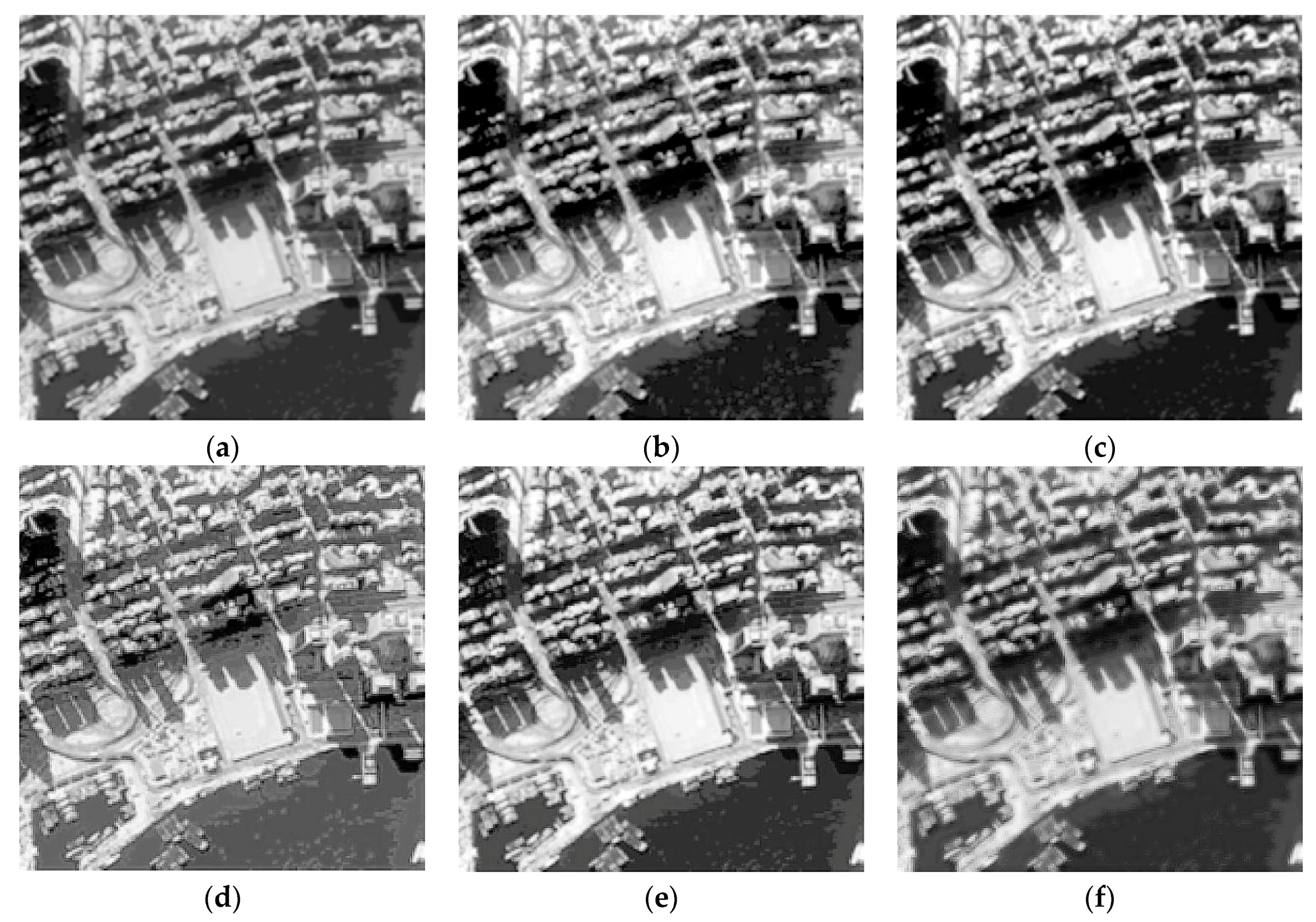
Figure 5 is the enhanced result of the five image enhancement techniques simulated on Image 1. The size of the original image is 556 × 556. Figure 5a is the original image; Figure 5b is the result enhanced using the HE method, and it displays the over-enhancement phenomenon; Figure 5c depicts the enhancement result obtained by the ESIHE algorithm; Figure 5d presents the result achieved by the FLM approach, and has relatively poor visual effects; Figure 5e represents the enhanced result obtained using the LSCN technique; Figure 5f is the result achieved by the proposed approach. From the enhanced images, we can see that the proposed method has better image enhancement effects in terms of detail and edge preserving.
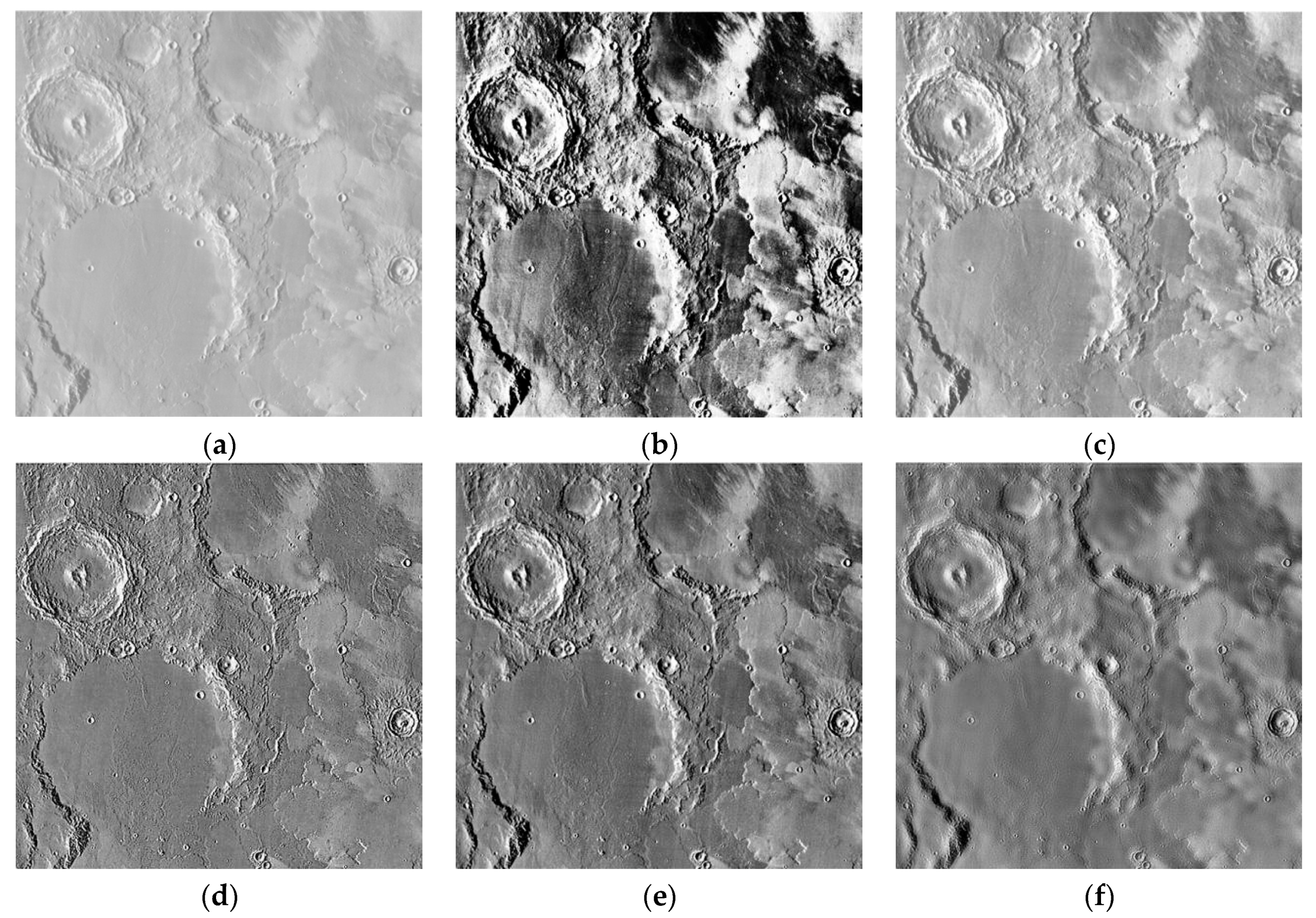
Figure 6 is the result of the five approaches simulated on Image 2. The size of the original remote sensing image is 548 × 548. Figure 6a depicts the original image; Figure 6b is the image enhanced using the HE technique, and also displays the over-enhancement phenomenon in some regions; Figure 6c is the enhanced result obtained by the ESIHE method; Figure 6d is the result achieved by FLM; the result obtained by LSCN is shown in Figure 6e; the enhanced result achieved by the proposed algorithm is shown in Figure 6f. From the enhancement results, we can see that the proposed method has achieved the goal of noise suppression and image details preserving.
Figure 7 is the enhanced result of the five image enhancement methods simulated on Image 3. The size of the original image is 256 × 256. Figure 7a is the original remote sensing image; Figure 7b,c are the enhanced results achieved by the HE and ESIHE approaches, respectively; the enhancement result obtained using the FLM approach is shown in Figure 7d, with an image transformation that is too light and severely distorted; Figure 7e depicts the result enhanced by the LSCN algorithm, which has achieved enhanced effects to some extent; Figure 7f presents the enhancement result obtained by the proposed method. From the results, we notice that the proposed approach has better performance due to the fact that it makes the enhanced image have moderate brightness, rich detail, and clear edges.
4.2. Objective Analysis
The Entropy (H) shows the overall information of the image, and it can be calculated by the following equation [15]:
where M × N represents the size of the image. A higher H shows that the image contains more effective information.
The Mean Square Error (MSE) is computed by:
The MSE shows the difference between the estimated image and the reference image [33]. A lower MSE demonstrates that the enhanced image is closer to the reference image.
The Peak Signal to Noise Ratio (PSNR) is computed by the following equation:
where L presents the maximum intensity in the image [38]. The higher the PSNR, the better the image quality.
The Gradient Magnitude Similarity Deviation (GMSD) reflects the range of distortion degree in the image; a higher GMSD reflects larger distortion and lower image quality, and can be calculated by [35]:
where N represents the number of pixels in the image, and GMSM is Gradient Magnitude Similarity Mean. A higher GMSM represents higher image quality, and it is defined as:
where GMS is gradient magnitude similarity, and the corresponding formula is described as follows:
where c is a positive constant, mr and md are the gradient magnitude images, and mr and md can be calculated by:
where ”⊗“ is the convolution operation.
The Mean Absolute Error (MAE) can be defined as:
where gx,y and fx,y denote the original image pixel and the enhanced image pixel, respectively [36]. If the MAE is lower, then the image quality is better.
The Multi-scale structural similarity (MSSSIM) is an improved evaluation metric based on structural similarity (SSIM). The higher the value of MSSSIM, the better the quality of the image. It is defined as [39]:
From Table 1, we notice that the H obtained by the proposed method is the best; for the metrics MSE, PSNR, MAE, and MSSSIM, the values achieved by the ESIHE method are the best, but the values obtained by the proposed algorithm in these four metrics are still second-best; for the index GMSD, the ESIHE method is the best, and the LSCN and proposed methods are second and third, respectively. From the data as shown in Table 2, the H, MSE, PSNR, and MAE values achieved by the proposed technique are the best; for the GMSD, the value achieved by the ESIHE method is the best, but the proposed approach is second; for the metric MSSSIM, the FLM method is the best, and the ESIHE and proposed techniques are the second and third, respectively. From Table 3, the H value achieved by the proposed method is the best; for the indicators of MSE, PSNR, MAE, and MSSSIM, the corresponding values achieved by the ESIHE method are the best, but values obtained by the proposed technique are still second-best in these metrics; for the indicator GMSD, the ESIHE method is the best, and the values achieved by the LSCN and proposed methods are second and third, respectively.
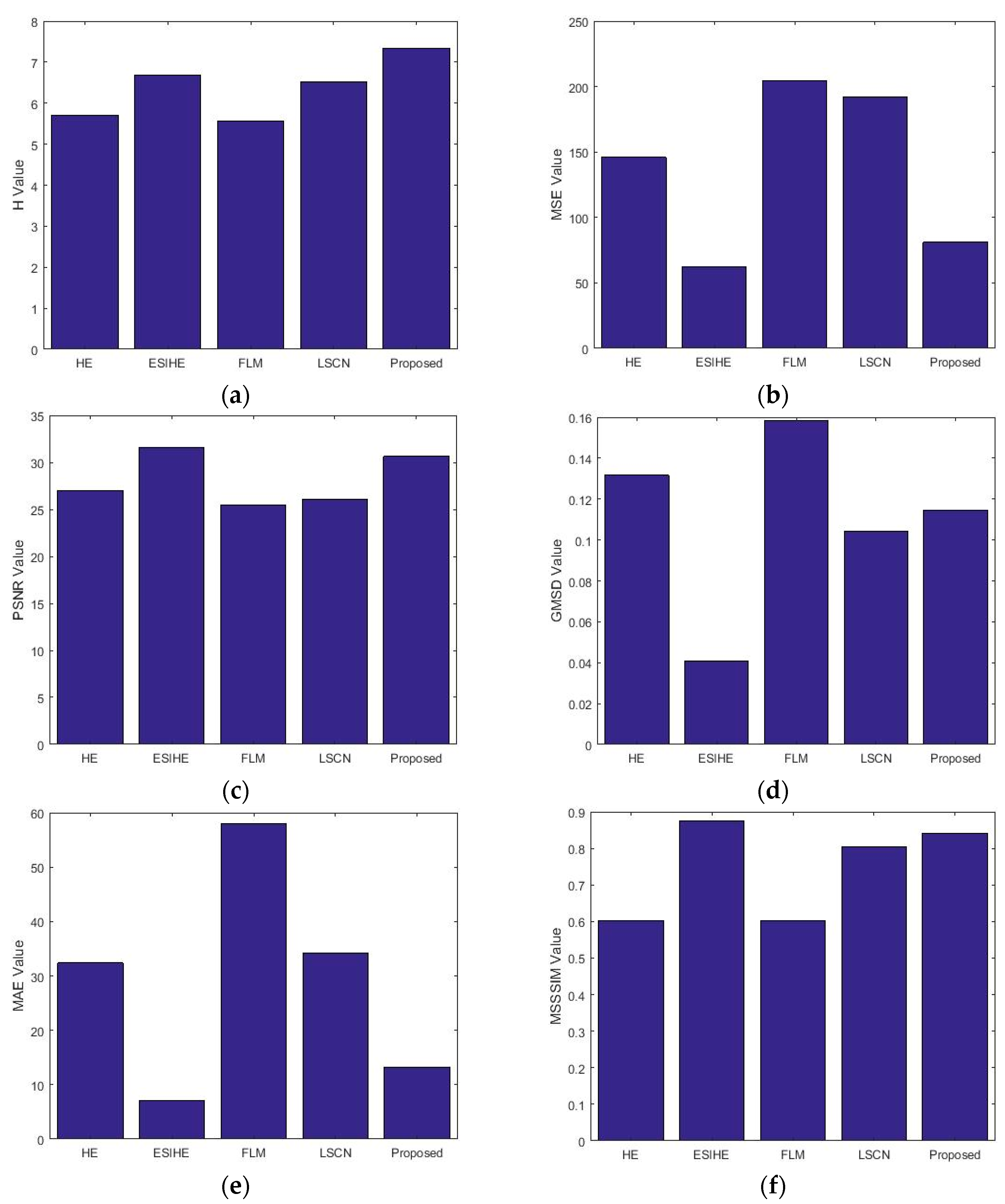
In order to demonstrate that the proposed technique has a better universality than the existing methods, we simulated 20 remote sensing images (as shown in Figure 8) and calculated the average values of the metrics (as shown in Table 4). Figure 9 depicts the histogram of the experimental data in Table 4. From these data, the proposed method shows advantages in terms of the six evaluation metrics when compared to other methods.
5. Conclusions
In this paper, a novel remote sensing image enhancement technique based on a non-local means filter in NSCT domain is proposed. This method was tested on different remote sensing images. After an image is decomposed by NSCT transform, there will be one low-frequency sub-band and several high-frequency sub-bands. Contrast stretching is applied to enhance the contrast of the low-frequency component, and the non-local means filter is used to suppress the noise contained in the first high-frequency sub-band. The processed coefficients are then reconstructed using the inverse nonsubsampled contourlet transform. Finally, the unsharp filter is adopted to enhance the details of the reconstructed image. The performance of the proposed method was evaluated and compared using the H, MSE, PSNR, GMSD, MAE, and MSSSIM metrics. Experimental results demonstrate that the proposed algorithm has better performance when compared with other existing techniques.
Acknowledgments
This work was supported by the Key Scientific and Technological Research Project of Jilin Province under Grant Nos. 20150204039GX and 20170414017GH; the Key Scientific and Technological Project of Changchun Government under Grant No. 14KG064; the Natural Science Foundation of Guangdong Province under Grant No. 2016A030313658; the Innovation and Strengthening School Project (provincial key platform and major scientific research project) supported by Guangdong Government under Grant No. 2015KTSCX175; the Premier-Discipline Enhancement Scheme Supported by Zhuhai Government and Premier Key-Discipline Enhancement Scheme Supported by Guangdong Government Funds.
Author Contributions
The experimental measurements and data collection were carried out by Liangliang Li and Yujuan Si. The manuscript was written by Liangliang Li with the assistance of Yujuan Si and Zhenhong Jia. All authors reviewed the manuscript.
Conflicts of Interest
The authors declare no conflicts of interest.
References
- Rahman, S.; Rahman, M.M.; Abdullah-Al-Wadud, M. An adaptive gamma correction for image enhancement. Eurasip J. Image Video Process. 2016, 2016, 35. [Google Scholar] [CrossRef]
- Asmatullah, C.; Kim, J. Improved adaptive fuzzy punctual kriging filter for image restoration. Int. J. Innov. Comput. Inf. Control 2013, 9, 583–598. [Google Scholar]
- Cao, G.; Zhao, Y.; Ni, R.; Li, X. Contrast enhancement-based forensics in digital images. IEEE Trans. Inf. Forensics Secur. 2014, 9, 515–525. [Google Scholar] [CrossRef]
- Panagiotakis, C.; Kokinou, E.; Sarris, A. Curvilinear structure enhancement and detection in geophysical images. IEEE Trans. Geosci. Remote Sens. 2011, 49, 2040–2048. [Google Scholar] [CrossRef]
- Bedi, S.; Khandelwal, R. Various image enhancement techniques—A critical review. Int. J. Adv. Res. Comput. Commun. Eng. 2013, 2, 1605–1609. [Google Scholar]
- Gao, G.; Wan, X.; Yao, S. Reversible data hiding with contrast enhancement and tamper localization for medical images. Inf. Sci. 2017, 385, 250–265. [Google Scholar] [CrossRef]
- Babu, P.; Rajamani, V. Contrast enhancement using real coded genetic algorithm based modified histogram equalization for gray scale images. Int. J. Imaging Syst. Technol. 2015, 25, 24–32. [Google Scholar] [CrossRef]
- Lisani, J.; Michel, J.; Morel, J.M. An inquiry on contrast enhancement methods for satellite images. IEEE Trans. Geosci. Remote Sens. 2016, 54, 7044–7054. [Google Scholar] [CrossRef]
- Schmitt, A. Multiscale and multidirectional multilooking for SAR image enhancement. IEEE Trans. Geosci. Remote Sens. 2016, 54, 5117–5134. [Google Scholar] [CrossRef]
- Pu, X.; Jia, Z.; Wang, L. The remote sensing image enhancement based on nonsubsampled contourlet transform and unsharp masking. Concurr. Comput. Pract. Exp. 2014, 26, 742–747. [Google Scholar] [CrossRef]
- Chang, Y.T.; Wang, J.T.; Yang, W.H. A novel contrast enhancement technique on palm bone images. Algorithms 2014, 7, 444–455. [Google Scholar] [CrossRef]
- Yu, C.Y.; Lin, H.Y.; Lin, R.N. Eight-scale image contrast enhancement based on adaptive inverse hyperbolic tangent algorithm. Algorithms 2014, 7, 98–102. [Google Scholar] [CrossRef]
- Chen, S.; Ramli, A.R. Minimum mean brightness error bi-histogram equalization in contrast enhancement. IEEE Trans. Consum. Electron. 2003, 49, 1310–1319. [Google Scholar] [CrossRef]
- Wang, Y.; Chen, Q.; Zhang, B. Image enhancement based on equal area dualistic sub-image histogram equalization method. IEEE Trans. Consum. Electron. 1999, 45, 68–75. [Google Scholar] [CrossRef]
- Singh, K.; Rajiv, K. Image enhancement using exposure based sub image histogram equalization. Pattern Recognit. Lett. 2014, 36, 10–14. [Google Scholar] [CrossRef]
- Xiao, Z.; Zhang, X. Diabetic retinopathy retinal image enhancement based on gamma correction. J. Med. Imaging Health Inform. 2017, 7, 149–154. [Google Scholar] [CrossRef]
- Huang, S.; Cheng, F.C.; Chiu, Y.S. Efficient contrast enhancement using adaptive gamma correction with weighting distribution. IEEE Trans. Image Process. 2013, 22, 1032–1041. [Google Scholar] [CrossRef] [PubMed]
- Kaur, A.; Singh, C. Contrast enhancement for cephalometric images using wavelet-based modified adaptive histogram equalization. Appl. Soft Comput. 2017, 51, 180–191. [Google Scholar] [CrossRef]
- Ansari, R.; Budhhiraju, K.M. A comparative evaluation of denoising of remotely sensed images using wavelet, curvelet and contourlet transforms. J. Indian Soc. Remote Sens. 2016, 44, 843–853. [Google Scholar] [CrossRef]
- Do, M.; Vetterli, M. The contourlet transform: an efficient directional multiresolution image representation. IEEE Trans. Image Process. 2005, 14, 2091–2106. [Google Scholar] [CrossRef] [PubMed]
- Cunha, A.; Zhou, J.; Do, M.N. The nonsubsampled contourlet transform: Theory, design, and applications. IEEE Trans. Image Process. 2006, 15, 3089–3101. [Google Scholar] [CrossRef] [PubMed]
- Li, Y.; Hu, J.; Jia, Y. Automatic SAR image enhancement based on nonsubsampled contourlet transform and memetic algorithm. Neurocomputing 2014, 134, 70–78. [Google Scholar] [CrossRef]
- Zhang, Q.; Maldague, X. Multisensor image fusion approach utilizing hybrid pre-enhancement and double nonsubsampled contourlet transform. J. Electron. Imaging. 2017, 26, 010501. [Google Scholar] [CrossRef]
- Zhou, F.; Jia, Z.; Yang, J. Method of improved fuzzy contrast combined adaptive threshold in NSCT for medical image enhancement. BioMed. Res. Int. 2017, 2017, 3969152. [Google Scholar] [CrossRef] [PubMed]
- Li, J. Optimal image-fusion method based on nonsubsampled contourlet transform. Opt. Eng. 2012, 51, 107006. [Google Scholar]
- Buades, A.; Coll, B.; Morel, J.M. A non-local algorithm for image denoising. In Proceedings of the IEEE Computer Society Conference on Computer Vision and Pattern Recognition, San Diego, CA, USA, 20–25 June 2005; pp. 60–65. [Google Scholar]
- Devapal, D.; Kumar, S.S.; Jojy, C. A novel approach of despeckling SAR images using nonlocal means filtering. J. Indian Soc. Remote Sens. 2017, 45, 443–450. [Google Scholar] [CrossRef]
- Lv, D.; Jia, Z.; Yang, J. Remote sensing image enhancement based on the combination of nonsubsampled shearlet transform and guided filtering. Opt. Eng. 2016, 55, 103104. [Google Scholar] [CrossRef]
- Hossain, F.; Alsharif, M. Minimum mean brightness error dynamic histogram equalization for brightness preserving image contrast enhancement. Int. J. Innov. Comput. Inf. Control 2009, 5, 3263–3274. [Google Scholar]
- Zhan, K.; Teng, J.; Shi, J. Feature-linking model for image enhancement. Neural Comput. 2016, 28, 1072–1100. [Google Scholar] [CrossRef] [PubMed]
- Zhan, K.; Shi, J.; Teng, J. Linking synaptic computation for image enhancement. Neurocomputing 2017, 238, 1–12. [Google Scholar] [CrossRef]
- Ayiguli, W.; Jia, Z.; Qin, X. Medical image enhancement based on shearlet transform and unsharp masking. J. Med. Imaging Health Inform. 2014, 4, 814–818. [Google Scholar]
- Elyasi, I.; Pourmina, M.A.; Moin, M.S. Speckle reduction in breast cancer ultrasound images by using homogeneity modified bayes shrink. Measurement 2016, 91, 55–65. [Google Scholar] [CrossRef]
- Liu, L.; Jia, Z.; Yang, J. A medical image enhancement method using adaptive thresholding in NSCT domain combined unsharp masking. Int. J. Imaging Syst. Technol. 2015, 25, 199–205. [Google Scholar] [CrossRef]
- Xue, W.; Zhang, L.; Mou, X. Gradient magnitude similarity deviation: A highly efficient perceptual image quality index. IEEE Trans. Image Process. 2014, 23, 684–695. [Google Scholar] [CrossRef] [PubMed]
- Choi, I.H.; Nam, Y.O.; Song, B.C. A content-adaptive sharpness enhancement algorithm using 2D FIR filters trained by pre-emphasis. J. Vis. Commun. Image Represent. 2013, 24, 579–591. [Google Scholar] [CrossRef]
- Fei, X.; Xiao, L.; Sun, Y.B. Perceptual image quality assessment based on structural similarity and visual masking. Signal Process. Image Commun. 2012, 27, 772–783. [Google Scholar] [CrossRef]
- Elyasi, I.; Pourmina, M.A. Reduction of speckle noise ultrasound images based on TV regularization and modified bayes shrink techniques. Opt. Int. J. Light Electron Opt. 2016, 127, 11732–11744. [Google Scholar] [CrossRef]
- Wang, Z.; Simoncelli, E.P.; Bovik, A.C. Multi-scale structural similarity for image quality assessment. In Proceedings of the IEEE Asilomar Conference on Signals, Systems and Computers, Pacific Grove, CA, USA, 9–12 November 2003; pp. 1398–1402. [Google Scholar]
Figure 1.
(a) The frequency model of nonsubsampled pyramid filter bank (NSPFB); (b) the frequency model of nonsubsampled directional filter bank (NSDFB); (c) the four-channel model of NSPFB.
Figure 1.
(a) The frequency model of nonsubsampled pyramid filter bank (NSPFB); (b) the frequency model of nonsubsampled directional filter bank (NSDFB); (c) the four-channel model of NSPFB.
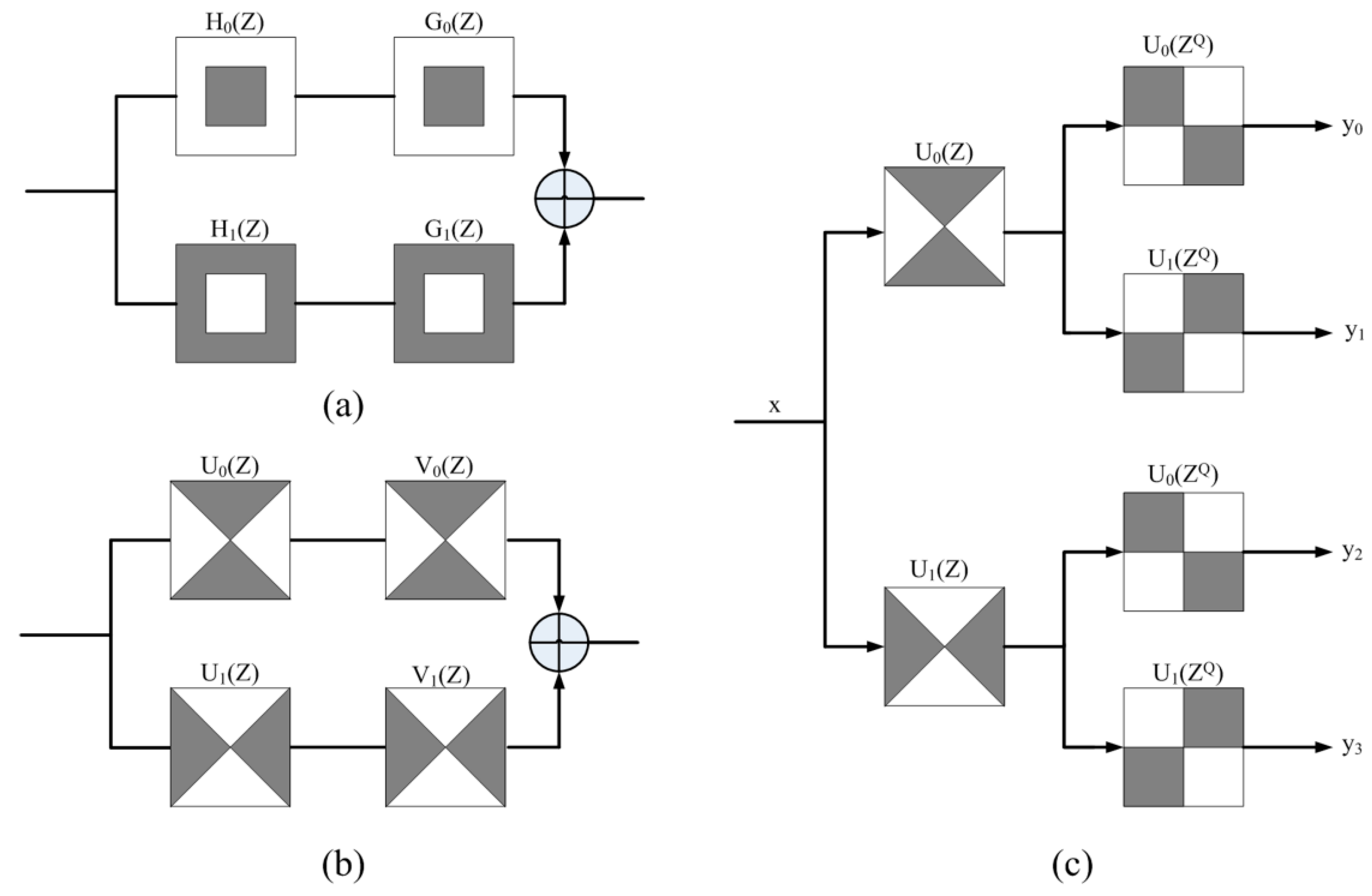
Figure 2.
The structure diagram of nonsubsampled contourlet transform (NSCT). (a) Non-subsampled filter bank model; (b) idealized frequency partitioning.
Figure 2.
The structure diagram of nonsubsampled contourlet transform (NSCT). (a) Non-subsampled filter bank model; (b) idealized frequency partitioning.
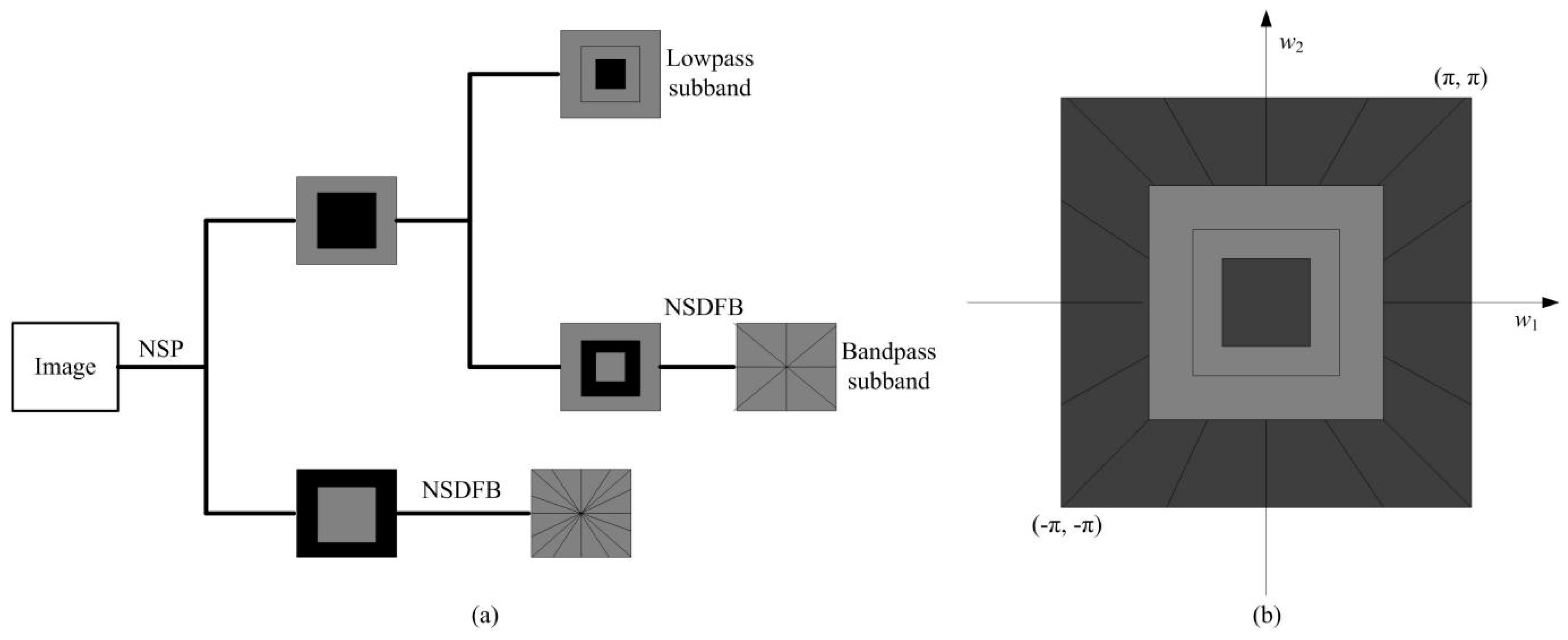
Figure 3.
Nonsubsampled contourlet transform (NSCT) decomposition of zoneplate image. (a) Zoneplate (256 × 256); (b) approximate NSCT coefficients; (c) detailed coefficients.
Figure 3.
Nonsubsampled contourlet transform (NSCT) decomposition of zoneplate image. (a) Zoneplate (256 × 256); (b) approximate NSCT coefficients; (c) detailed coefficients.
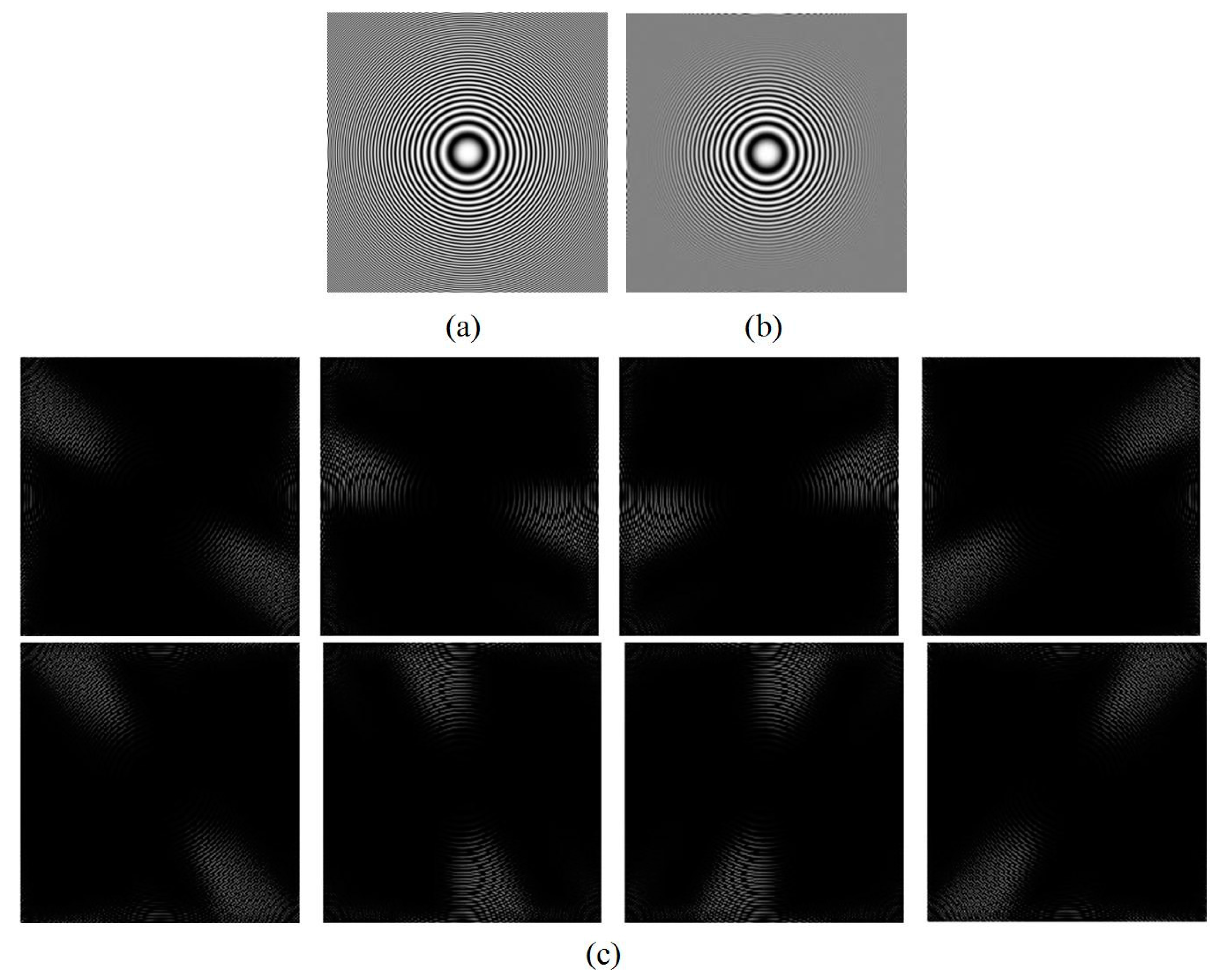
Figure 4.
The flow chart of the proposed method.
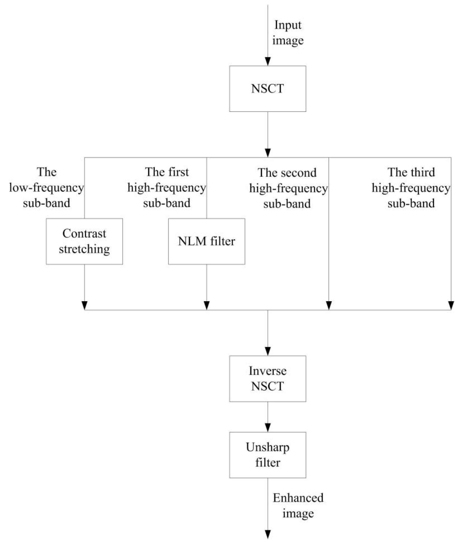
Figure 5.
Comparisons on Image 1. (a) Original image; (b) Histogram equalization (HE); (c) Exposure based sub-image histogram equalization (ESIHE); (d) Feature-linking model (FLM); (e) Linking synaptic computation (LSCN); (f) Proposed method.
Figure 5.
Comparisons on Image 1. (a) Original image; (b) Histogram equalization (HE); (c) Exposure based sub-image histogram equalization (ESIHE); (d) Feature-linking model (FLM); (e) Linking synaptic computation (LSCN); (f) Proposed method.

Figure 6.
Comparisons on Image 2. (a) Original image; (b) HE; (c) ESIHE; (d) FLM; (e) LSCN; (f) Proposed method.
Figure 6.
Comparisons on Image 2. (a) Original image; (b) HE; (c) ESIHE; (d) FLM; (e) LSCN; (f) Proposed method.

Figure 7.
Comparisons on Image 3. (a) Original image; (b) HE; (c) ESIHE; (d) FLM; (e) LSCN; (f) Proposed method.
Figure 7.
Comparisons on Image 3. (a) Original image; (b) HE; (c) ESIHE; (d) FLM; (e) LSCN; (f) Proposed method.
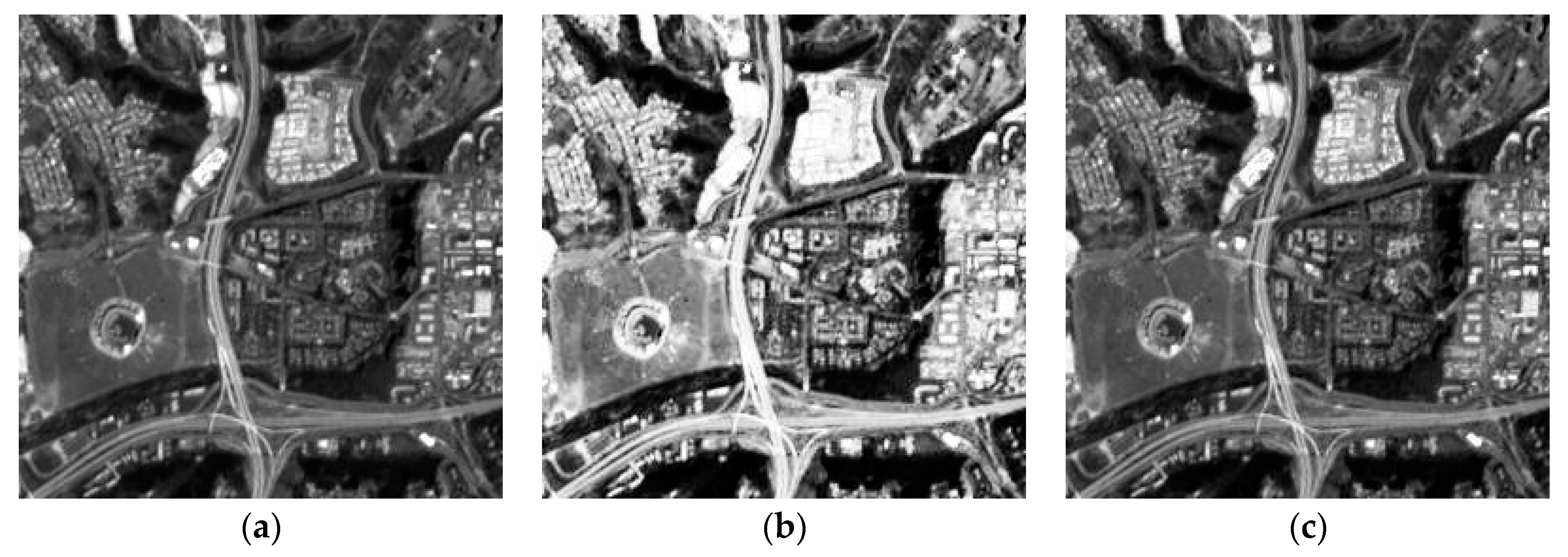
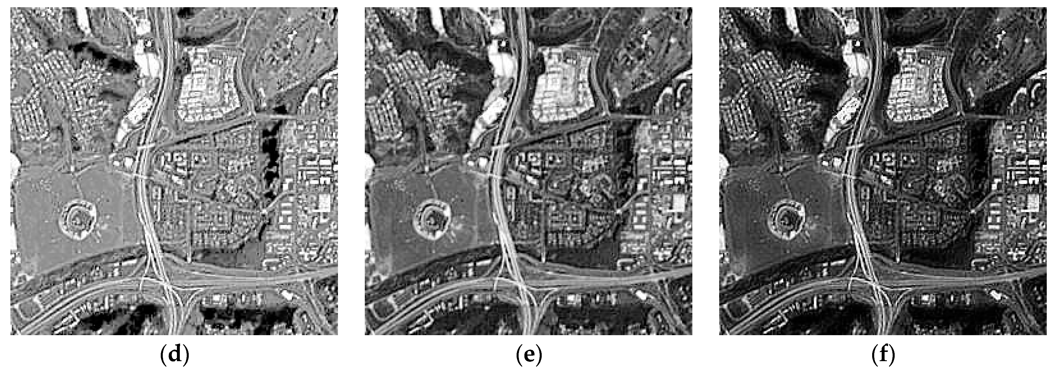
Figure 8.
The 20 images used for simulation with the five methods.
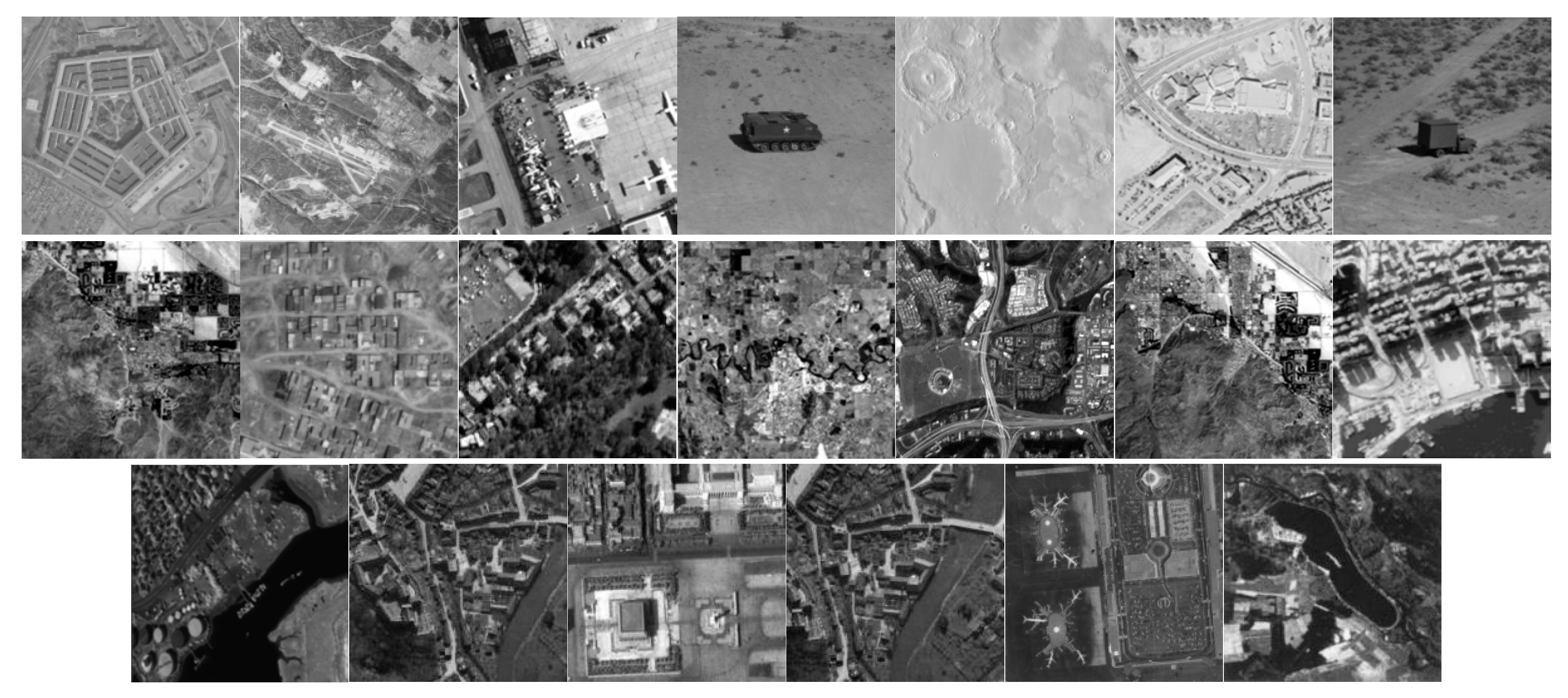
Figure 9.
The histogram of experimental data in Table 4. (a) H; (b) MSE; (c) PSNR; (d) GMSD; (e) MAE; (f) MSSSIM.
Figure 9.
The histogram of experimental data in Table 4. (a) H; (b) MSE; (c) PSNR; (d) GMSD; (e) MAE; (f) MSSSIM.

Table 1.
The evaluation metrics of the five methods on Image 1.
| HE | ESIHE | FLM | LSCN | Proposed | |
|---|---|---|---|---|---|
| H | 5.8139 | 7.3840 | 5.4117 | 6.9739 | 7.7279 |
| MSE | 109.5441 | 52.9798 | 157.0788 | 133.5418 | 61.4857 |
| PSNR | 27.7349 | 30.8897 | 26.1696 | 26.8746 | 30.2431 |
| GMSD | 0.0916 | 0.0220 | 0.1275 | 0.0653 | 0.0831 |
| MAE | 9.0398 | 4.4681 | 22.2944 | 13.1778 | 7.5462 |
| MSSSIM | 0.9433 | 0.9604 | 0.8789 | 0.9546 | 0.9560 |
H, entropy; MSE, mean square error; PSNR, peak signal to noise ratio; GMSD, gradient magnitude similarity deviation; MAE, mean absolute error; MSSSIM, multi-scale structural similarity.
Table 2.
The evaluation metrics of the five methods on Image 2.
| HE | ESIHE | FLM | LSCN | Proposed | |
|---|---|---|---|---|---|
| H | 5.3680 | 5.7781 | 4.7970 | 6.2201 | 6.9939 |
| MSE | 55.3809 | 23.1740 | 10.9848 | 2.9688 | 0.9760 |
| PSNR | 30.6972 | 34.4808 | 37.7229 | 43.4050 | 48.2362 |
| GMSD | 0.2172 | 0.0929 | 0.1680 | 0.1257 | 0.1161 |
| MAE | 6.4192 | 2.1371 | 1.3861 | 0.2497 | 0.0923 |
| MSSSIM | 0.1495 | 0.6382 | 0.6634 | 0.5354 | 0.6043 |
Table 3.
The evaluation metrics of the five methods on Image 3.
| HE | ESIHE | FLM | LSCN | Proposed | |
|---|---|---|---|---|---|
| H | 5.9682 | 7.3231 | 5.7467 | 7.1225 | 7.4585 |
| MSE | 186.9627 | 36.1431 | 226.8316 | 186.8378 | 49.5929 |
| PSNR | 25.4133 | 32.5506 | 24.5738 | 25.4162 | 31.1766 |
| GMSD | 0.1136 | 0.0074 | 0.1655 | 0.1058 | 0.1070 |
| MAE | 43.4997 | 4.1402 | 56.8070 | 24.3111 | 6.4677 |
| MSSSIM | 0.6896 | 0.9869 | 0.6189 | 0.9034 | 0.9269 |
Table 4.
The average evaluation metrics of the five methods on 20 remote sensing images.
| HE | ESIHE | FLM | LSCN | Proposed | |
|---|---|---|---|---|---|
| H | 5.7086 | 6.6722 | 5.5638 | 6.5150 | 7.3452 |
| MSE | 145.9162 | 62.2076 | 204.3192 | 192.4159 | 81.1120 |
| PSNR | 27.0276 | 31.6272 | 25.5021 | 26.0704 | 30.6440 |
| GMSD | 0.1317 | 0.0407 | 0.1586 | 0.1041 | 0.1145 |
| MAE | 32.3724 | 7.1230 | 58.0083 | 34.2755 | 13.2823 |
| MSSSIM | 0.6031 | 0.8760 | 0.6018 | 0.8037 | 0.8415 |
© 2017 by the authors. Licensee MDPI, Basel, Switzerland. This article is an open access article distributed under the terms and conditions of the Creative Commons Attribution (CC BY) license (http://creativecommons.org/licenses/by/4.0/).
Share and Cite
MDPI and ACS Style
Li, L.; Si, Y.; Jia, Z. Remote Sensing Image Enhancement Based on Non-Local Means Filter in NSCT Domain. Algorithms 2017, 10, 116. https://doi.org/10.3390/a10040116
AMA Style
Li L, Si Y, Jia Z. Remote Sensing Image Enhancement Based on Non-Local Means Filter in NSCT Domain. Algorithms. 2017; 10(4):116. https://doi.org/10.3390/a10040116
Chicago/Turabian StyleLi, Liangliang, Yujuan Si, and Zhenhong Jia. 2017. "Remote Sensing Image Enhancement Based on Non-Local Means Filter in NSCT Domain" Algorithms 10, no. 4: 116. https://doi.org/10.3390/a10040116
Note that from the first issue of 2016, this journal uses article numbers instead of page numbers. See further details here.