An Optimization Algorithm Inspired by the Phase Transition Phenomenon for Global Optimization Problems with Continuous Variables

1
School of Computer Science and Engineering, Xi’an University of Technology, Xi’an 710048, China
2
School of Computer Science and Engineering, Xi’an Technological University, Xi’an 710021, China
*
Author to whom correspondence should be addressed.
Algorithms 2017, 10(4), 119; https://doi.org/10.3390/a10040119
Submission received: 8 September 2017
/
Revised: 29 September 2017
/
Accepted: 9 October 2017
/
Published: 20 October 2017
Abstract
:In this paper, we propose a novel nature-inspired meta-heuristic algorithm for continuous global optimization, named the phase transition-based optimization algorithm (PTBO). It mimics three completely different kinds of motion characteristics of elements in three different phases, which are the unstable phase, the meta-stable phase, and the stable phase. Three corresponding operators, which are the stochastic operator of the unstable phase, the shrinkage operator in the meta-stable phase, and the vibration operator of the stable phase, are designed in the proposed algorithm. In PTBO, the three different phases of elements dynamically execute different search tasks according to their phase in each generation. It makes it such that PTBO not only has a wide range of exploration capabilities, but also has the ability to quickly exploit them. Numerical experiments are carried out on twenty-eight functions of the CEC 2013 benchmark suite. The simulation results demonstrate its better performance compared with that of other state-of-the-art optimization algorithms.
1. Introduction
Nature-inspired optimization algorithms have become of increasing interest to many researchers in optimization fields in recent years [1]. After half a century of development, nature-inspired optimization algorithms have formed a great family. It not only has a wide range of contact with biological, physical, and other basic science, but also involves many fields such as artificial intelligence, artificial life, and computer science.
Due to the differences in natural phenomena, these optimization algorithms can be roughly divided into three types. These are algorithms based on biological evolution, algorithms based on swarm behavior, and algorithms based on physical phenomena. Typical biological evolutionary algorithms are Evolutionary Strategies (ES) [2], Evolutionary Programming (EP) [3], the Genetic Algorithm (GA) [4,5,6], Genetic Programming (GP) [7], Differential Evolution (DE) [8], the Backtracking Search Algorithm (BSA) [9], Biogeography-Based Optimization (BBO) [10,11], and the Differential Search Algorithm (DSA) [12].
In the last decade, swarm intelligence, as a branch of intelligent computation models, has been gradually rising [13]. Swarm intelligence algorithms mainly simulate biological habits or behavior, including foraging behavior, search behavior and migratory behavior, brooding behavior, and mating behavior. Inspired by these phenomena, researchers have designed many intelligent algorithms, such as Ant Colony Optimization (ACO) [14], Particle Swarm Optimization (PSO) [15], Bacterial Foraging (BFA) [16], Artificial Bee Colony (ABC) [17,18,19], Group Search Optimization (GSO) [20], Cuckoo Search (CS) [21,22], Seeker Optimization (SOA) [23], the Bat Algorithm (BA) [24], Bird Mating Optimization (BMO) [25], Brain Storm Optimization [26,27] and the Grey Wolf Optimizer (GWO) [28].
In recent years, in addition to the above two kinds of algorithms, intelligent algorithms simulating physical phenomenon have also attracted a great deal of researchers’ attention, such as the Gravitational Search Algorithm (GSA) [29], the Harmony Search Algorithm (HSA) [30], the Water Cycle Algorithm (WCA) [31], the Intelligent Water Drops Algorithm (IWDA) [32], Water Wave Optimization (WWO) [33], and States of Matter Search (SMS) [34]. The classical optimization algorithm about a physical phenomenon is simulated annealing, which is based on the annealing process of metal [35,36].
Though these meta-heuristic algorithms that have many advantages over traditional algorithms, especially in NP hard problems, have been proposed to tackle many challenging complex optimization problems in science and industry, there is no single approach that is optimal for all optimization problems [37]. In other words, an approach may be suitable for solving these problems, but it is not suitable for solving those problems. This is especially true as global optimization problems have become more and more complex, from simple uni-modal functions to hybrid rotated shifted multimodal functions [38]. Hence, more innovative and effective optimization algorithms are always needed.
A natural phenomenon provides a rich source of inspiration to researchers to develop a diverse range of optimization algorithms with different degrees of usefulness and practicability. In this paper, a new meta-heuristic optimization algorithm inspired by the phase transition phenomenon of elements in a natural system for continuous global optimization is proposed, which is termed phase transition-based optimization (PTBO). From a statistical mechanics point of view, a phase transition is a non-trivial macroscopic form of collective behavior in a system composed of a number of elements that follow simple microscopic laws [39]. Phase transitions play an important role in the probabilistic analysis of combinatorial optimization problems, and are successfully applied in Random Graph, Satisfiability, and Traveling Salesman Problems [40]. However, there are few algorithms with the mechanism of phase transition for solving continuous global optimization problems in the literature.
Phase transition is ubiquitous in nature or in social life. For example, at atmospheric pressure, water boils at a critical temperature of 100 °C. When the temperature is lower than 100 °C, water is a liquid, while above 100 °C, it is a gas. Besides this, there are also a lot of examples of phase transition. Everybody knows that magnets attract nails made out of iron. However, the attraction force disappears when the temperature of the nail is raised above 770 °C. When the temperature is above 770 °C, the nail enters a paramagnetic phase. Moreover, it is well-known that mercury is a good conductor for its weak resistance. Nevertheless, the electrical resistance of mercury falls abruptly down to zero when the temperature passes through 4.2 K (kelvin temperature). From a macroscopical view, a phase transition is the transformation of a system from one phase to another one, depending on the values of control parameters, such as temperature, pressure, and other outside interference.
From the above examples, we can see that each system or matter has different phases and related critical points for those phases. We can also observe that all phase transitions have a common law, and we may think that phase transition is the competitive result of two kinds of tendencies: stable order and unstable disorder. In complex system theory, phase transition is related to the self-organized process by which a system transforms from disorder to order. From this point of view, phase transition implicates a search process of optimization. The thermal motion of an element is a source of disorder [41]. The interaction of elements is the cause of order.
In the proposed PTBO algorithm, the degree of order or disorder is described by stability. We used the value of an objective function to depict the level of stability. For the sake of generality, we extract three kinds of phases in the process of transition from disorder to order, i.e., an unstable phase, a meta-stable phase [42] and a stable phase. From a microscopic viewpoint, the diverse motion characteristics of elements in different phases provide us with novel inspiration to develop a new meta-heuristic algorithm for solving complex continuous optimization problems.
This paper is organized as follows. In Section 2, we briefly introduce the prerequisite preparation for the phase transition-based optimization algorithm. In Section 3, the phase transition-based optimization algorithm and its operators are described. An analysis of PTBO and a comparative study are presented in Section 4. In Section 5, the experimental results with those of other state-of-the-art algorithms are demonstrated. Finally, Section 6 draws conclusions.
2. Prerequisite Preparation
2.1. Fundamental Concepts
Nature itself is a large complex system. In a natural system, the motion of elements transforming from an unstable phase (disorder) to a stable phase (order) is an eternal natural law. In this paper, we uniformly call a molecule in water, an atom in iron, an electron in mercury, etc., an element. The phase of an element in a system may be divided into an unstable phase, a meta-stable phase, and a stable phase. Figure 1 shows three possible positions of elements in a system.
From Figure 1, we can observe that an element is most unstable in the position of point A, and we intuitively call it an unstable phase. On the contrary, in the position of point C, the element is most stable, and we name it a stable phase. The position of point B, between point A and point C, is the transition phase, and we term it a meta-stable phase. The definitions of the three phases are as follows.
Definition 1.
Unstable Phase (UP). The element is in a phase of complete disorder, and moves freely towards an arbitrary direction. In the case of this phase, the element has a large range of motion, and has the ability of global divergence.
Definition 2.
Meta-stable Phase (MP). The element is in a phase between disorder and order, and moves according to a certain law, such as towards the lowest point. In the case of this phase, the element has a moderate activity, and possesses the ability of local shrinkage.
Definition 3.
Stable Phase (SP). The element is in a very regular phase of orderly motion. In the case of this phase, the element has a very small range of activity and has the ability of fine tuning.
According to the above definitions, we can give a more detailed description and examples about the characteristics of the three phases. These motion characteristics in three phases provide us with rich potential to develop the proposed PTBO algorithm. The following Table 1 summarizes the motional characteristics of the unstable phase, the meta-stable phase, and the stable phase.
2.2. The Determination of Critical Interval about Three Phases
As mentioned before, we use stability, which is depicted by the fitness value of an objective function, to describe the degree of order or disorder of an element. In our proposed algorithm, the higher the fitness value of an element is, the worse the stability is. The question of how to divide the critical intervals of the unstable phase, the meta-stable phase, and the stable phase is a primary problem that must be addressed before the proposed algorithm is designed.
For simplicity, we use to denote a maximum fitness value, and we say this element is in the most unstable phase. On the contrary, denotes a minimum fitness value. Then, we set up that the stable phase accounts for , and the proportion of the meta-stable phase is . So, the proportion of the unstable phase is . The ratio of three critical intervals is shown in Figure 2.
Although and are dynamically changed in each generation, which means the iteration process of phase transition, the basic relationship between the phase of the elements and the critical intervals is shown in Table 2.
3. Phase Transition-Based Optimization Algorithm
3.1. Basic Idea of the PTBO Algorithm
In this work, the motion of elements from an unstable phase to another relative stable phase in PTBO is as natural selection in GA. Many of these iterations from an unstable phase to another relative stable phase can eventually make an element reach absolute stability. The diverse motional characteristics of elements in the three phases are the core of the PTBO algorithm to simulate this phase transition process of elements. In the PTBO algorithm, three corresponding operators are designed. An appropriate combination of the three operators makes an effective search for the global minimum in the solution space.
3.2. The Correspondence of PTBO and the Phase Transition Process
Based on the basic law of elements transitioning from an unstable phase (disorder) to a stable phase (order), the correspondence of PTBO and phase transition can be summarized in Table 3.
3.3. The Overall Design of the PTBO Algorithm
The simplified cyclic diagram of the phase transition process in our PTBO algorithm is shown in Figure 3. It is a complete cyclic process of phase transition from an unstable phase to a stable phase. Firstly, in the first generation, we calculate the maximum and minimum fitness value for each element, respectively, and divide the critical intervals of the unstable phase, the meta-stable phase, and the stable phase according to the rules in Table 2. Secondly, the element will perform the relevant search according to its own phase. If the result of the new degree of stability is better than that of the original phase, the motion will be reserved. Otherwise, we will abandon this operation. That is to say, if the original phase of an element is UP, the movement direction may be towards UP, MP, and SP. However, if the original phase of an element is MP, the movement direction may be towards MP and SP. Of course, if the original phase of an element is SP, the movement direction is towards only SP. Finally, after much iteration, elements will eventually obtain an absolute stability.
Broadly speaking, we may think of PTBO as an algorithmic framework. We simply define the general operations of the whole algorithm about the motion of elements in the phase transition. In a word, PTBO is flexible for skilled users to customize it according to a specific scene of phase transition.
According to the above complete cyclic process of the phase transition, the whole operating process of PTBO can be summarized as three procedures: population initialization, iterations of three operators, and individual selection. The three operators in the iterations include the stochastic operator, the shrinkage operator, and the vibration operator.
3.3.1. Population Initialization
PTBO is also a population-based meta-heuristic algorithm. Like other evolutionary algorithms (EAs), PTBO starts with an initialization of a population, which contains a population size (the size is ) of element individuals. The current generation evolves into the next generation through the three operators described as below (see Section 3.3.2). That is to say, the population continually evolves along with the proceeding generation until the termination condition is met. Here, we initialize the j-th dimensional component of the i-th individual as
where is an uniformly distributed random number between 0 and 1, and are the upper boundary and lower boundary of j-th dimension of each individual, respectively.
3.3.2. Iterations of the Three Operators
Now we simply give some certain implementation details about the three operators in the three different phases.
(1) Stochastic operator
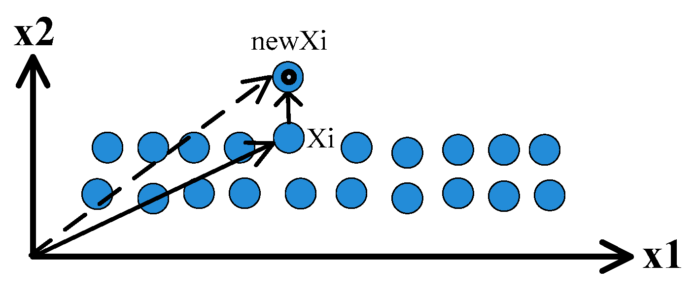
Stochastic diffusion is a common operation in which elements randomly move and pass one another in an unstable phase. Although the movement of elements is chaotic, it actually obeys a certain law from a statistical point of view. We can use the mean free path [43], which is a distance between an element and two other elements in two successive collisions, to represent the stochastic motion characteristic of elements in an unstable phase. Figure 4 simply shows the process of the free walking path of elements.
The free walking path of elements is the distance traveled by an element and other individuals through two collisions. Therefore, the stochastic operator of elements may be implemented as follows:
where is the new position of after the stochastic motion, and are two random vectors, where each element is a random number in the range (0, 1), and the indices j and k are mutually exclusive integers randomly chosen from the range between 1 and N that is also different from the indices i.
(2) Shrinkage operator
In a meta-stable phase, an element will be inclined to move closer to the optimal one. From a statistical standpoint, the geometric center is a very important digital characteristic and represents the shrinkage trend of elements in a certain degree. Figure 5 briefly gives the shrinkage trend of elements towards the optimal point.
Hence, the gradual shrinkage to the central position is the best motion to elements in a meta-stable phase. So, the shrinkage operator of elements may be implemented as follows:
where is the new position of after the shrinkage operation, is the best individual in the population, and is a normal random number with mean 0 and standard deviation 1. The Normal distribution is an important family of continuous probability distributions applied in many fields.
(3) Vibration operator
Elements in a stable phase will be apt to only vibrate about their equilibrium positions. Figure 6 briefly shows the vibration of elements.
Hence, the vibration operator of elements may be implemented as follows:
where is the new position of after the vibration operation, is a uniformly distributed random number in the range (0, 1), and is the control parameter which regulates the amplitude of jitter with a process of evolutionary generation. With the evolution of the phase transition, the amplitude of vibration will gradually become smaller. is described as follows:
where the and denote the maximum number of iterations and current number of iteration respectively, and stands for the exponential function.
3.3.3. Individual Selection
In the PTBO algorithm, like other EAs, one-to-one greedy selection is employed by comparing a parent individual and its new generated corresponding offspring. In addition, this greedy selection strategy may raise diversity compared with other strategies, such as tournament selection and rank-based selection. The selection operation at the k-th generation is described as follows:
where is the objective function value of each individual.
3.4. Flowchart and Implementation Steps of PTBO
As described above, the main flowchart of the PTBO algorithm is given in Figure 7.
The implementation steps of PTBO are summarized as follows:
Step 1. Initialization: set up algorithm parameters N, D, alpha and beta, randomly generate initial population of elements, and set ;
Step 2. Evaluation and partition interval: calculate the fitness values of all individuals and obtain the and , and divide the critical interval of UP, MP and SP according to Table 2;
Step 3. Stochastic operator: using Formula (2) to create ;
Step 4. Shrinkage operator: using Formula (3) to update ;
Step 5. Vibration operator: using Formula (4) and (5) to update ;
Step 6. Individual selection: accept if is better than ;
Step 7. Termination judgment: if termination condition is satisfied, stop the algorithm; otherwise, , go to Step 3.
4. The Analysis of PTBO and a Comparative Study
4.1. The Analysis of Time Complexity
For PTBO, the main operations include the operation of population initialization and the stochastic operator, shrinkage operator, and vibration operator. The time complexity of each operation in a single iteration can be computed as follows:
- 1
- Population initialization operation: .
- 2
- Stochastic operator: .
- 3
- Shrinkage operator: .
- 4
- Vibration operator: .
Therefore, the total worst time complexity of PTBO in one iteration is . According to the operational rules of the symbol O, the worst time complexity of one iteration for PTBO can be simplified as . It is worth noting that PTBO has the similar time complexity to some popular meta-heuristic algorithms such as PSO ().
4.2. The Dynamic Implementation Analysis of PTBO
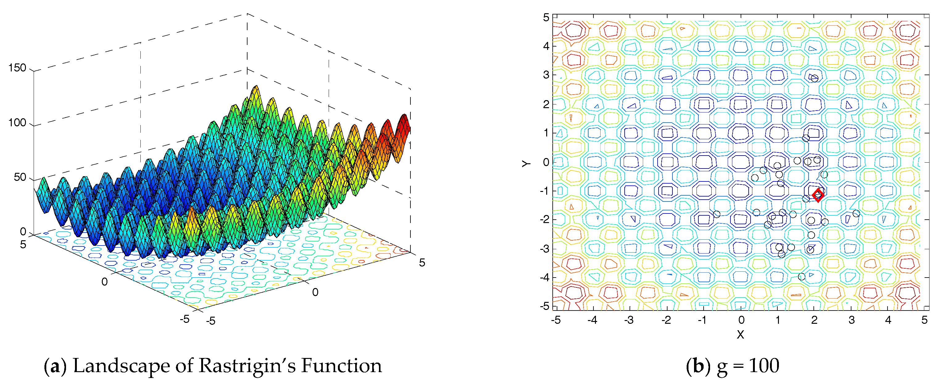
In this section, the step-wise procedure for the implementation of PTBO for optimization is presented. For the demonstration of the process, Rastrigin’s function [44] is herein considered as an example. Rastrigin’s function is a classic test function in optimization theory in which the point of global minimum is surrounded by a large number of local minima. To converge to the global minimum without being stuck at one of these local minima, however, is extremely difficult. Some numerical solvers need to take a long time to converge to it. Three-dimensional contour plot for Rastrigin’s function is shown in Figure 8a. Rastrigin’s function is described as follows:
In this experiment, we use 30 individuals to solve the above minimization problem, and the population distribution at various generations in an evolutionary process is shown in Figure 8b–f, with D = 2, alpha = 0.1 and beta = 0.8. In Figure 8b–f, the labels of red diamond represent the optimal point.
From Figure 8b–f, we can observe that the population distribution information can significantly vary at various generations during the run time. PTBO can effectively adapt to a time-varying search space or landscapes.
4.3. The Differences between PTBO and Other Algorithms
4.3.1. The Differences between PTBO and PSO
Like PSO (Particle Swarm Optimization), PTBO is also introduced to deal with unconstrained global optimization problems with continuous variables. In the representational form of implementation, we can certainly think that PTBO is also based on a particle system in the same way as PSO. However, according to the overall design of the PTBO algorithm, there are some differences between PTBO and the classical PSO.
Firstly, in heuristic thought, PSO is inspired by biological behavior or habits for simulating animal swarm behavior, such as fish schooling and bird flocking, while PTBO is inspired by the phase transition phenomenon of elements in nature. Secondly, in PSO, the direction of a particle is calculated by two best positions, and . However, the motion direction of an element in PTBO is arbitrarily derived from the other two elements that are different from each other. It may enhance the diversity of the population and ensure the avoidance of premature convergence. Thirdly, in the design of the operators, each particle in PSO contains a velocity item. Nevertheless, in PTBO the concept of velocity does not exist. Besides, PSO uses the position information of and to record the updating of velocity or position. However, PTBO uses only the position information about and the position of elements is not considered.
4.3.2. The Differences between PTBO and SMS
SMS (States of Matter Search) is a nature-inspired optimization algorithm based on the simulation of the states of matter phenomenon [35]. Specifically, SMS is devised by considering each state of matter at one different exploration–exploitation ratio by dividing the whole search process into three stages, i.e., gas, liquid, and solid.
Although the sources of inspiration for PBTO and SMS are similar, which are taken from a physical phenomenon about the states of matter, the evolution processes of PTBO and SMS are completely different. The evolution process of SMS is as follows. At first, all individuals in the population perform exploration in the mode of the gas state. Then, after 50% of the iterations, the search mode is changed into the liquid state for 40% of the iterations, i.e., the search between exploration and exploitation. Finally, the evolutionary process enters the stage of exploitation (liquid state) for 10% of the iterations. However, in PTBO, the three phases are coexistent in the entire search process. In other words, the three different phases of individuals execute dynamically different search tasks according to their phase in each generation. Hence, the implementation about the balance of exploration and exploitation between PTBO and SMS is completely different. Besides, the operators of PTBO and SMS are also completely different. In summary, it can be said that there are fundamental differences between PTBO and SMS.
5. Experimental Results
5.1. Benchmark Functions
In order to verify the effectiveness and robustness of the proposed PTBO algorithm, PTBO is applied in experimental simulation studies for finding the global minimum of the entire 28 test functions of the CEC 2013 special session [44]. The CEC 2013’s test suite, which has been improved on the basis of CEC 2005 [38], covers various types of function optimization, and is summarized in Table 4.
The search range of all functions is between −100 and 100 in every dimension. These problems are shifted or rotated to increase their complexity, and are treated as black-box problems. The explicit equations of the problems are not allowed to be used. The test suite of Table 4 consists of five uni-modal functions (F01 to F05), 15 multimodal functions (F06 to F20) and eight composition functions (F21 to F28).
5.2. Parameters Determination of the Interval Ratio of PTBO
In our PTBO algorithm, there are two parameters, the alpha and the beta, that need to be allocated to determine the critical intervals about the three phases. In a natural system, we can observe that the elements in the middle meta-stable phase account for the majority, and the elements in the unstable and stable phases occupy only a small proportion. This phenomenon is consistent with the two-eight law (or the 1/5th rule) [2]. For the case of simplicity, we give a value of 0.8 to beta, which is the proportion of the elements in the meta-stable phase. So, the elements in the unstable and stable phases account for 0.2 in total. The specific interval ratio settings of the three phases are shown in Table 5.
In order to determine which interval ratio is the most suitable for the PTBO algorithm, we conducted some compared experiments with 50 independent runs according to Table 5. The compared results of different interval ratios are listed in Table 6. In Table 6, the mean values are listed in the first line, and the standard deviations are displayed in the second line. We can intuitively observe that the ratio of prop4 has the best accuracy results compared with the other three ratios. Hence, in the subsequent experiments, we choose the value of beta to be 0.8, and the proportion of the unstable and stable phases is a random ratio of 0.2 in total.
5.3. Experimental Platform and Algorithms’ Parameter Settings
For a fair comparison, all of the experiments are conducted on the same machine with an Intel 3.4 GHz central processing unit (CPU) and 4GB memory. The operating system is Windows 7 with MATLAB 8.0.0.783(R2012b).
On the test functions, we compare PTBO with classic PSO, DE, and six other recent popular meta-heuristic algorithms, which are BA, CS, BSO, WWO, WCA, and SMS. The first three algorithms belong to the second category, i.e., swarm intelligence, and the remaining three algorithms belong to the third category, i.e., intelligent algorithms simulating physical phenomena. The parameters adopted for the PTBO algorithm and the compared algorithms are given in Table 7.
5.4. The Compared Experimental Results
Each of the experiments was repeated for 50 independent runs with different random seeds, and the average function values of the best solutions were recorded.
5.4.1. Comparisons on Solution Accuracy
The accuracy results of the uni-modal, multimodal, and composition functions are given in Table 8, Table 9 and Table 10, respectively. The accuracy results are in terms of the mean optimum solution and the standard deviation of the solutions obtained by each algorithm over 300,000 function evaluation times (FES) or 10,000 maximum generations. In all experiments, the dimensions of all problems are 30. The best results among the algorithms are shown in bold. In each row of the three tables, the mean values are listed in the first line, and the standard deviations are displayed in the second line. A two-tailed t-test [45] is performed with a 0.05 significance level to evaluate whether the median fitness values of two sets of obtained results are statistically different from each other. In the below three tables, if PTBO significantly outperforms another algorithm, a ‘ǂ’ is labeled in the back of the corresponding result obtained by this algorithm. Corresponding to ‘ξ’, ‘ξ’ denotes that PTBO is worse than other algorithms, and ‘~’ denotes that there is no significance between PTBO and the compared algorithm. At the last row of each table, a summary of the total number of ‘ǂ’, ‘ξ’, and ‘~’ is calculated.
(1) The accuracy results of uni-modal functions
The results of the uni-modal functions are shown in Table 8 in terms of the mean optimum solution and the standard deviation of the solutions.
In Table 8, among the five functions, PTBO has yielded the best results on two of them (F03 and F05). Although PTBO is worse than WCA, which obtains the best results on F01, F02, and F04, we observe from the statistical results that the performance of PTBO in uni-modal functions is significantly better than PSO, DE, BA, CS, BSO, WWO, and SMS.
(2) The accuracy results of multimodal functions
From Table 9, it can be observed that the mean value and the standard deviation value of PSO displays the best results for the function F15. DE obtains the best results on F07, F09, and F12, and BA has the best result for the function F06. BSO has the best result for the function F16. WCA obtains the best results on F8 and F10. CS, WWO, and SMS do not obtain any best result except for the function F8. With regard to the function F8, there is no big difference about all eight algorithms. The PTBO algorithm performs well for the functions F11, F13, F14, F17, F18, and F20, and according to the data of the last row in Table 9, it can be concluded that the PTBO algorithm has good performance in solution accuracy for multimodal benchmark functions.
(3) The accuracy results of composition functions
It can be seen from Table 10 that DE acquires the best results on F25, and WWO obtains the best results on F26. However, PTBO obtains the best results on F21, F22, F23, F24, F27, and F28. In general, PTBO shows the best overall performance from the statistical results according to the data of the last row in Table 10.
(4) The total results of solution accuracy of the 28 functions
5.4.2. The Comparison Results of Convergence Speed
Due to page limitation, Figure 9 presents the convergence graphs of parts of the 28 test functions in terms of the mean fitness values achieved by each of the nine algorithms for 50 runs. From Figure 9, it can be observed that PTBO converges towards the optimal values faster than the other algorithms in most cases, i.e., F1, F6, F12, F18, F21, F27, and F28.
5.4.3. The Comparison Results of Wilcoxon Signed-Rank Test
To further statistically compare PTBO with the other eight algorithms, a Wilcoxon signed-rank test [45] has been carried out to show the differences between PTBO and the other algorithms. The p-values on every function by a two-tailed test with a significance level of 0.05 between PTBO and other algorithms are given in Table 12.
From the results of the signed-rank test in Table 12, we can observe that our PTBO algorithm has a significant advantage over seven other algorithms in p-value, which are PSO, BA, CS, BSO, WWO, WCA, and SMS. Although PTBO has no significant advantage over DE, PTBO significantly outperforms DE in R+ value. R+ is the sum of ranks for the functions on which the first algorithm outperformed the second [46], and the differences are ranked according to their absolute values. So, according to the statistical results, it can be concluded that PTBO generally offered better performance than other algorithms for all 28 functions.
The above comparisons between PTBO and other nature-based meta-heuristic algorithms may offer a possible explanation for why PTBO could obtain better results on some optimization problems and that it is possible for PTBO to deal with more complex problems better.
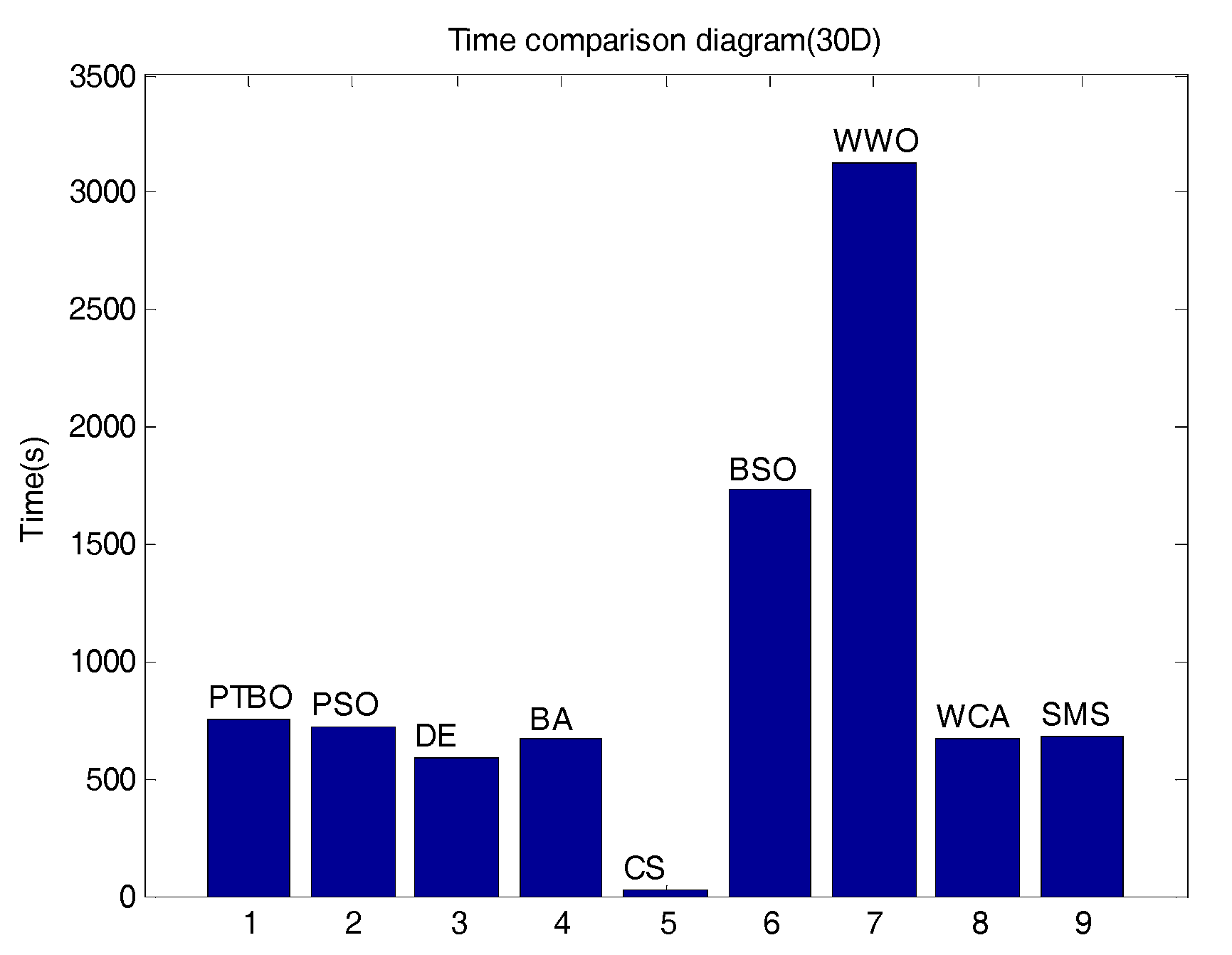
5.4.4. The Comparison Results of Time Complexity
The total comparisons of mean time complexity of the 28 functions about the nine algorithms are given in Figure 10. From Figure 10, we can observe that PTBO is ranked sixth, and is only better than BSO and WWO. However, we can find that the mean CPU time of PTBO is slightly worse than PSO and DE, and it also confirms the analysis in Section 4.1.
6. Conclusions
In this work, a new meta-heuristic optimization algorithm simulating the phase transition of elements in a natural system, named PTBO, has been described. Although the proposed PTBO algorithm is an algorithm with some similarities to the SMS and PSO algorithms, the main concepts are slightly different. It is very simple and very flexible when compared to the existing nature-inspired algorithms. It is also very robust, at least for the test problems considered in this work. From the numerical simulation results and comparisons, it is concluded that PTBO can be used for solving uni-modal and multimodal numerical optimization problems, and is similarly effective and efficient compared with other optimization algorithms. It is worth noting that PTBO performs slightly worse than PSO and DE in time complexity. In the future, further research contents include (1) developing a more effective division method for the three phases, (2) combining the PTBO algorithm with other evolution algorithms, and (3) applying PTBO to real-world optimization problems, such as the reliability–redundancy allocation problem and structural engineering design optimization problems.
Acknowledgments
This research was partially supported by Industrial Science and technology project of Shaanxi Science and Technology Department (Grant No. 2016GY-088) and the Project of Department of Education Science Research of Shaanxi Province (Grant No. 17JK0371). Besides those, this research was partially supported by the fund of National Laboratory of Network and Detection Control (Grant No. GSYSJ2016007). The author declares that the above funding does not lead to any conflict of interests regarding the publication of this manuscript.
Author Contributions
Lei Wang conceived and designed the framework; Zijian Cao performed the experiments and wrote the paper.
Conflicts of Interest
The author declares that there is no conflict of interests regarding the publication of this paper.
References
- Yang, X.S. Nature-Inspired Optimization Algorithms; Elsevier: Amsterdam, The Netherlands, 2014. [Google Scholar]
- Beyer, H.G.; Schwefel, H.P. Evolution strategies—A comprehensive introduction. Nat. Comput. 2002, 1, 3–52. [Google Scholar] [CrossRef]
- Fogel, L.J.; Owens, A.J.; Walsh, M.J. Artificial Intelligence through Simulated Evolution; Wiley: New York, NY, USA, 1966. [Google Scholar]
- Holland, J.H. Adaptation in Natural and Artificial Systems; University of Michigan Press, The MIT Press: London, UK, 1975. [Google Scholar]
- Garg, H. A hybrid PSO-GA algorithm for constrained optimization problems. Appl. Math. Comput. 2016, 274, 292–305. [Google Scholar] [CrossRef]
- Garg, H. A hybrid GA-GSA algorithm for optimizing the performance of an industrial system by utilizing uncertain data. In Handbook of Research on Artificial Intelligence Techniques and Algorithms; IGI Global: Hershey, PA, USA, 2015; pp. 620–654. [Google Scholar]
- Holland, J.R. Genetic Programming: On the Programming of Computers by Means of Natural Selection; MIT Press: London, UK, 1992. [Google Scholar]
- Storn, R.; Price, K. Differential evolution—A simple and efficient heuristic strategy for global optimization over continuous spaces. J. Glob. Optim. 1997, 11, 341–359. [Google Scholar] [CrossRef]
- Civicioglu, P. Backtracking search optimization algorithm for numerical optimization problems. Appl. Math. Comput. 2013, 219, 8121–8144. [Google Scholar] [CrossRef]
- Simon, D. Biogeography-based optimization. IEEE Trans. Evolut. Comput. 2008, 12, 702–713. [Google Scholar] [CrossRef]
- Garg, H. An efficient biogeography based optimization algorithm for solving reliability optimization problems. Swarm Evolut. Comput. 2015, 24, 1–10. [Google Scholar] [CrossRef]
- Civicioglu, P. Transforming geocentric cartesian coordinates to geodetic coordinates by using differential search algorithm. Comput. Geosci. 2012, 46, 229–247. [Google Scholar] [CrossRef]
- Rozenberg, G.; Bäck, T.; Kok, J.N. Handbook of Natural Computing; Springer: Berlin/Heidelberg, Germany, 2011. [Google Scholar]
- Dorigo, M. Optimization, Learning and Natural Algorithms. Ph.D. Thesis, Politecnico di Milano, Milano, Italy, 1992. (In Italian). [Google Scholar]
- Kennedy, J.; Eberhart, R. Particle swarm optimization. In Proceedings of the IEEE International Conference on Neural Networks (ICNN), Perth, Australia, 27 November–1 December 1995; pp. 1942–1948. [Google Scholar]
- Passino, K.M. Biomimicry of bacterial foraging for distributed optimization and control. IEEE Control Syst. 2002, 22, 52–67. [Google Scholar] [CrossRef]
- Karaboga, D.; Basturk, B. A powerful and efficient algorithm for numerical function optimization: Artificial bee colony (ABC) algorithm. J. Glob. Optim. 2007, 39, 459–471. [Google Scholar] [CrossRef]
- Garg, H.; Rani, M.; Sharma, S.P. An efficient two phase approach for solving reliability–redundancy allocation problem using artificial bee colony technique. Comput. Oper. Res. 2013, 40, 2961–2969. [Google Scholar] [CrossRef]
- Garg, H. Solving structural engineering design optimization problems using an artificial bee colony algorithm. J. Ind. Manag. Optim. 2014, 10, 777–794. [Google Scholar] [CrossRef]
- He, S.; Wu, Q.H.; Saunders, J.R. Group search optimizer: An optimization algorithm inspired by animal searching behavior. IEEE Trans. Evolut. Comput. 2009, 13, 973–990. [Google Scholar] [CrossRef]
- Yang, X.S.; Deb, S. Cuckoo search via Lévy flights. In Proceedings of the IEEE World Congress on Nature & Biologically Inspired Computing (NaBIC 2009), Coimbatore, India, 9–11 December 2009; pp. 210–214. [Google Scholar]
- Garg, H. An approach for solving constrained reliability-redundancy allocation problems using cuckoo search algorithm. Beni-Suef Univ. J. Basic Appl. Sci. 2015, 4, 14–25. [Google Scholar] [CrossRef]
- Dai, C.H.; Chen, W.R.; Song, Y.H.; Zhu, Y.H. Seeker optimization algorithm: A novel stochastic search algorithm for global numerical optimization. J. Syst. Eng. Electron. 2011, 21, 300–311. [Google Scholar] [CrossRef]
- Yang, X.S.; Gandomi, A.H. Bat algorithm: A novel approach for global engineering optimization. Eng. Comput. 2012, 29, 464–483. [Google Scholar] [CrossRef]
- Gandom, A. Bird mating optimizer: An optimization algorithm inspired by bird mating strategies. Commun. Nonlinear Sci. Numer. Simul. 2014, 19, 1213–1228. [Google Scholar]
- Shi, Y.H. Brain storm optimization algorithm. In Proceedings of the Second International Conference of Swarm Intelligence, Chongqing, China, 12–15 June 2011; pp. 303–309. [Google Scholar]
- Shi, Y.H. An optimization algorithm based on brainstorming process. Int. J. Swarm Intell. Res. 2011, 2, 35–62. [Google Scholar] [CrossRef]
- Mirjalili, S. How effective is the Grey Wolf optimizer in training multi-layer perceptrons. Appl. Intell. 2015, 43, 150–161. [Google Scholar] [CrossRef]
- Rashedi, E.; Nezamabadi-pour, H.; Saryazdi, S. GSA: A gravitational search algorithm. Inf. Sci. 2009, 179, 2232–2248. [Google Scholar] [CrossRef]
- Lee, K.S.; Geem, Z.W. A new meta-heuristic algorithm for continuous engineering optimization: Harmony search theory and practice. Comput. Methods Appl. Mech. Eng. 2005, 194, 3902–3933. [Google Scholar] [CrossRef]
- Eskandar, H.; Sadollah, A.; Bahreininejad, A.; Hamdi, M. Water cycle algorithm—A novel meta-heuristic optimization method for solving constrained engineering optimization problems. Comput. Struct. 2012, 110, 151–166. [Google Scholar] [CrossRef]
- Shah-Hosseini, H. The intelligent water drops algorithm: A nature-inspired swarm-based optimization algorithm. Int. J. Bio-Inspired Comput. 2009, 1, 71–79. [Google Scholar] [CrossRef]
- Zheng, Y.J. Water wave optimization: A new nature-inspired meta-heuristic. Comput. Oper. Res. 2015, 55, 1–11. [Google Scholar] [CrossRef]
- Cuevas, E.; Echavarría, A.; Ramírez-Ortegón, M.A. An optimization algorithm inspired by the States of Matter that improves the balance between exploration and exploitation. Appl. Intell. 2014, 40, 256–272. [Google Scholar] [CrossRef]
- Kirkpatrick, S.; Gelatt, J.; Vecchi, M.P. Optimization by Simulated Annealing. Science 1983, 220, 671–680. [Google Scholar] [CrossRef] [PubMed]
- Granville, V.; Krivanek, M.; Rasson, J.P. Simulated annealing: A proof of convergence. IEEE Trans. Pattern Anal. Mach. Intell. 1994, 16, 652–656. [Google Scholar] [CrossRef]
- Wolpert, D.H.; Macready, W.G. No free lunch theorems for optimization. IEEE Trans. Evolut. Comput. 1997, 1, 67–82. [Google Scholar] [CrossRef]
- Suganthan, P.N.; Hansen, N.; Liang, J.J.; Deb, K.; Chen, Y.P.; Auger, A.; Tiwari, S. Problem definitions and evaluation criteria for the CEC 2005 special session on real-parameter optimization. KanGAL Rep. 2005, 2005, 2005005. [Google Scholar]
- Martin, O.C.; Monasson, R.; Zecchina, R. Statistical mechanics methods and phase transitions in optimization problems. Theor. Comput. Sci. 2001, 265, 3–67. [Google Scholar] [CrossRef]
- Barbosa, V.C.; Ferreira, R.G. On the phase transitions of graph coloring and independent sets. Phys. A Stat. Mech. Appl. 2004, 343, 401–423. [Google Scholar] [CrossRef]
- Mitchell, M.; Newman, M. Complex systems theory and evolution. In Encyclopedia of Evolution; Oxford University Press: New York, NY, USA, 2002; pp. 1–5. [Google Scholar]
- Metastability. Available online: https://en.wikipedia.org/wiki/Metastability (accessed on 10 January 2017).
- Sondheimer, E.H. The mean free path of electrons in metals. Adv. Phys. 2001, 50, 499–537. [Google Scholar] [CrossRef]
- Liang, J.J.; Qu, B.; Suganthan, P.N.; Hernández-Díaz, A.G. Problem Definitions and Evaluation Criteria for the CEC 2013 Special Session on Real-Parameter Optimization; Technical Report, 201212; Computational Intelligence Laboratory, Zhengzhou University: Zhengzhou, China; Nanyang Technological University: Singapore, 2012. [Google Scholar]
- Gibbons, J.D.; Chakraborti, S. Nonparametric Statistical Inference; Springer: Berlin/Heidelberg, Germany, 2011. [Google Scholar]
- Garcı’a, S.; Molina, D.; Lozano, M.; Herrera, F. A study on the use of non-parametric tests for analyzing the evolutionary algorithms’ behaviour: A case study on the CEC’2005 special session on real parameter optimization. J. Heuristics 2009, 15, 617–644. [Google Scholar] [CrossRef]
Figure 1.
Three possible positions of elements in a system.

Figure 2.
The critical intervals of the three phases.
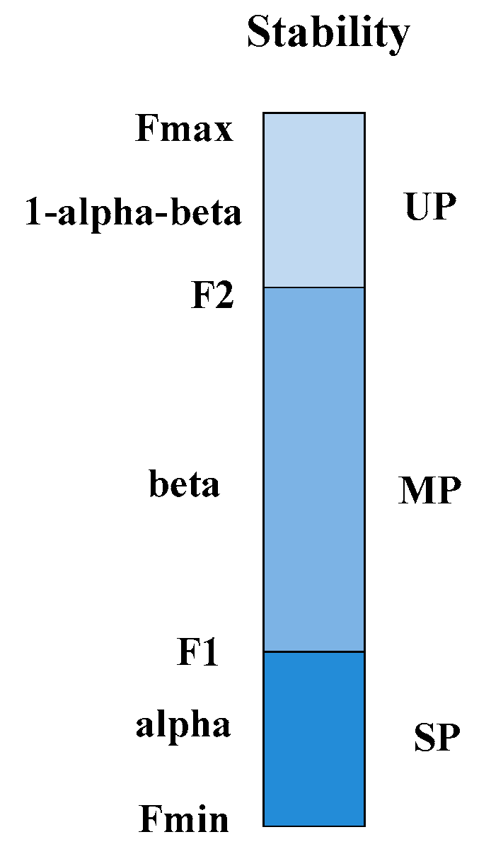
Figure 3.
A phase transition from an unstable phase to a stable phase.
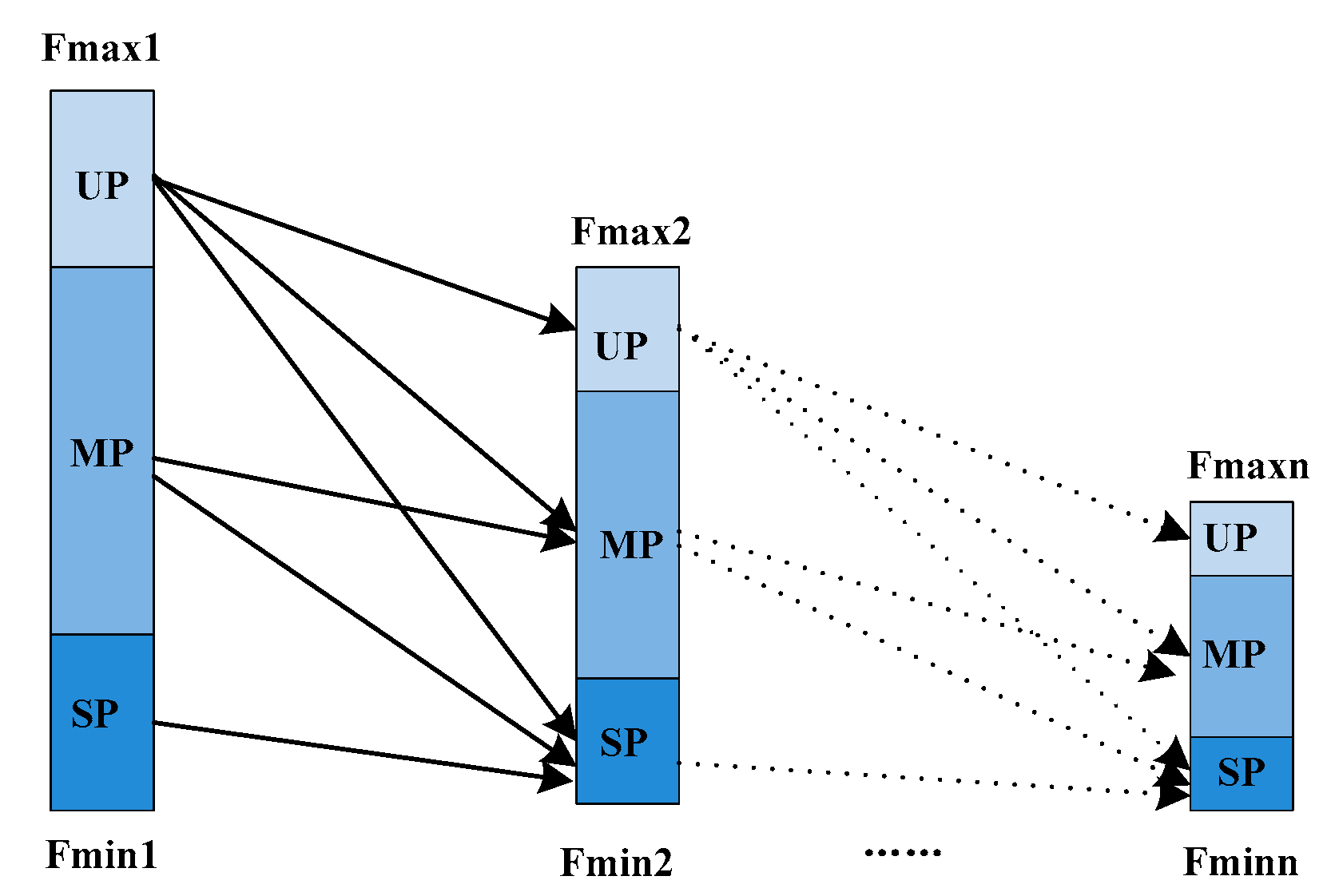
Figure 4.
Two-dimensional example showing the process of the free walking path of elements.
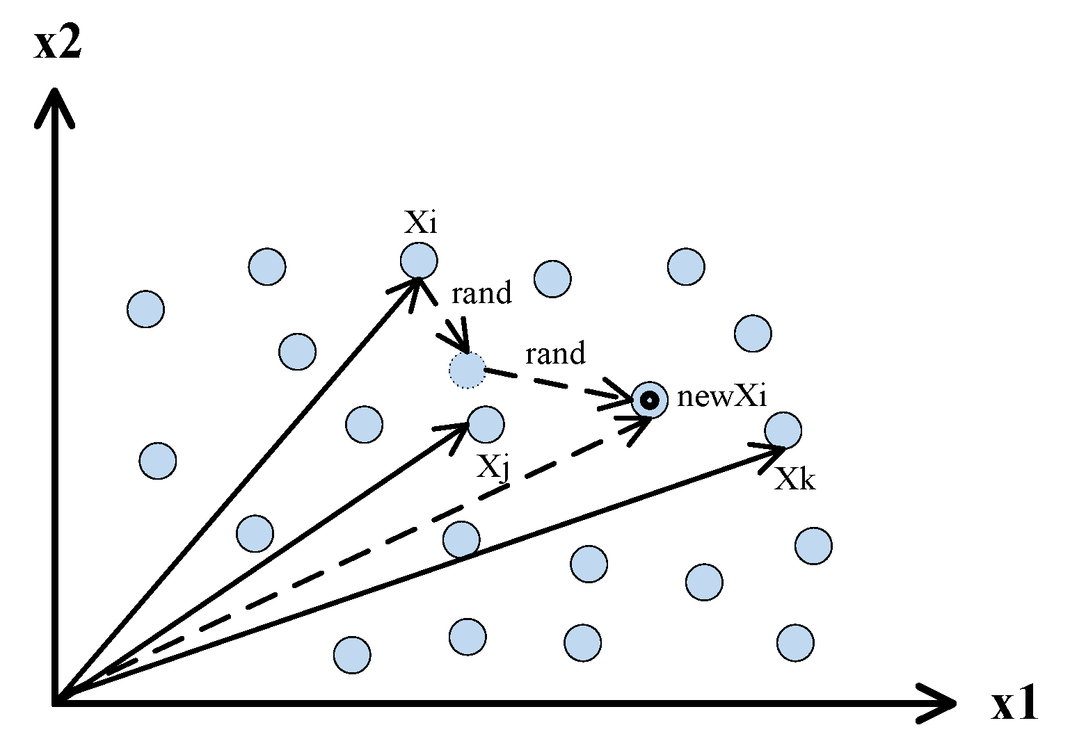
Figure 5.
The shrinkage trend of elements towards the optimal point.
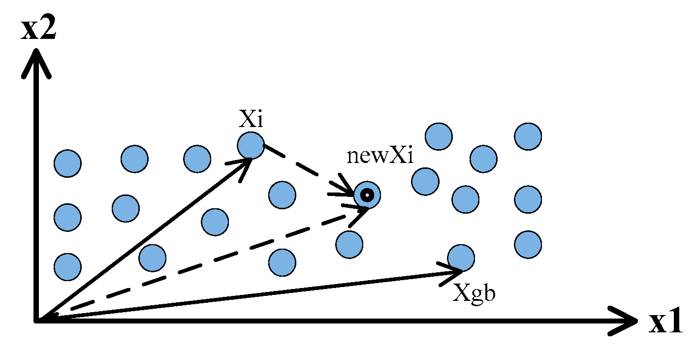
Figure 6.
The vibration of elements in an equilibrium position.

Figure 7.
The main flowchart of PTBO.

Figure 8.
Population distribution at various generations in an evolutionary process of PTBO.

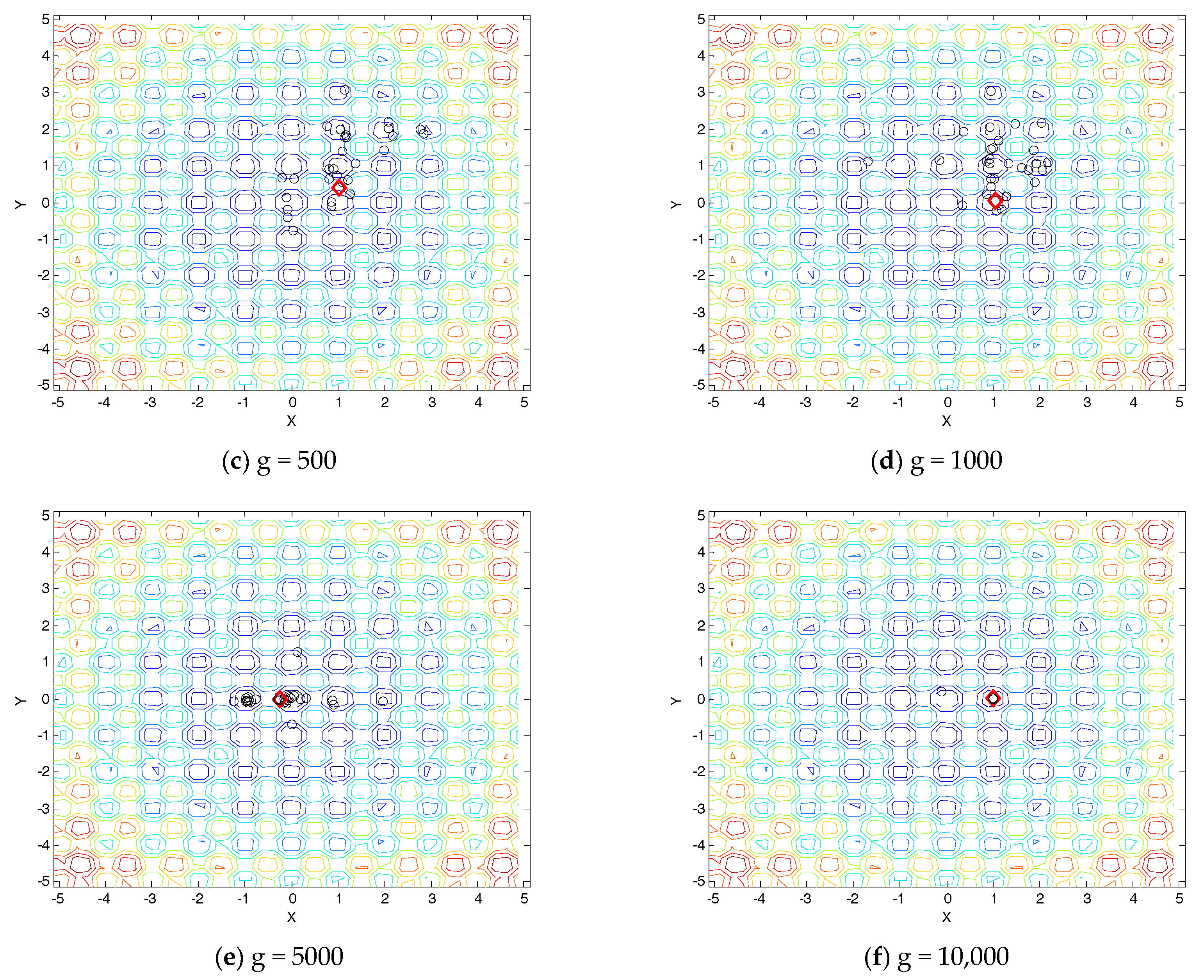
Figure 9.
Convergence performance of the compared algorithms on parts of functions.

Figure 10.
The mean central processing unit (CPU) time of the nine compared algorithms. 30D: 30 dimensions.
Figure 10.
The mean central processing unit (CPU) time of the nine compared algorithms. 30D: 30 dimensions.

Table 1.
The motional characteristics of elements in the three phases.
| Phase | Main Property | Motion Tendency | Example |
|---|---|---|---|
| UP | disorder, moving towards an arbitrary direction | stochastic motion | gaseous molecule such as water, atom, or electron in normal temperature |
| MP | between disorder and order, moving according to a certain law | shrinkage motion | liquid molecule such as water or rapid freezing alloy crystal |
| SP | order, moving in a very regular mode | vibration motion | solid molecule such as water or an atom of paramagnetic phase in a nail |
Table 2.
The relationship between the intervals and the three phases.
| Phase | Interval |
|---|---|
| UP | [Fmax, F2] |
| MP | (F2, F1) |
| SP | [F1, Fmin] |
Table 3.
The correspondence of phase transition-based optimization (PTBO) algorithm and phase transition.
Table 3.
The correspondence of phase transition-based optimization (PTBO) algorithm and phase transition.
| PTBO Algorithm | Phase Transition Process |
|---|---|
| Individual | Element |
| Population size | The number of elements |
| Fitness function | Stability degree of an element |
| Global optimal solution | The lowest stability degree of an element |
| Stochastic operator | The stochastic motion of an element in UP |
| Shrinkage operator | The shrinkage motion of an element in a MP |
| Vibration operator | The vibration and fine tuning of an element in SP |
Table 4.
Benchmark functions tested by PTBO (CEC2013).
| Type | Function ID | Functions Name |
|---|---|---|
| Uni-modal Functions | F01 | Sphere Function |
| F02 | Rotated High Conditioned Elliptic Function | |
| F03 | Rotated Bent Cigar Function | |
| F04 | Rotated Discus Function | |
| F05 | Different Powers Function | |
| Multimodal Functions | F06 | Rotated Rosenbrock’s Function |
| F07 | Rotated Schaffers F7 Function | |
| F08 | Rotated Ackley’s Function | |
| F09 | Rotated Weierstrass Function | |
| F10 | Rotated Griewank’s Function | |
| F11 | Rastrigin’s Function | |
| F12 | Rotated Rastrigin’s Function | |
| F13 | Non-Continuous Rotated Rastrigin’s Function | |
| F14 | Schwefel’s Function | |
| F15 | Rotated Schwefel’s Function | |
| F16 | Rotated Katsuura Function | |
| F17 | Lunacek Bi_Rastrigin Function | |
| F18 | Rotated Lunacek Bi_Rastrigin Function | |
| F19 | Expanded Griewank’s plus Rosenbrock’s Function | |
| F20 | Expanded Scaffer’s F6 Function | |
| Composition Functions | F21 | Composition Function 1 (n = 5, Rotated) |
| F22 | Composition Function 2 (n = 3, Unrotated) | |
| F23 | Composition Function 3 (n = 3, Rotated) | |
| F24 | Composition Function 4 (n = 3, Rotated) | |
| F25 | Composition Function 5 (n = 3, Rotated) | |
| F26 | Composition Function 6 (n = 5, Rotated) | |
| F27 | Composition Function 7 (n = 5, Rotated) | |
| F28 | Composition Function 8 (n = 5, Rotated) |
Table 5.
Different interval ratio settings of the three phases.
| Ratio Method | No. | Stable Phase | Meta-Stable Phase | Unstable Phase |
|---|---|---|---|---|
| Fixed ratio | Prop1 | 0.05 | 0.8 | 0.15 |
| Prop2 | 0.1 | 0.8 | 0.1 | |
| Prop3 | 0.15 | 0.8 | 0.05 | |
| Random ratio | Prop4 | 0.2 * rand | 0.8 | 0.2 * (1 − rand) |
Table 6.
Compared results of different interval ratios.
| Func. | Prop1 | Prop2 | Prop3 | Prop4 | Func. | Prop1 | Prop2 | Prop3 | Prop4 |
|---|---|---|---|---|---|---|---|---|---|
| F01 | 6.16 × 10⁻²⁷ | 6.13 × 10⁻²⁷ | 3.82 × 10⁻²⁸ | 4.31 × 10⁻²⁸ | F15 | 4.45 × 10³ | 4.57 × 10³ | 4.27 × 10³ | 4.23 × 10³ |
| 2.08 × 10⁻²⁶ | 3.70 × 10⁻²⁶ | 6.04 × 10⁻²⁸ | 5.96 × 10⁻²⁸ | 5.99 × 10² | 6.55 × 10² | 7.24 × 10² | 7.64 × 10² | ||
| F02 | 7.90 × 10⁵ | 8.73 × 10⁵ | 1.02 × 10⁶ | 8.63 × 10⁵ | F16 | 4.10 × 10⁻¹ | 4.71 × 10⁻¹ | 4.11 × 10⁻¹ | 3.94 × 10⁻¹ |
| 2.89 × 10⁵ | 3.25 × 10⁵ | 3.66 × 10⁵ | 6.60 × 10⁵ | 2.01 × 10⁻¹ | 2.59 × 10⁻¹ | 2.07 × 10⁻¹ | 1.96 × 10⁻¹ | ||
| F03 | 1.95 × 10⁸ | 1.12 × 10⁸ | 8.01 × 10⁷ | 3.84 × 10⁷ | F17 | 7.58 × 101 | 7.13 × 101 | 6.68 × 101 | 6.72 × 101 |
| 2.91 × 10⁸ | 1.49 × 10⁸ | 1.22 × 10⁸ | 5.22 × 10⁷ | 1.45 × 101 | 1.25 × 101 | 9.94 | 1.63 × 101 | ||
| F04 | 8.08 × 10³ | 9.03 × 10³ | 1.30 × 10⁴ | 8.26 × 10³ | F18 | 7.96 × 101 | 7.57 × 101 | 6.99 × 101 | 6.66 × 101 |
| 2.59 × 10³ | 2.35 × 10³ | 3.43 × 10³ | 3.71 × 10³ | 1.47 × 101 | 1.15 × 101 | 1.14 × 101 | 1.23 × 101 | ||
| F05 | 1.36 × 10⁻¹⁴ | 3.00 × 10⁻¹⁵ | 6.38 × 10⁻²² | 2.64 × 10⁻¹⁵ | F19 | 5.05 × 10² | 5.05 × 10² | 5.04 × 10² | 5.04 × 10² |
| 2.19 × 10⁻¹⁴ | 4.32 × 10⁻¹⁵ | 1.18 × 10⁻²¹ | 4.44 × 10⁻¹⁵ | 1.61 | 1.45 | 1.06 | 8.36 × 10⁻¹ | ||
| F06 | 2.32 × 101 | 3.09 × 101 | 2.74 × 101 | 2.53 × 101 | F20 | 1.21 × 101 | 1.19 × 101 | 1.26 × 101 | 1.15 × 101 |
| 2.57 × 101 | 2.88 × 101 | 2.58 × 101 | 2.67 × 101 | 1.68 | 2.01 | 2.07 | 2.12 | ||
| F07 | 5.30 × 101 | 5.01 × 101 | 4.13 × 101 | 3.04 × 101 | F21 | 3.01 × 10² | 3.30 × 10² | 3.22 × 10² | 2.97 × 10² |
| 2.31 × 101 | 1.90 × 101 | 1.93 × 101 | 1.73 × 101 | 7.76 × 101 | 8.86 × 101 | 7.19 × 101 | 8.01 × 101 | ||
| F08 | 2.09 × 101 | 2.09 × 101 | 2.09 × 101 | 2.09 × 101 | F22 | 1.01 × 10³ | 8.03 × 10² | 9.74 × 10² | 8.61 × 10² |
| 6.18 × 10⁻² | 6.57 × 10⁻² | 6.50 × 10⁻² | 6.50 × 10⁻² | 4.92 × 10² | 2.79 × 10² | 4.68 × 10² | 3.11 × 10² | ||
| F09 | 2.49 × 101 | 2.39 × 101 | 2.43 × 101 | 1.90 × 101 | F23 | 5.25 × 10³ | 5.16 × 10³ | 5.07 × 10³ | 4.15 × 10³ |
| 5.33 | 5.24 | 5.54 | 5.26 | 8.49 × 10² | 6.32 × 10² | 7.01 × 10² | 1.40 × 10³ | ||
| F10 | 3.50 × 10⁻¹ | 3.39 × 10⁻¹ | 3.43 × 10⁻¹ | 3.27 × 10⁻¹ | F24 | 2.42 × 10² | 2.35 × 10² | 2.33 × 10² | 2.33 × 10² |
| 2.03 × 10⁻¹ | 1.85 × 10⁻¹ | 1.73 × 10⁻¹ | 1.77 × 10⁻¹ | 8.21 | 8.66 | 8.46 | 1.04 × 101 | ||
| F11 | 4.85 × 101 | 4.05 × 101 | 3.89 × 101 | 3.92 × 101 | F25 | 2.81 × 10² | 2.79 × 10² | 2.78 × 10² | 2.74 × 10² |
| 1.60 × 101 | 1.38 × 101 | 1.12 × 101 | 1.21 × 101 | 1.34 × 101 | 1.46 × 101 | 1.32 × 101 | 1.02 × 101 | ||
| F12 | 1.40 × 10² | 1.28 × 10² | 1.21 × 10² | 6.32 × 101 | F26 | 2.53 × 10² | 2.77 × 10² | 2.48 × 10² | 2.51 × 10² |
| 2.82 × 101 | 3.41 × 101 | 3.72 × 101 | 2.51 × 101 | 6.85 × 101 | 6.93 × 101 | 6.71 × 101 | 6.57 × 101 | ||
| F13 | 1.61 × 10² | 1.53 × 10² | 1.47 × 10² | 1.18 × 10² | F27 | 7.50 × 10² | 7.41 × 10² | 7.23 × 10² | 6.38 × 10² |
| 3.13 × 101 | 2.76 × 101 | 2.67 × 101 | 3.07 × 101 | 9.33 × 101 | 1.21 × 10² | 1.34 × 10² | 1.16 × 10² | ||
| F14 | 9.52 × 10² | 8.63 × 10² | 9.35 × 10² | 9.47 × 10² | F28 | 3.93 × 10² | 3.46 × 10² | 3.51 × 10² | 2.96 × 10² |
| 3.28 × 10² | 3.31 × 10² | 3.49 × 10² | 2.81 × 10² | 4.61 × 10² | 2.74 × 10² | 3.92 × 10² | 2.83 × 101 |
Bold text is the best result obtained by different interval ratios.
Table 7.
The parameter settings of the compared algorithms.
| No. | Algorithm | Parameter Setting |
|---|---|---|
| 1 | PSO | |
| 2 | DE | |
| 3 | BA | |
| 4 | CS | |
| 5 | BSD | |
| 6 | WWO | |
| 7 | WCA | |
| 8 | SMS | Gas state: |
| Liquid state: | ||
| Solid state: | ||
| 9 | PTBO | alpha is random ratio, beta = 0.8 |
PSO: particle swarm optimization; DE: Differential Evolution; BA: Bat Algorithm; CS: Cuckoo Search; BSO: Brain Storm Optimization; WWO: Water Wave Optimization; WCA: Water Cycle Algorithm; SMS: States of Matter Search.
Table 8.
The results of solution accuracy for the uni-modal functions.
| Func. | PTBO | PSO | DE | BA | CS | BSO | WWO | WCA | SMS |
|---|---|---|---|---|---|---|---|---|---|
| F01 | 4.31 × 10⁻²⁸ | 3.56 × 10³ ǂ | 2.65 × 10³ ǂ | 1.05 × 10⁻³ ǂ | 4.46 × 10³ ǂ | 3.71 × 10⁻³ ǂ | 2.62 × 10⁻²⁸ ξ | 1.58 × 10⁻²⁸ ξ | 4.63 × 10⁴ ǂ |
| 5.96 × 10⁻²⁸ | 2.65 × 10³ | 8.98 × 10⁻¹ | 1.29 × 10⁻⁴ | 3.10 × 10² | 5.71 × 10⁻³ | 1.30 × 10⁻²⁸ | 1.45 × 10⁻²⁸ | 4.24 × 10³ | |
| F02 | 8.63 × 10⁵ | 1.12 × 10⁷ ǂ | 1.56 × 10⁷ ξ | 4.82 × 10⁴ ξ | 4.21 × 10⁷ ǂ | 1.17 × 10⁶ ǂ | 1.20 × 10⁶ ǂ | 7.53 × 10⁵ ξ | 4.91 × 10⁸ ǂ |
| 6.60 × 10⁵ | 1.56 × 10⁷ | 2.05 × 10⁵ | 1.81 × 10⁴ | 4.04 × 10⁶ | 3.35 × 10⁵ | 7.19 × 10⁵ | 7.54 × 10⁵ | 8.49 × 10⁷ | |
| F03 | 3.84 × 10⁷ | 4.98 × 10¹⁰ ǂ | 4.72 × 10¹⁰ ǂ | 8.96 × 10⁸ ǂ | 1.72 × 10¹⁰ ǂ | 1.66 × 10⁸ ǂ | 3.98 × 10⁸ ǂ | 2.94 × 10⁹ ǂ | 1.00 × 10¹⁰ ǂ |
| 5.22 × 10⁷ | 4.72 × 10¹⁰ | 3.57 × 10⁷ | 3.48 × 10⁸ | 2.11 × 10⁹ | 2.22 × 10⁸ | 6.71 × 10⁸ | 4.30 × 10⁹ | 0.00 | |
| F04 | 8.26 × 10³ | 5.64 × 10³ ξ | 8.41 × 10³ ǂ | 2.42 × 10⁴ ǂ | 6.05 × 10⁴ ǂ | 5.44 × 10³ ξ | 5.57 × 10⁴ ǂ | 6.55 × 101 ξ | 8.14 × 10⁴ ǂ |
| 3.71 × 10³ | 8.41 × 10³ | 1.27 × 10³ | 3.91 × 10² | 6.61 × 10² | 2.22 × 10³ | 1.05 × 10⁴ | 2.07 × 10² | 9.79 × 10³ | |
| F05 | 2.64 × 10⁻¹⁵ | 1.58 × 10³ ǂ | 1.25 × 10³ ǂ | 1.37 × 10⁻² ǂ | 1.09 × 10³ ǂ | 4.12 × 10⁻² ǂ | 5.53 × 10⁻² ǂ | 2.95 × 10⁻¹² ǂ | 1.38 × 10⁴ ǂ |
| 4.44 × 10⁻¹⁵ | 1.25 × 10³ | 1.84 × 101 | 2.08 × 10⁻³ | 6.70 × 101 | 1.74 × 10⁻² | 2.90 × 10⁻¹ | 7.89 × 10⁻¹² | 2.66 × 10³ | |
| ǂ/ξ/~ | 4/1/0 | 4/1/0 | 4/1/0 | 5/0/0 | 4/1/0 | 4/1/0 | 2/3/0 | 5/0/0 | |
“ǂ”, “ξ”, and “~” denote that the performance of PTBO is better than, worse than, and similar to that of the corresponding algorithm, respectively. Bold text is the best result obtained by the compared algorithms.
Table 9.
The results of solution accuracy for the multimodal functions.
| Function | PTBO | PSO | DE | BA | CS | BSO | WWO | WCA | SMS |
|---|---|---|---|---|---|---|---|---|---|
| F06 | 2.53 × 101 | 2.51 × 10² ǂ | 3.20 × 101 ǂ | 1.36 ξ | 4.99 × 10² ǂ | 4.30 × 101 ǂ | 5.51 × 101 ǂ | 3.27 × 101 ǂ | 6.18 × 10³ ǂ |
| 2.67 × 101 | 2.11 × 10² | 2.51 × 101 | 6.61 | 5.70 × 101 | 2.84 × 101 | 2.76 × 101 | 2.67 × 101 | 9.16 × 10² | |
| F07 | 3.04 × 101 | 1.19 × 10² ǂ | 2.44 × 101 ξ | 2.59 × 10⁸ ǂ | 2.51 × 10⁸ ǂ | 1.59 × 10² ǂ | 8.91 × 101 ǂ | 1.90 × 10² ǂ | 5.50 × 10³ ǂ |
| 1.73 × 101 | 4.67 × 101 | 1.43 × 101 | 4.83 × 10⁷ | 2.44 × 10⁷ | 1.11 × 10² | 3.02 × 101 | 4.00 × 101 | 3.85 × 10³ | |
| F08 | 2.09 × 101 | 2.09 × 101 ~ | 2.09 × 101 ~ | 2.10 × 101 ~ | 2.11 × 101 ~ | 2.09 × 101 ~ | 2.09 × 101 ~ | 2.09 × 101 ~ | 2.09 × 101 ~ |
| 6.50 × 10⁻² | 5.71 × 10⁻² | 4.33 × 10⁻² | 6.52 × 10⁻² | 6.15 × 10⁻² | 7.40 × 10⁻² | 5.56 × 10⁻² | 5.56 × 10⁻² | 5.31 × 10⁻² | |
| F09 | 1.90 × 101 | 2.18 × 101 ~ | 1.86 × 101 ξ | 5.77 × 101 ǂ | 5.73 × 101 ǂ | 3.42 × 101 ǂ | 2.76 × 101 ǂ | 3.40 × 101 ǂ | 4.00 × 101 ǂ |
| 5.26 | 2.73 | 4.40 | 3.29 | 1.16 | 3.72 | 4.29 | 3.01 | 1.48 | |
| F10 | 3.27 × 10⁻¹ | 7.01 × 10² ǂ | 6.65 × 10⁻¹ ~ | 1.14 ǂ | 9.05 × 10² ǂ | 9.62 × 10⁻¹ ~ | 1.41 × 10⁻¹ ξ | 3.17 × 10⁻¹ ~ | 5.60 × 10³ ǂ |
| 1.77 × 10⁻¹ | 4.13 × 10² | 1.21 | 6.95 × 10⁻¹ | 4.90 × 101 | 2.16 × 10⁻¹ | 7.49 × 10⁻² | 2.00 × 10⁻¹ | 6.76 × 10² | |
| F11 | 3.92 × 101 | 1.05 × 10² ǂ | 2.27 × 101 ξ | 9.90 × 10² ǂ | 9.90 × 10² ǂ | 6.03 × 10² ǂ | 1.22 × 10² ǂ | 1.05 × 10² ǂ | 7.65 × 10² ǂ |
| 1.21 × 101 | 5.68 × 101 | 7.87 | 2.71 × 101 | 2.24 × 101 | 1.03 × 10² | 3.80 × 101 | 4.84 × 101 | 6.72 × 101 | |
| F12 | 6.32 × 101 | 1.07 × 10² ǂ | 4.14 × 101 ξ | 9.50 × 10² ǂ | 9.52 × 10² ǂ | 5.97 × 10² ǂ | 1.36 × 10² ǂ | 3.38 × 10² ǂ | 7.63 × 10² ǂ |
| 2.51 × 101 | 3.62 × 101 | 1.21 × 101 | 1.28 × 101 | 1.34 × 101 | 1.04 × 10² | 3.51 × 101 | 9.25 × 101 | 5.78 × 101 | |
| F13 | 1.18 × 10² | 2.80 × 10² ǂ | 2.09 × 10² ǂ | 1.12 × 10³ ǂ | 1.12 × 10³ ǂ | 6.51 × 10² ǂ | 2.07 × 10² ǂ | 3.46 × 10² ǂ | 7.68 × 10² ǂ |
| 3.07 × 101 | 3.13 × 101 | 3.63 × 101 | 4.65 × 101 | 3.75 × 101 | 7.86 × 101 | 5.72 × 101 | 6.77 × 101 | 5.35 × 101 | |
| F14 | 9.47 × 10² | 2.00 × 10³ ǂ | 1.46 × 10³ ǂ | 5.72 × 10³ ǂ | 5.90 × 10³ ǂ | 4.42 × 10³ ǂ | 3.23 × 10³ ǂ | 2.37 × 10³ ǂ | 7.72 × 10³ ǂ |
| 2.81 × 10² | 6.45 × 10² | 4.71 × 10² | 4.38 × 10² | 4.38 × 10² | 7.77 × 10² | 6.47 × 10² | 7.83 × 10² | 3.88 × 10² | |
| F15 | 4.23 × 10³ | 4.02 × 10³ ξ | 7.21 × 10³ ǂ | 5.02 × 10³ ǂ | 4.99 × 10³ ǂ | 4.33 × 10³ ~ | 5.16 × 10³ ǂ | 4.72 × 10³ ǂ | 7.59 × 10³ ǂ |
| 7.64 × 10² | 6.52 × 10² | 3.53 × 10² | 2.58 × 10² | 2.57 × 10² | 6.67 × 10² | 1.72 × 10³ | 6.74 × 10² | 2.60 × 10² | |
| F16 | 3.94 × 10⁻¹ | 1.94 ǂ~ | 2.49 ǂ | 1.98 ǂ | 1.89 ǂ | 3.13 × 10⁻¹ ξ | 2.00 ǂ | 1.63 ǂ | 2.59 ǂ |
| 1.96 × 10⁻¹ | 4.89 × 10⁻¹ | 3.29 × 10⁻¹ | 9.87 × 10⁻¹ | 8.45 × 10⁻¹ | 1.16 × 10⁻¹ | 8.11 × 10⁻¹ | 4.95 × 10⁻¹ | 3.08 × 10⁻¹ | |
| F17 | 6.72 × 101 | 8.45 × 101 ǂ | 6.39 × 101 ξ | 8.29 × 10² ǂ | 8.42 × 10² ǂ | 6.10 × 10² ǂ | 1.43 × 10² ǂ | 2.39 × 10² ǂ | 1.51 × 10³ ǂ |
| 1.63 × 101 | 3.92 × 101 | 9.90 | 1.12 × 101 | 1.41 × 101 | 1.03 × 10² | 3.67 × 101 | 1.09 × 10² | 1.02 × 10² | |
| F18 | 6.66 × 101 | 1.26 × 10² ǂ | 2.92 × 10² ǂ | 8.26 × 10² ǂ | 8.33 × 10² ǂ | 5.13 × 10² ǂ | 1.42 × 10² ǂ | 4.66 × 10² ǂ | 1.53 × 10³ ǂ |
| 1.23 × 101 | 4.99 × 101 | 1.86 × 101 | 1.17 × 101 | 1.02 × 101 | 9.43 × 101 | 3.31 × 101 | 1.43 × 10² | 8.20 × 101 | |
| F19 | 5.04 × 10² | 2.16 × 10³ ǂ | 5.65 × 10² ǂ | 3.37 × 10³ ǂ | 1.55 × 10³ ǂ | 5.12 × 10² ~ | 5.16 × 10² ~ | 5.14 × 10² ~ | 5.90 × 10⁵ ǂ |
| 8.36 × 10⁻¹ | 3.38 × 10³ | 2.84 | 1.85 × 10² | 7.16 × 101 | 2.41 | 1.71 | 5.60 | 2.78 × 10⁵ | |
| F20 | 1.15 × 101 | 1.24 × 101 ǂ | 1.28 × 101 ǂ | 1.50 × 101 ǂ | 1.50 × 101 ǂ | 1.45 × 101 ǂ | 1.29 × 101 ǂ | 1.50 × 101 ǂ | 1.50 × 101 ǂ |
| 2.12 | 8.98 × 10⁻¹ | 5.20 × 10⁻¹ | 0.00 | 0.00 | 9.18 × 10⁻² | 1.00 | 0.00 | 5.71 × 10⁻² | |
| ǂ/ξ/~ | 12/1/2 | 8/5/2 | 13/1/1 | 14/0/1 | 10/1/4 | 12/1/2 | 10/3/2 | 14/0/1 | |
“ǂ”, “ξ”, and “~” denote that the performance of PTBO is better than, worse than, and similar to that of the corresponding algorithm, respectively. Bold text is the best result obtained by the compared algorithms.
Table 10.
The results of solution accuracy for the composition functions.
| Function | PTBO | PSO | DE | BA | CS | BSO | WWO | WCA | SMS |
|---|---|---|---|---|---|---|---|---|---|
| F21 | 2.97 × 10² | 4.91 × 10² ǂ | 4.20 × 10² ǂ | 3.01 × 10² ~ | 1.50 × 10³ ǂ | 3.48 × 10² ǂ | 3.25 × 10² ~ | 3.51 × 10² ~ | 3.64 × 10³ ǂ |
| 8.01 × 101 | 2.21 × 10² | 8.52 × 101 | 2.68 × 10⁻² | 8.81 × 101 | 8.87 × 101 | 8.01 × 101 | 8.51 × 101 | 2.17 × 10² | |
| F22 | 8.61 × 10² | 2.17 × 10³ ǂ | 1.33 × 10³ ǂ | 8.52 × 10³ ǂ | 8.52 × 10³ ǂ | 5.62 × 10³ ǂ | 4.09 × 10³ ǂ | 4.01 × 10³ ǂ | 8.39 × 10³ ǂ |
| 3.11 × 10² | 6.53 × 10² | 3.94 × 10² | 1.76 × 10² | 1.93 × 10² | 8.61 × 10² | 7.54 × 10² | 1.23 × 10³ | 3.46 × 10² | |
| F23 | 4.15 × 10³ | 4.16 × 10³ ~ | 6.61 × 10³ ǂ | 7.55 × 10³ ǂ | 7.74 × 10³ ǂ | 5.67 × 10³ ǂ | 5.40 × 10³ ~ | 6.64 × 10³ ǂ | 8.25 × 10³ ǂ |
| 1.40 × 10³ | 8.98 × 10² | 9.13 × 10² | 5.35 × 10² | 3.99 × 10² | 6.67 × 10² | 1.33 × 10³ | 6.71 × 10² | 2.72 × 10² | |
| F24 | 2.33 × 10² | 2.84 × 10² ǂ | 2.95 × 10² ǂ | 7.03 × 10² ǂ | 7.28 × 10² ǂ | 3.34 × 10² ǂ | 2.63 × 10² ǂ | 3.08 × 10² ǂ | 3.58 × 10² ǂ |
| 1.04 × 101 | 1.23 × 101 | 1.05 × 101 | 9.88 × 101 | 1.43 × 101 | 1.89 × 101 | 1.44 × 101 | 3.54 × 101 | 1.05 × 101 | |
| F25 | 2.74 × 10² | 3.03 × 10² ~ | 2.66 × 10² ξ | 4.48 × 10² ǂ | 4.45 × 10² ǂ | 3.56 × 10² ǂ | 3.04 × 10² ~ | 3.17 × 10² ~ | 3.73 × 10² ǂ |
| 1.02 × 101 | 9.32 | 7.55 | 2.23 × 101 | 4.24 | 1.76 × 101 | 1.47 × 101 | 1.11 × 101 | 8.47 | |
| F26 | 2.51 × 10² | 3.23 × 10² ǂ | 2.70 × 10² ǂ | 5.52 × 10² ǂ | 5.15 × 10² ǂ | 2.38 × 10² ξ | 2.00 × 10² ξ | 3.51 × 10² ~ | 2.62 × 10² ǂ |
| 6.57 × 101 | 6.95 × 101 | 7.11 × 101 | 3.00 × 101 | 3.47 × 101 | 7.46 × 101 | 3.74 × 10⁻² | 7.68 × 101 | 1.61 × 101 | |
| F27 | 6.38 × 10² | 9.62 × 10² ǂ | 7.14 × 10² ~ | 3.30 × 10³ ǂ | 2.83 × 10³ ǂ | 1.36 × 10³ ǂ | 9.90 × 10² ǂ | 1.22 × 10³ ǂ | 1.50 × 10³ ǂ |
| 1.16 × 10² | 7.94 × 101 | 7.45 × 101 | 2.89 × 10² | 8.94 × 101 | 9.72 × 101 | 1.20 × 10² | 8.93 × 101 | 4.49 × 101 | |
| F28 | 2.96 × 10² | 2.11 × 10³ ǂ | 3.00 × 10² ~ | 7.53 × 10³ ǂ | 8.82 × 10³ ǂ | 4.95 × 10³ ǂ | 5.36 × 10² ǂ | 2.03 × 10³ ǂ | 5.34 × 10³ ǂ |
| 2.83 × 101 | 5.50 × 10² | 1.09 × 10⁻¹ | 4.46 × 10² | 2.61 × 10² | 7.15 × 10² | 5.90 × 10² | 1.69 × 10³ | 4.17 × 10² | |
| ǂ/ξ/~ | 6/0/2 | 5/1/2 | 7/0/1 | 8/0/0 | 7/0/1 | 4/1/3 | 5/0/3 | 8/0/0 | |
“ǂ”, “ξ”, and “~” denote that the performance of PTBO is better than, worse than, and similar to that of the corresponding algorithm, respectively. Bold text is the best result obtained by the compared algorithms.
Table 11.
The total results of solution accuracy for the 28 functions.
| PTBO vs. | PSO | DE | BA | CS | BSO | WWO | WCA | SMS |
|---|---|---|---|---|---|---|---|---|
| F01–05 | 4/1/0 | 4/1/0 | 4/1/0 | 5/0/0 | 4/1/0 | 4/1/0 | 2/3/0 | 5/0/0 |
| F06–20 | 12/1/2 | 8/5/2 | 13/1/1 | 14/0/1 | 10/1/4 | 12/1/2 | 10/3/2 | 14/0/1 |
| F21–28 | 6/0/2 | 5/1/2 | 7/0/1 | 8/0/0 | 7/0/1 | 4/1/3 | 5/0/3 | 8/0/0 |
| ǂ/ξ/~ | 22/2/4 | 17/7/4 | 24/4/2 | 27/0/1 | 21/2/5 | 20/3/5 | 17/6/5 | 27/0/1 |
Table 12.
Wilcoxon signed-rank test of 28 functions.
| PTBO vs. | R+ | R− | p-Value |
|---|---|---|---|
| PSO | 305 | 73 | 2.69 × 10⁻⁴ |
| DE | 215 | 163 | 3.16 × 10⁻¹ |
| BA | 325 | 53 | 1.19 × 10⁻⁴ |
| CS | 368 | 10 | 3.79 × 10⁻⁶ |
| BSO | 340 | 38 | 1.57 × 10⁻⁴ |
| WWO | 359 | 19 | 2.52 × 10⁻⁵ |
| WCA | 320 | 58 | 1.20 × 10⁻³ |
| SMS | 360 | 18 | 2.96 × 10⁻⁵ |
Bold text is the best result obtained by the compared algorithms.
© 2017 by the authors. Licensee MDPI, Basel, Switzerland. This article is an open access article distributed under the terms and conditions of the Creative Commons Attribution (CC BY) license (http://creativecommons.org/licenses/by/4.0/).
Share and Cite
MDPI and ACS Style
Cao, Z.; Wang, L. An Optimization Algorithm Inspired by the Phase Transition Phenomenon for Global Optimization Problems with Continuous Variables. Algorithms 2017, 10, 119. https://doi.org/10.3390/a10040119
AMA Style
Cao Z, Wang L. An Optimization Algorithm Inspired by the Phase Transition Phenomenon for Global Optimization Problems with Continuous Variables. Algorithms. 2017; 10(4):119. https://doi.org/10.3390/a10040119
Chicago/Turabian StyleCao, Zijian, and Lei Wang. 2017. "An Optimization Algorithm Inspired by the Phase Transition Phenomenon for Global Optimization Problems with Continuous Variables" Algorithms 10, no. 4: 119. https://doi.org/10.3390/a10040119
Note that from the first issue of 2016, this journal uses article numbers instead of page numbers. See further details here.