A Comparative Study on Recently-Introduced Nature-Based Global Optimization Methods in Complex Mechanical System Design


Department of Mechanical Engineering, University of Victoria, Victoria, BC V8W 2Y2, Canada
*
Author to whom correspondence should be addressed.
Algorithms 2017, 10(4), 120; https://doi.org/10.3390/a10040120
Submission received: 9 September 2017
/
Revised: 11 October 2017
/
Accepted: 13 October 2017
/
Published: 17 October 2017
Abstract
:Advanced global optimization algorithms have been continuously introduced and improved to solve various complex design optimization problems for which the objective and constraint functions can only be evaluated through computation intensive numerical analyses or simulations with a large number of design variables. The often implicit, multimodal, and ill-shaped objective and constraint functions in high-dimensional and “black-box” forms demand the search to be carried out using low number of function evaluations with high search efficiency and good robustness. This work investigates the performance of six recently introduced, nature-inspired global optimization methods: Artificial Bee Colony (ABC), Firefly Algorithm (FFA), Cuckoo Search (CS), Bat Algorithm (BA), Flower Pollination Algorithm (FPA) and Grey Wolf Optimizer (GWO). These approaches are compared in terms of search efficiency and robustness in solving a set of representative benchmark problems in smooth-unimodal, non-smooth unimodal, smooth multimodal, and non-smooth multimodal function forms. In addition, four classic engineering optimization examples and a real-life complex mechanical system design optimization problem, floating offshore wind turbines design optimization, are used as additional test cases representing computationally-expensive black-box global optimization problems. Results from this comparative study show that the ability of these global optimization methods to obtain a good solution diminishes as the dimension of the problem, or number of design variables increases. Although none of these methods is universally capable, the study finds that GWO and ABC are more efficient on average than the other four in obtaining high quality solutions efficiently and consistently, solving 86% and 80% of the tested benchmark problems, respectively. The research contributes to future improvements of global optimization methods.
1. Introduction
Advanced optimization methods are used in engineering design to obtain the best functional performance and/or minimum production cost of a complex product or system in the increasingly competitive international market. Nature-inspired global optimization algorithms with superior search efficiency and robustness have been continuously introduced and improved to solve various complex, nonlinear optimization problems, which most traditional gradient-based optimization methods are incapable to deal with. Moreover, these nature-inspired global optimization (GO) algorithms become more useful when the objective function of the problem of interest is in implicit, black-box form and/or its derivative information of is unavailable, unreliable, or expensive to obtain. Development of the nature-inspired global optimization algorithm dated back to the introductions of the Genetic Algorithm (GA) based on Darwin’s principle of biological systems by Holland et al. [1] Since then, Ant Colony Optimization (ACO) [2], Simulated Annealing (SA) [3], and Particle Swarm Optimization (PSO) [4], as the most recognized nature-inspired global optimization algorithms have been introduced. Due to their general applicability, ease of implantation, and relatively fast convergence, GA, PSO, ABC and SA have attracted much attention in the past, and have been applied successfully for a wide range of global optimization applications. For instance, Brenna et al. [5] employed GA optimizer to carry out multi-objective optimization for train schedules with minimum energy consumption and travel time; Zhao et al. [6] proposed an improved ant colony optimization (ACO) method for the route planning of the omnidirectional mobile vehicle; and Herish et al. [4,7] applied PSO in multi-objective optimization for reliability-redundancy assignments in design.
Over the years, significant efforts have been devoted to the further developments of various global optimization methods of both deterministic and stochastic types. The deterministic approach solves an optimization problem through a predetermined sequence of searches and search points, converging to the same or very close global optimum. Direct search [8], branch and bound [9], clustering [10], and tunneling methods [11] are typical examples of this approach. Stochastic methods, including nature-inspired techniques, are based on randomly sampled search points. Therefore, their different runs may result in different optimization results due to the random nature of the search steps. These stochastic search algorithms have the capability to identify the global optimum efficiently for many optimization problems, simply using the evaluated values of the objective function without the need of its gradient information.
With the advance of computation hardware and software, computational intensive, numerical analysis and simulation tools, such as Finite Element Analysis (FEA) and Computational Fluid Dynamics (CFD), became commonly used means for evaluating the performance of a new design with many design parameters. Global optimization can be used to search through the design space of these implicit and multimodal objective functions to identify the optimal design solution in principle. However, these types of computationally expensive, black-box function optimization problems require extensive computation during each evaluation of its objective function. Conventional nature-inspired optimization algorithms, such as GA and SA, which require very large number of objective function evaluations with lengthy computation time, particularly for high-dimensional problems with many design variables, become impractical and infeasible to use.
To address this issue, a number of recently introduced nature-inspired optimization methods, such as the Artificial Bee Colony (ABC) [12], Firefly Algorithm (FFA) [13], Cuckoo Search (CS) [14,15], Bat Algorithm (BA) [16], Flower Pollination Algorithm (FPA) [17], and Grey Wolf Optimizer (GWO) [18], have been introduced with improved ability to deal with complex and high-dimensional global optimization problems [19].
This study tests and compares the performance of the aforementioned six nature-inspired GO search methods, BA, CSA, FFA, FPA, ABC and GWO, in terms of their capability of locating the true global optimum, search efficiency, and robustness in dealing with high-dimensional and computationally expensive black-box GO problems. These advanced GO methods are closely examined using a variety of test problems, ranging from benchmark test functions to real-life design optimization of complex mechanical systems. The paper begins with an overview on these relatively new algorithms, followed by a discussion on the evaluation criteria. The convergence process and results are discussed comprehensively to rank their search efficiency and robustness.
2. Notations and Symbols
Before presenting the recently introduced nature-based global optimization methods in detail, we include the definition of the symbols and notations that have been used throughout the paper in Table 1 below.
3. Nature-Inspired Global Optimization Methods
Nature-inspired Global Optimization approaches are a class of population-based methods commonly used for solving many practical global optimization problems including: GA, PSO, SA and ACO. However, these traditional GO algorithms need an enormous number of function evaluations during the search process in order to recognize the solution, and the number of search evaluations dramatically increases when the optimization problem becomes a high-dimensional problem. Hence, new effective and capable GO search methods become necessary. In recent years, a number of new search methods have been presented including the Artificial Bee Colony (ABC), the Firefly Algorithm (FFA), the Cuckoo Search (CS), the Bat Algorithm (BA), the Flower Pollination Algorithm (FPA), and the Grey Wolf Optimizer (GWO). In this section, the selected nature-inspired global optimization methods are discussed and explored in more detail. The pros and cons, as well as the applications of the six methods are also highlighted in this section. The methods have been chosen based on:
- They have been introduced in the last decade.
- They are frequently and widely used in solving many engineering globe optimization problems.
- They share many similarities in general. For instance, all these methods begin with a randomly population group and operate a fitness value to evaluate this population. They all update the population and randomly search for the optimum. They use a sharing information mechanism wherein the evolution only looks for the best solution.
- They have the potential to solve high-dimensional complex design problems especially when the number of iterations are limited.
3.1. Artificial Bee Colony Method
The Artificial Bee Colony (ABC) method, presented by Dervis Karaboga in 2005 [19], was inspired by the search behaviour of bee colonies. Honeybees use several mechanisms, such as a waggle dance, to locate food sources. The waggle dance technique is used by scout bees to share information about the source of food. Bees can quickly and precisely modify their search pattern and search space in accordance to the updated information received from other bees. In the ABC method, artificial bees are classified into three different groups: employed bees, onlooker bees, and lastly, scout bees. Each of these groups is assigned different tasks in the ABC procedure. The employed bee’s task is to visit and collect information about a source of nectar and then share it with other bees in the hive. In the ABC algorithm, the number of employed bees and the number of food sources are equal since each employed bee is linked with only one source of nectar. The onlooker bees receive the data regarding the sources of nectar from the employed bees, and then the onlooker bees select one of the sources and start to transfer the food to the hive. The scout bees fly in random directions and have the responsibility of finding new sources of nectar. In the ABC method, the possible solution corresponds to the nectar source location in which the fitness of the solution mainly depends on the related nectar amount. Furthermore, the total number of best obtained solutions is also identical to the number of employed bees or equivalent onlooker bees.
In the ABC method, a number of parameters including population size N, number of cycles (iterations), and the exploration parameter limit should be set prior to running the optimization. The number of cycles (iterations) and the parameter limits are equally important, and, to obtain the best results, should be set to their optimal values. It must be noted that in the ABC method, employed bees apply a local search to each nectar source, whereas the onlooker bees will likely update better food sources. Therefore, in the ABC algorithm, the employed bees are responsible for diversification whereas the onlooker bees are used for condensation. By implementing these three groups of bees (employed, onlooker and scout), the ABC algorithm easily escapes from minimums and improves its search efficiency. The ABC algorithm is competitive with other nature-inspired algorithms [20]; its implementation is relatively easy, and it requires only a few tuning control parameters to be set.
Due to the high efficiency of the ABC method, many researchers have used their own points of view to utilize ABC for different purposes. For instance, Gao and Liu [21], inspired by differential evolution (DE), developed a search strategy ABC/best/1 with a new chaotic initialization method with a subsequent improvement of the exploitation ability of ABC. Zhu and Kwong [22] developed a global best- (gbest-) guided ABC algorithm (GABC) to improve the search ability as well as the efficiency by using the gbest solution with the original search formula of the ABC algorithm. Li et al. [23] presented a modified ABC method (I-ABC) using the best-so-far solution, inertia weight, and coefficients to improve the search efficiency. Banharnsakun et al. [24] presented an improved search equation that causes the solution to directly converge towards the best-so-far solution rather than through a randomly selected path. Xiang and An [25] developed an efficient and robust ABC algorithm (ERABC), in which a combined solution search equation is used to accelerate the search process. Xianneng and Yang [26] introduced a new ABC method with memory (ABCM) to guide the further foraging of the artificial bees by combining other search equations to select the best solution. Garg [27] used ABC to handle reliability-redundancy allocation optimization problem. The core steps of the ABC approach can be found in the given reference [28].
3.2. Firefly Algorithm Method
Xin-She Yang proposed the Firefly Algorithm (FFA) [29] which was inspired by the flashing lights of fireflies. Almost all of the firefly species use flashing lights as an attraction communication signal between females and males. The recurring flash, the flashing rate, and the time delay between flashes are the key concepts used among fireflies to share information. Although the mechanism of flashing lights in fireflies is still largely unclear, it is obvious that this signaling system helps fireflies find food, protect themselves, and attract their prey.
FFA has become one of the most efficient global optimization algorithms and has been used in many real-life problems [29]. In FFA, the objective function is connected to the flashing light. In other words, the brightness is proportional to the best solution of an optimization problem. Brightness will assist fireflies to travel to shinier and more attractive positions in order to find the global best solution. There are three important rules in the FFA procedure:
- Fireflies are socially oriented insects, and regardless of their sex, all of them move towards more attractive and brighter fireflies.
- The amount of attraction of a firefly is proportionate to its brightness; hence, a firefly that has less brightness will travel toward one that has higher brightness. The attractiveness decreases as the space from the other firefly rises since air absorbs light. If there is no brighter firefly in the vicinity, fireflies will travel randomly in the design space.
- The brightness (light intensity) of a firefly is specified by the objective function value of the optimization problem.
In the firefly method, there are two essential keys: the variation of the light density and the formulation of the attractiveness. FFA assumes that the attraction of a firefly is determined by its shine, which is always connected with the value of the objective function: , where is the brightness of a firefly at position and is the value of the objective function. is defined as the attractiveness of a firefly i to firefly j, which is affected by the distance between them. is the attractiveness at , where is the space between two fireflies. Coefficient is the fixed light absorption value. Over the iterations, fireflies converge to the local optimal solutions. The global solution can then be obtained by comparing the local solutions. Implementation of FFA is often easier than other nature-based GO algorithms such as PSO, BA and ACO. FFA is reasonably efficient in solving many continuous complex optimization problems that are challenging to other powerful GO algorithms such as GA and PSO [30].
The Firefly algorithm has gained much attention, and, due to its simplicity, many modifications on the FFA have been achieved. Some instances of the attention that the Firefly algorithm has received are: Bhushan and Pillai [31] compared the performance and the effectiveness of FFA in dealing with nonlinear optimization problems against GA. Farahani et al. [32] employed FFA in solving continuous practical global optimization problems in dynamic environments. Younes et al. [33] implemented a hybrid FFA for solving multi-objective continuous/discrete GO problems. Talatahari et al. [34] used FFA to find the optimum design of structure design problems. Hassanzadeh et al. [35] modified FFA to deal with image processing optimization problems. Jati [36] employed FFA to solve many complicated GO problems such as TSP. Arora and Singh [37] considered the optimal choice range of FFA parameters in different numeric experiments. Bidar and Rashidy [38] improved FFA by adjusting the parameter controller in order to balance the exploitation and exploration of the algorithm. Gandomi et al. [39] introduced a hybrid algorithm by combining the Fuzzy C-Means (FCM) with FFA to improve the clustering accuracy with global optimum solutions. Farahani et al. [40] increased the efficiency of FFA by stabilizing the algorithm’s movement to direct the fireflies towards the global best if there is no better solution found.
3.3. Cuckoo Search Method
Another recent nature-inspired global optimization method is the Cuckoo Search (CS) approach developed by Yang in 2009 [41]. The CS method is based on the natural obligatory brood parasitic behaviour of cuckoo birds in integration with the Lévy flight. A cuckoo bird places its eggs in another bird’s nest to be brooded by the mother bird of another species. In some cases, other birds engage in battle with the stranger cuckoos when the other bird realizes that the eggs in her nest are not her own. In this case, the other bird either destroys the unwelcome eggs in the nest or leaves its own nest and rebuilds a new one elsewhere. Some cuckoo female species have developed a new strategy based on imitating the colours and shapes of the eggs of other birds to increase the chance of reproduction and decrease the probability of desertion by the other bird. In general, the cuckoo’s eggs hatch before the other bird’s eggs, thus the first job of the cuckoo chick is to get rid of the other bird’s eggs to increase its own chance of being fed by the resident mother bird. This knowledge of the Cuckoo bird has been used to develop the CS algorithm.
The easiest way of applying the CS algorithm is achieved through the following three steps [42]. First, every cuckoo bird places only one egg at a time in a random nest. Second, the best nests (solutions) with a good quality of eggs are selected for the next population. Third, the number of nests is constant, and the egg deposited by a cuckoo is recognized by the other bird with a probability of . Therefore, the other bird may either destroy the alien eggs or relinquish the nest and establish a new nest. The last assumption can be estimated as the fraction of the nests when new nests (completely new solutions) are substituted. In the CS method, every egg in a nest expresses a solution, and each cuckoo can only deposit one egg. This algorithm can also be used when the problem is more complex such as where each nest could hold several eggs representing a number of solutions. Further, each cuckoo can be simply considered as a random point in the design space while the nest is the memories that are used to keep the previous solutions and compare them with the next solutions.
CS is used in dealing with high-dimensional, linear and nonlinear GO problems. A recent study showed that CS is more effective and robust than PSO and GA in multi-modal objective functions [41,42]. This is partly due to the fact that there are a limited number of parameters to be adjusted in the CS method compared to other GO algorithms such as PSO and GA. A comprehensive description of the structure of the CS method is available in [42].
Since the development of the CS method in 2010, several studies have been introduced to improve its performance. Walton et al. [43] modified the CS algorithm to be more effective in handling nonlinear GO problems such as mesh generation. Yildiz [44] employed the CS algorithm to find the optimal parameters for a machine in the milling process. Vazquez [45] used the CS algorithm with artificial neural network model can to deal with different linear and non-linear problems. Kaveh and Bakhshpoori [46] applied the CS algorithm in designing steel frames. Chifu et al. [47] used a modification of the CS algorithm to optimize the semantic web service. Tein and Ramli [48] proposed a discrete CS algorithm to solve nurse scheduling problems. Choudhary and Purohit [49] applied the CS algorithm to solve software data generation problems. Bulatovic’ et al. [50] applied the CS algorithm in handling a six-bar optimization problem. Speed [51] modified the CS algorithm to be used efficiently in dealing with large-scale problems.
3.4. Bat Algorithm Method
The Bat Algorithm (BA) is a mature nature-based algorithm proposed by Yang based on prey tracking behaviour [52]. Using the concept of echolocation, bats create sounds while flying about hunting for food. These sounds are reflected to the bat providing useful information about the targets. This mechanism enables bats to identify the type of the objects, the distance from the target, and the kind and speed of the prey. Bats have the capability to establish three-dimensional pictures around the hunting area using their advanced echolocation strategy [53,54].
While hunting, bats move randomly with velocity at location sending pulses with a range of frequency (wavelength of and loudness ) while searching for prey. Bats can control the frequency pulses and regulate the rate of pulse emissions where expresses that there are no emissions, and expresses that the emissions of bats are at their maximum power. In BA, the loudness can be controlled from maximum (positive) to the lowest value. Note that expresses that a bat has reached its target and has stopped releasing any sounds. In BA, is the best so far global solution and is obtained from among all achieved solutions. The value of depends on the size of the design space. The higher the frequency, the shorter the wavelength and the shorter the traveled distance. Bats use a limited range of frequencies from 200 to 500 kHz. The steps of BA are described in [53,54,55].
BA is known as a very robust and efficient method in dealing with many engineering optimization problems [56]. Although many publications on this algorithm exist, BA still attracts a great deal of interest from scientists and is used in a wide range of applications. Many researchers studied BA to ensure that it is able to avoid becoming trapped into local minima. For instance, Xie et al. [57] introduced a combination of Lévy flight with the BA (DLBA). Lin et al. [58] presented another hybrid of Lévy flight and bat approach (CLBA) for parameter approximation in a nonlinear dynamic model. Yılmaz and Kucuksille [59], motivated by the PSO algorithm and the ABC algorithm, proposed an improved bat algorithm (IBA) to advance the exploration mechanism of the algorithm. Wang and Guo [60] integrated the harmony search (HS) method into BA, and developed a hybrid metaheuristic (HSBA) method to increase the convergence speed of BA. Zhu et al. [61] improved the exploration capability of BA by modifying its equations. Afrabandpey et al. [54] introduced the chaotic sequences into BA in order to escape local convergence. Gandomi and Yang [62] replaced the four parameters in BA by different chaotic systems to increase the global search capability of BA. Kielkowicz and Grela [63] introduced some modification to the Bat Algorithm to solve nonlinear optimization.
3.5. Flower Pollination Algorithm Method
The Flower Pollination method (FPA) is stimulated by the nature of flower pollination [64]. The main objective of flower pollination is reproduction. Pollination occurs in two main ways: abiotic and biotic. The majority of flowers use biotic pollination, where a pollinator such as a bee, a fly or a bird transfers pollen. In some cases, flowers and insects have special cooperation, where flowers catch the attention of and rely solely on a certain species of insect to ensure an effective pollination process. Abiotic pollination is the result of wind and moving water and does not need any pollinators [64].
Self-pollination and cross-pollination are only two methods of flower pollination [65]. Self-pollination can happen when pollen is transferred from the same flower or to a different flower on the same plant when no pollinator is available. Therefore, this is considered to be a local solution. Cross-pollination happens when pollination transfers from the flowers of another plant. Biotic, cross-pollination can happen with long distance pollination and can be achieved by pollinators as a global solution. Those pollinators can behave as Lévy flight obeying Levy distribution steps. Hence, this behaviour was used to design FPA. In FPA, is considered to be the flower pollen population, where indicates the current iteration, and the parameter is the density of the pollination. In FFA both local search and global search can be adjusted by changing the probability between in order to reach the optimum solution. The mechanisms described above are formulated into mathematical expression in order to solve any optimization problem of interest. FPA has many advantages in comparison to other nature-inspired algorithms—in particular its simplicity and flexibility. Moreover, FPA requires only a few tuning parameters making its implementation relatively easy. PA has been efficiency adapted to deal with a number of real-world design GO problems in engineering and science. Alam et al. [66] used FPA for solving problems in the area of solar PV parameter estimation. Dubey et al. [63] modified FPA to deal with the fuzzy selection of dynamic GO problems. Yang et al. [17] extended FPA to solve multi-objective GO problems, developing a multi-objective flower pollination algorithm (MOFPA). Henawy et al. [67] introduced a hybrid of FPA combined with harmony search (FPCHS) to increase the accuracy of FPA. Wang and Zhou [68] presented a new search strategy called a Dimension by Dimension Improvement of FPA (DDIFPA) to enhance the convergence speed and solution quality of the original FPA. Kanagasabai et al. [69] integrated FPA with PSO (FPAPSO) to deal with reactive power dispatch problems. Meng et al. [70] presented a modified flower pollination algorithm (MFPA) while attempting to optimize five mechanical engineering design problems. Binh et al. [71] proposed the Chaotic Flower Pollination Algorithm (CFPA) to overcome the large computation time and solution instability of FPA. Łukasik et al. [72] studied FPA in solving continuous global optimization problems in intelligent systems. Sakib et al. [73] also presented a comparative study of FPA and BA in solving continuous global optimization problems. The main steps and the mathematical equations of FPA are explained in detail in [17].
3.6. Grey Wolf Optimizer Method
The Grey Wolf Optimizer (GWO) approach is a recently proposed algorithm by Seyedali [74] and is based on the behaviour of grey wolves in the wild [18,74]. GWO simulates the leadership policy and hunting strategy of a grey wolf’s family in its natural habitat. GWO is similar to other nature-inspired population-based approaches such as GA, PSO and ACO. In a family of grey wolves, there are four different groups: alpha, beta, delta and omega. The alpha, which is always male, is in charge of making decisions in hunting, selecting rest and sleeping places, etc., and its decisions must be obeyed by the rest of the family. Due to its dominating role, alpha is placed at the top of the family pyramid. Beta is at the second level in the family, and its duty is to support the alpha’s decisions or other family initiatives. Beta can be female or male, and, because of its experience working alongside the alpha, can replace the alpha if it becomes necessary. Beta acts as a counsellor to the alpha and ensures that the alpha’s orders are applied in the community, while at the same time, it guides the lower-level wolves. Further down the pyramid is the Delta which must follow the orders of the alpha and beta wolves but has domination over the omega. The duty of the delta is to defend and provide safety to all family members [75]. Omega is the lowest ranked among the grey wolf family and plays the role of scapegoat. Omegas are the last group of the grey wolf family to eat from the prey, and its duty is to take care of the new born pups. These three groups are used to simulate the leadership hierarchy in the grey wolf family. The first three groups lead omega wolves to search the space. During this search, all members update their positions according to the locations of the alpha, beta and delta.
In GWO, there are three steps of hunting which must be realized: finding prey, surrounding prey, and finally attacking and killing prey. Through the optimization procedure, the three most effective candidate solutions are alpha, beta and delta, as they are likely to be at the location of the optimal solution. Meanwhile the omega wolves must relocate with respect to the location of the other groups. As laid out in the GWO algorithm, alpha is the fittest candidate, but beta and delta gain better information about the potential position of prey than omegas. Accordingly, the best three solutions are saved in the database, while the rest of the search agents (omegas) are obliged to update their position according to the position of the best solution so far. In GWO, is the wolf population, indicates the number of iteration, and are random parameters , , represents the location vector of the prey, is the location of the agent, and is a random value to update position.
The GWO algorithm is recognized as being a capable and efficient optimization tool that can provide a very accurate result without becoming trapped in local optima [76]. Because of its inherent advantages, GWO is used in several optimal design applications. Kamboj et al. [77] successfully applied GWO in solving economic dispatch problems. Emary et al. [78] dealt with feature subset selection problems using GWO. Gholizadeh [79] utilized GWO to find the best design for nonlinear optimization problem of double layer grids. Yusof and Mustaffa [80] developed GWO to forecast daily crude oil prices. Komaki and Kayvanfar [81] employed GWO to solve scheduling optimization problems. El-Fergany and Hasanien [82] integrated GWO and DE to handle single and complex power flow problems. Zawbaa et al. [83] developed and applied a new version of GWO called the binary grey wolf optimization (BGWO) to find the optimal zone of the complex design space. Kohli and Arora [84] introduced the chaos theory into the GWO algorithm (CGWO) with the aim of accelerating its global convergence speed. Mittal et al. [85] proposed a modified grey wolf optimizer (MGWO) to improve the exploration and exploitation capability of the GWO that led to optimal efficiency of the method. GWO implementation steps are referenced in [18,81].
4. Benchmark Function and Experiment Materials
The most significant collections of global optimization benchmark problems can be found in [18,86,87]. Each benchmark problem has its individual characteristic, such as whether it is a multimodal, a unimodal or a random shape function as illustrated in Figure 1. The collection of the properties of these functions defines the complexity of benchmark problems. A problem is considered to be unimodal when it has only a local minimum which is also the global optimal, and it is classed as a multimodal when it has many local minima. The optimization problem is more difficult when the problem is non-convex or multimodal. In the search procedure, the neighborhood around local minima should be avoided as much as possible so that the optimizer does not get stuck in local minima regions. If the problem has many local minima that are randomly distributed in the design space, the problem is extremely challenging. Another significant factor that defines the complexity of the optimization problem is the number of dimensions found in the design space. Table 2 lists benchmark problems employed for the efficiency evaluation of the above optimization algorithms. The table includes name, range, dimension, characteristics and formulas of the benchmark functions. The benchmark problems used in this work have been widely used in the literature to provide a deep understanding of the performance of these six nature-based optimization algorithms.
5. Experiments
Benchmark functions are used to assess the robustness and effectiveness of optimization algorithms. In this paper, fifteen benchmark functions, as computationally-expensive black-box functions with different properties and characteristics, are used to evaluate the efficiency of the aforementioned optimization approaches. In this regard, three experiments are performed. The first experiment compares the performance among the six discussed procedures (ABC, FFA, CS, BA, PFA, and GWO) while the iteration number is restricted. The second experiment tests the consequences of increasing the dimensions of the problem on the efficiency of the algorithm. The final experiment observes the sensitivity of the CPU time needed to obtain the global solution to the number of design variables (dimensional) change.
Experiment 1.
The purpose of this experiment is to compare the optimization algorithms in terms of the efficiency when only a limited number of function evaluations (NFE) are available. In order to have unbiased comparisons, all approaches are restricted to the same iteration number (1000) as well as the same population size (40).
Experiment 2.
The impact of increasing the number of variables on the resultant accuracy of the above algorithms is examined for fifteen high-dimensional benchmark functions considered as computationally expensive black-box problems. The selected benchmark problems with their properties are shown in Section 3.2.
Experiment 3.
The computation time needed for solving computationally-expensive black-box problems is the most important matter in assessing the efficiency of an algorithm. In this experiment, the above algorithms are also compared in terms of the computation (CPU) time required to reach the global solution on the same set of benchmark problems with different numbers of design variables (dimensions).
5.1. Setting Parameters in the Experiments
The setting of parameters is indeed an essential part of applying these algorithms, affecting the outcome of the search. It is imperative to set the parameters associated with each approach to its most appropriate values to obtain the best performance of the algorithms. Generally, these parameters are found prior to implementing the algorithm and remain unchanged during execution. Several studies indicate that the best mechanism for selecting parameters is based on intensive experiments to reach the optimal parameters of any algorithm [88]. Yang X-S [89] has conducted a number of runs to select the optimal setting parameters of BA. In the ABC algorithm, Akay and Karaboga [90] have suggested efficient parameters to obtain the best results of ABC. Yuan et al. [91] have recommended better parameter values in order to enhance the efficiency of FFA and converge the global optimum. Wang et al. [92] have provided the optimal setting parameters of CS to solve the problem of Chaotic Systems in order to gain the best performance of the CA method. Yang [93] has carried out parametric studies to obtain the best values for setting parameters of FPA. Rodríguez and Castillo [94] have proposed the optimal setting parameters of the GWO to achieve the best performance of the GWO approach. The setting parameters used in Table 3 of this paper are selected based on the studies mentioned in this section.
5.2. Experiments Results
In this section, the optimization methods are compared against each other in terms of efficiency, capability and computational complexity using the fifteen high-dimensional benchmark functions. Although the overall performance of an optimization algorithm changes depending on setting parameters and other experimental criteria, benchmark problems can be used to indicate the efficiency of the algorithm under different levels of complexity. The statistical significance results from experiments on the selected benchmark functions are presented in Table 4. From Figure 2 to Figure 10 present only the results for the constrained benchmark functions with different surface with D = 25, 40 and 50. The outcome of this study may not reflect the overall efficiency of the tested algorithms under all conditions.
All experiments are conducted using a PC with a processor running at 2.60 GHz and 16 GB RAM in MATLAB R2015b running under Windows 8.1. It should be mentioned that the results are based on 25 independent runs for functions f1 to f15, with a population size set at 40 and the maximum number of iterations fixed at 1000. In these experiments, the basic versions of the selected algorithms are considered without further modification. All methods codes are obtained from different sources, and adjusted to be harmonic with our work objectives [18,28,93].
6. Discussion
In this section, the statistical results obtained in this study are compared and discussed in detail broken down by the target criteria in Section 5.
6.1. The Accuracy with Limited Number of Iterations
In this experiment, the impact of a limit of the number of iterations as well as the number of function evaluations (NFE) on the accuracy of the results of the algorithms are analyzed. Figure 2, Figure 3 and Figure 4 show the optimal solution found by BA, CSA, FFA, FPA, ABC and GWO methods versus the iteration number for three computationally-expensive problems. The selected functions are Sphere (f1), Griewank (f7) and Cigar (f14), which represent unimodal, multimodal and tough shape functions. The primary goal is to measure the performance of these algorithms based on different surface topologies/structures. The accuracy is measured by comparing the obtained optimum with the known actual optimum of the function. The evaluated efficiency is based on the convergence rate of these algorithms under the given conditions. The algorithm that yields accurate global solutions in a shorter computation time is the efficient and robust method.
As illustrated in Figure 2, Figure 3 and Figure 4 (i.e., Sphere, Griewank and Cigar), GWO, followed by ABC, have shown the best performance among the examined algorithms regardless of the function form used. GWO starts to quickly converge to the global solution within approximately 100 iterations, while the other algorithms require a higher number of iterations to find the region where the global solution may exist. The ABC algorithm also demonstrates its superior efficiency in terms of the accuracy of the solution. This is, perhaps, because of the GWO’s and ABC’s search mechanism that prevents them from easily getting trapped in local optima. GWO reaches the global solution (6.14 × 10−56, 0 and 3.51 × 10−101 respectively) with a very smooth convergence rate, and ABC is the second best (5.60 × 10⁻⁵, 1.96 × 10⁻¹⁰ and 2.14 × 10⁻¹²) as shown in Table 4. On the other hand, BA and FPA show the lowest convergence rates with comparably low efficiencies. It appears that BA and FPA require a higher number of iterations to converge to the global solution. This may be because of the poor exploration ability of BA. In addition, the multidimensional objective problem can affect the convergence rate and the accuracy of the solutions obtained by PFA [17]. This result implies that BA, FPA and also CSA are potentially more efficient in solving low-dimensional computationally-expensive optimization problems.
The performance of any algorithm typically depends upon how well the algorithm can balance the exploitation and exploration mechanisms. With intensive exploitation and poor exploration ability, algorithms such as BA easily get trapped into the local minima, whereas GWO and ABC show a much better performance, especially on the functions with a large number of local minima. CSA and FFA do not perform as well as GWO and ABC in terms of convergence rate and search efficiency and need more iterations to reach the global optima. The poor effectiveness of FFA may be due to the fact that its parameters are fixed during the search process [44] making it more likely to get trapped in local solutions. ABC shows the best performance in all cases except in f2, f4 and f12 functions, where GWO is the best performing approach, except in f13, f15. Using the Zakharov problem as an example, GWO manages to reach a minimum value of 3.85 × 10−38, which can be considered to be zero, whereas ABC finds a local solution of 105.886. From the results shown, it is clear that GWO shows a superior performance and robustness in handling high dimensional optimization problems when the number of function evaluations is limited.
6.2. The Computational Complexity Analysis
Figure 5 compares these six optimization methods in terms of the required computation time to find the optimum value, using various benchmark functions with different numbers of design variables. The computation time needed to converge is the most significant factor for any method when examining its efficiency. The number of function evaluations (NFE) required by each algorithm on a set of benchmark test functions places the computation time of the six optimization methods under investigation. Figure 5 and Table 3 indicate that GWO and FFA need the lowest and highest average CPU time respectively. As an example, in Figure 5 for functions f7 and f13, the FFA method demands a 6 and 7 times higher computation time in comparison to the ABC and GWO approaches. The computational complexity results shown in Figure 5 depict that ABC is more efficient than GWO as its CPU time is almost 50% of GWO for function f3. ABC shows good efficiency most of the time; however, it can sometimes get stuck into local minima. BA, CSA, FFA and FPA show better performances on low-dimensional problems compared to when it is dealing with high-dimensional GO problems. The GWO algorithm requires the least computation time, suggesting that GWO is the most promising global optimization method for computationally-expensive black-box problems.
The influence of increasing the number of variables on the CPU time is presented in Figure 6 and Figure 7. As shown, when the number of variables increases, FFA and CSA yield a higher computational complexity compared to the other methods. Furthermore, BA is less sensitive to increasing the number of variables than the other methods while its accuracy is less. Comparing GWO and ABC, to ascertain the best algorithms, shows that GWO needs a relatively lower CPU time, making this algorithm an efficient method for solving many practical GO problems with expensive objective function and constraints.
6.3. The Impact of Increasing the Number of Variables on the Performance
The aim of this section is to study the impact of high dimensionality on the reliability and accuracy of the solutions achieved by the tested optimization algorithms in solving computationally-expensive complex optimization problems. Figure 8, Figure 9 and Figure 10 compare the performance of these six methods for the Sphere, Griewank and Dixon and Price functions. The horizontal axis shows the number of variables, and the vertical axis shows the objective function’s error value at a fixed number of function evaluations. Similarly, the value obtained in each iteration serves as a performance indicator. As illustrated, increasing the number of variables leads to the degradation in the performance of BA and FPA. This is owing to the fact that the exploitation capability of BA is comparatively low-especially for high- dimensional problems. The results also reveal that FPA is only efficient in handling low-dimensional expensive black-box functions design problems (less than 10 design variables). On the other hand, GWO and ABC are not as sensitive as the other methods in handling high-dimensional problems regardless of the complexity and the surface topology of the tested problem. Figure 8, Figure 9 and Figure 10 show that the performance of the GWO and ABC algorithms, which is related to capability and efficiency, is superior for high-dimensional problems. Figure 10 illustrates that the FFA and CS methods continue to provide comparable and acceptable solutions regardless of the complexity of the optimization problem. Furthermore, the results indicate that the performance of these algorithms is roughly similar for low-dimensional unimodal problems (D < 10). In summary, the dimensionality strongly affects the performance of most algorithms; however, it seems that ABC is more stable as the dimension of the problems increases which is probably a result of the greater exploration ability of the ABC algorithm.
6.4. The Overall Performance of the Methods
The overall results obtained in Table 4 can be evaluated based on the properties of the selected benchmark functions. GWO outperforms other algorithms by successfully obtaining the global optimum in 13 out of 15 cases, followed by ABC which outperforms others in 12 out of 15 cases. The third and the fourth best algorithms are FFA and CSA with 9 and 6 respectively out of 15 successful convergence functions, while both BA and FPA solve only 4 of the 15 problems. In terms of accuracy, results suggest that GWO is the best performing approach in all three cases. However, in terms of the required computation time, ABC is superior to the others with an average computation time of 0.2369 seconds, followed by GWO with an average of 0.3136 s. Despite its simplicity, FFA is limited by its tendency to get trapped at local minima, mainly because of its relatively weak global search capability with complex and multimodal problems. That being said, FFA provides excellent solutions in most optimization problems in this work. In addition, BA shows a poor performance in this study, mainly due to some insufficiencies at exploration and the required high number of function evaluations. Yang [93] BA has been effectively used to handle many challenging GO issues such as multimodal objective problems. Moreover, FPA, known to be a highly efficient method with low-dimensional problems, becomes problematic with high-dimensional problems. Finally, the CS algorithm shows a good performance on number of benchmark tested function. However, the algorithm becomes inefficient when objective function evaluation represents a significant computational cost such as CFD problems. In conclusion, although this study shows GWO and ABC have the highest convergence rates with acceptable computational costs, there is, as yet, no universal algorithm capable of obtaining the global solution for all kind of problems. More research is needed to be carried out to solve computationally-expensive black-box problems. Table 4 presents the overall performance of the tested algorithms under different levels of complexity and dimensionality in order to examine their efficiency and robustness.
7. Further Tests Using Nonlinear Constrained Engineering Applications
After testing the methods with fifteen unconstrained high-dimensional benchmark functions, four non-smooth constrained engineering design GO problems were selected to examine the effectiveness of these methods in practice and identify their advantages and drawbacks. These comprised four structural design applications, involving the Welded Beam Design (WBD), the Tension/Compression Spring Design (TSD), the Pressure Vessel Design (PVD) and the Speed Reducer Design (SRD) [1]. Several authors in [1,15,95,96,97,98] have solved these problems using different methods such as the hybrid PSO-GA algorithm, the artificial bee colony, etc. All four of these selected constrained engineering problems have been considered to be computationally-expensive black-box problems. The problems chosen have design variables ranging from 3 to 7 with 4, 7, 4 and 11 constraints, respectively. An average of 25 independent runs were performed per problem, with a total of 20,000 NEF in each run. All algorithms were tested with the same stopping conditions to ensure that their convergence rate, efficiency and computation time would be examined using the same parameters. Figure 11 shows the welded beam design problem where ABC started the search with lower function values; however, it required additional time to converge, along with the algorithm, to the global minimum.
In relation to the tension/compression design problem, Figure 12 shows that GWO outperformed other optimization algorithms, converging to global solution after only a few NFE. In addition, when compared to the other algorithms, GWO converged to global optimal with the least computation time and yielded better minimum values. In the pressure vessel problem, FPA had the best performance, with the lowest standard deviation value. FPA yielded the best global optimum function value, taking more computation time to converge in comparison to BA which had the lowest CPU time.
Figure 13 compares the required CPU time in dealing with the four selected constrained optimization problems. The obtained statistical results were analysed and compared to find out the performance of the algorithms when dealing with constrained problems. The results in Table 5 have shown that:
- ABC consistently requires lower NFE than the other algorithms.
- GWO performs well in TSD, WBD and PVD cases, but it seems that the GWO needs more iterations to reach the exact global solution in the SRD case.
- Results demonstrate that the other tested algorithms are sensitive when the number of variables increases, but they can provide competitive search efficiency in some problems.
We conclude that there is no specific superior optimization algorithm that can perform well for all engineering design problems. Clearly, an algorithm may work well for a specific engineering design problem and fail on another problem. The statistical results obtained are shown in Table 5.
8. Real-life Application (Cost for Floating Offshore Wind Turbine Support Structures (FOWTs))
Wind energy technology is growing rapidly at commercial scales and is one the mature means of renewable energy generations [99]. At the coastlines, higher wind speed resources are available and they provide consistent wind power. Therefore, offshore wind turbine technologies require floating platforms to harvest the wind energy in deep waters instead of using fixed structures which are suitable for shallow waters [100]. This section provides a real life application for a group of optimization algorithms to evaluate FOWTs support structure cost based on the method reported in [100]. A spar buoy platform is one of the structures that is currently used in offshore wind projects and has been selected in this study for cost analysis as shown in Figure 14.
The approach used in this paper is to define a design parameterization for the support structure as well as a linearized frequency domain dynamic model which evaluates the stability of the floating system using the NREL 5 MW offshore wind turbine [100,101]. The support structure parametrization pattern used in this work provided the spar buoy platforms with a limited number of design variables. Hence, four design parameters are defined to shape the platform and mooring system: a central cylinder with a draft, HI, cylinder radius, RI, top tapper ratio, TI, and a catenary mooring system, XM for spar buoy platforms. Note that a free board (FB) of 5 m is used for all the spar buoy platform designs as a constant parameter. The geometric design variables are summarized in Table 6 and Figure 15. In this work, the mooring system design variable, XM defines the angled taut line and slack line configurations for the spar buoy platform. Three lines are used for this platform and they are located at the middle the cylinder height as presented in Figure 15. The anchor position is defined by the mooring variation of XM from positioning under the platform to the horizontal spread of the lines. The mass properties for each spar buoy platform are determined using the platform and mooring design parameters. The mass of support structure is calculated using a wall thickness of 50 mm using a steel density of 8050 kg/m3.
In this study, the cost of the FOWT design is defined based on three main components which include the mooring line, the 5 MW wind turbine, and the floating platform. To determine the stability of the floating system in a given environmental condition, the linearized characteristics of the hydrodynamics and aerodynamics of the FOWT must be collected in a frequency domain dynamic model. For floating platform hydrodynamics, the added mass, damping, and hydrostatic loads are calculated using WAMIT. The wind turbine dynamic characteristics are kept constant in this study. However, FAST is used to calculate the linearized dynamic properties for the NREL 5 MW offshore wind turbine. These properties include linearized stiffness, mass, and damping matrices of the offshore wind turbine in a given wind speed. Like the floating platform hydrodynamics, linearized mooring line properties can be added to the frequency domain dynamic model using a quasi-static mooring subroutine of FAST. All the calculated coefficients and loads are collected into a 6 × 6 system stiffness, mass, damping to generate the linearized frequency domain equation of motion for a FOWT Equation (1). The stability of the system is evaluated by calculating the complex response amplitude operator (RAO) for all modes of motion. More details about the dynamic model and platform parameterization can be found in [101].
The performance of the FOWT in this study is defined as the standard deviation of nacelle acceleration and is shown below:
where is the wave spectral density, and is the fore-aft nacelle acceleration response amplitude operator. The complex forms of the nacelle displacement and nacelle acceleration are given by Equations (4) and (5):
where is the wind turbine hub height. In Equations (4) and (5) the includes the aero dynamic effects of the wind turbine implicitly from the linearized dynamic properties of the wind turbine. The objective function to optimize in this study is the support structure cost including mooring system, anchor and floating platform costs:
The floating platform cost is defined as a function of the design parameters as shown in Table 7. In this study, the platform cost contains the materials, manufacturing, and installation costs using a constant cost factor of $2.5/kg [100,101]. The mooring system cost is calculated using the length of the mooring lines and the maximum steady state mooring line tension with a factor of $0.42/m kN. The anchor cost is the third component of the cost model that includes the installation and technology costs. The drag embedment anchor technology is selected in this study for catenary mooring system. Therefore, the installation cost for each anchor is defined as 100 $/anchor/kN and the technology cost is based on 5000 $/anchor.
In this study, a number of constraints are also applied to the objective function. To avoid expensive design configurations, a constraint limits the cost of the platform to less than $9 M. The performance metric is also limited to less than 1. In addition, to avoid the floating platform turning over, the steady state pitch angle of the platform should be less than 10°. The expression of this constraint is given in the following equation:
where is the steady thrust load, is the mooring line pitching moment, is the pitching moment from the ballast mass stabilizers, is the platform displacement, is the center of buoyancy of the platform, is the total mass of the FOWT, is the center of gravity location, is the water plane moment of inertia in platform pitch motion, is the mooring lines stiffness in pitch motion, is the mooring line stiffness in pitch-surge motions, and is the fairlead depth in pitch motion. For details of each constraint, the reader is referred to the study presented in [101].
The optimization methods have been tested on this real-life engineering optimization problem. The exploration space for the various platform concepts helps identify the effective cost of structure for FOWTs. In order to obtain solid results, 25 independent runs have been performed. The test results are given in Table 7 and the convergence history of each method is illustrated in Figure 16. The ABC method still provides outstanding performance and could find the global optimum within 951 function evaluations of the original functions in this case study. According to the results from previously published performance tests [101], the obtained optima are sufficiently accurate and the recorded NFEs are much lower. Figure 17 compares the optimization methods in terms of the required CPU time.
9. Conclusions
New and advanced GO algorithms have been continuously introduced to solve complex design optimization problems. These problems are characterized by using computation intensive numerical analyses and simulations as objective and constraint functions with a large number of design variables, forming the so-called computation intensive, black-box GO problems. The relatively new, nature-inspired global optimization methods, Artificial Bee Colony (ABC), Firefly Algorithm (FFA), Cuckoo Search (CS), Bat Algorithm (BA), Flower Pollination Algorithm (FPA) and Grey Wolf Optimizer (GWO), have been introduced to improve search efficiency by reducing the needed number of objective function evaluations and increasing the robustness and accuracy of the results. This study is aimed at gaining a better understanding of the relative overall performance of these six well-known new GO search methods. The systematically conducted comparative study under the same evaluation criteria has quantitatively illustrated each algorithm’s ability to handle a variety of GO problems to enable a user to better select an appropriate GO tool for their specific design applications.
Fifteen high-dimensional, unconstrained benchmark functions with unimodal and multimodal shapes; four constrained engineering optimization problems; and a real-life floating offshore wind turbine design optimization problem have been used to conduct the performance and robustness tests on these newer GO methods. These selected complex benchmark functions and real-life computationally expensive design optimization examples present either convergence or computation challenges.
The GWO and the ABC algorithms have been found most capable in providing the optimal solutions to the high-dimensional GO problems. The main advantages of the GWO method include quick convergence, more accurate results, highly robust, and strong exploration ability over the search space with an overall efficiency of 86%. The ABC method ranks as the second best with an overall efficiency of 80%. The FFA, CS, PFA and BA methods were found to be able to provide competitive results with other well-known algorithms, including SA, GA and PSO. Results from this comparative study show that the ability of these newer global optimization methods to obtain a good solution also declines as the dimension of the problem increases, and each specific application requires a particular type of GO search algorithm. The research contributes to future improvements of global optimization methods.
Acknowledgments
Financial supports from the Fellowship funds of the Libyan Ministry of Education, the Natural Science and Engineering Research Council of Canada, and University of Victoria are gratefully acknowledged.
Author Contributions
A.E.H.S., D.Z. and K.M. conceived and designed the experiments; A.E.H.S. performed the experiments. A.E.H.S., D.Z. and K.M. analyzed the data and wrote the paper.
Conflicts of Interest
The authors declare no conflict of interest.
References
- Garg, H. A hybrid PSO-GA algorithm for constrained optimization problems. Appl. Math. Comput. 2016, 274, 292–305. [Google Scholar] [CrossRef]
- Liao, T.; Socha, K.; de Montes Oca, M.A.; Stützle, T.; Dorigo, M. Ant Colony Optimization for Mixed-Variable Optimization Problems. IEEE Trans. Evolut. Comput. 2014, 18, 503–518. [Google Scholar] [CrossRef]
- Samora, I.; Franca, M.J.; Schleiss, A.J.; Ramos, H.M. Simulated Annealing in Optimization of Energy Production in a Water Supply Network. Water Resour. Manag. 2016, 30, 1533–1547. [Google Scholar] [CrossRef]
- Garg, H.; Sharma, S.P. Multi-objective reliability-redundancy allocation problem using particle swarm optimization. Comput. Ind. Eng. 2013, 64, 247–255. [Google Scholar] [CrossRef]
- Brenna, M.; Foiadelli, F.; Longo, M. Application of Genetic Algorithms for Driverless Subway Train Energy Optimization. Int. J. Veh. Technol. 2016, 2016, 1–14. [Google Scholar] [CrossRef]
- Zhao, J.; Cheng, D.; Hao, C. An Improved Ant Colony Algorithm for Solving the Path Planning Problem of the Omnidirectional Mobile Vehicle. Math. Probl. Eng. 2016, 2016, 1–10. [Google Scholar] [CrossRef]
- Garg, H. Reliability, Availability and Maintainability Analysis of Industrial Systems Using PSO and Fuzzy Methodology. Mapan 2013, 29, 115–129. [Google Scholar] [CrossRef]
- Baeyens, E.; Herreros, A.; Perán, J. A Direct Search Algorithm for Global Optimization. Algorithms 2016, 9, 40. [Google Scholar] [CrossRef]
- Morrison, D.R.; Jacobson, S.H.; Sauppe, J.J.; Sewell, E.C. Branch-and-bound algorithms: A survey of recent advances in searching, branching, and pruning. Discret. Optim. 2016, 19, 79–102. [Google Scholar] [CrossRef]
- Xu, D.; Tian, Y. A Comprehensive Survey of Clustering Algorithms. Ann. Data Sci. 2015, 2, 165–193. [Google Scholar] [CrossRef]
- Levy, A.V.; Montalvo, A. The Tunneling Algorithm for the Global Minimization of Functions. SIAM J. Sci. Stat. Comput. 1985, 6, 15–29. [Google Scholar] [CrossRef]
- Scaria, A.; George, K.; Sebastian, J. An Artificial Bee Colony Approach for Multi-objective Job Shop Scheduling. Procedia Technol. 2016, 25, 1030–1037. [Google Scholar] [CrossRef]
- Ritthipakdee, A.; Thammano, A.; Premasathian, N.; Jitkongchuen, D. Firefly Mating Algorithm for Continuous Optimization Problems. Comput. Intell. Neurosci. 2017, 2017, 8034573. [Google Scholar] [CrossRef] [PubMed]
- Yang, X.-S.; Deb, S. Multiobjective cuckoo search for design optimization. Comput. Oper. Res. 2013, 40, 1616–1624. [Google Scholar] [CrossRef]
- Garg, H. An approach for solving constrained reliability-redundancy allocation problems using cuckoo search algorithm. Beni-Suef Univ. J. Basic Appl. Sci. 2015, 4, 14–25. [Google Scholar] [CrossRef]
- Yang, X.S.; Hossein Gandomi, A. Bat algorithm: A novel approach for global engineering optimization. Eng. Comput. 2012, 29, 464–483. [Google Scholar] [CrossRef]
- Yang, X.-S.; Karamanoglu, M.; He, X. Flower pollination algorithm: A novel approach for multiobjective optimization. Eng. Optim. 2014, 46, 1222–1237. [Google Scholar] [CrossRef]
- Mirjalili, S.; Mirjalili, S.M.; Lewis, A. Grey Wolf Optimizer. Adv. Eng. Softw. 2014, 69, 46–61. [Google Scholar] [CrossRef]
- Ab Wahab, M.N.; Nefti-Meziani, S.; Atyabi, A. A comprehensive review of swarm optimization algorithms. PLoS ONE 2015, 10, e0122827. [Google Scholar] [CrossRef] [PubMed]
- Wang, L.; Li, F.; Xing, J. A hybrid artificial bee colony algorithm and pattern search method for inversion of particle size distribution from spectral extinction data. J. Mod. Opt. 2017, 64, 2051–2065. [Google Scholar] [CrossRef]
- Gao, W.-F.; Liu, S.-Y. A modified artificial bee colony algorithm. Comput. Oper. Res. 2012, 39, 687–697. [Google Scholar] [CrossRef]
- Zhu, G.; Kwong, S. Gbest-guided artificial bee colony algorithm for numerical function optimization. Appl. Math. Comput. 2010, 217, 3166–3173. [Google Scholar] [CrossRef]
- Li, G.; Niu, P.; Xiao, X. Development and investigation of efficient artificial bee colony algorithm for numerical function optimization. Appl. Soft Comput. 2012, 12, 320–332. [Google Scholar] [CrossRef]
- Banharnsakun, A.; Achalakul, T.; Sirinaovakul, B. The best-so-far selection in Artificial Bee Colony algorithm. Appl. Soft Comput. 2011, 11, 2888–2901. [Google Scholar] [CrossRef]
- Xiang, W.-L.; An, M.-Q. An efficient and robust artificial bee colony algorithm for numerical optimization. Comput. Oper. Res. 2013, 40, 1256–1265. [Google Scholar] [CrossRef]
- Li, X.; Yang, G. Artificial bee colony algorithm with memory. Appl. Soft Comput. 2016, 41, 362–372. [Google Scholar] [CrossRef]
- Garg, H.; Rani, M.; Sharma, S.P. An efficient two phase approach for solving reliability-redundancy allocation problem using artificial bee colony technique. Comput. Oper. Res. 2013, 40, 2961–2969. [Google Scholar] [CrossRef]
- Karaboga, D.; Basturk, B. A powerful and efficient algorithm for numerical function optimization: Artificial bee colony (ABC) algorithm. J. Glob. Optim. 2007, 39, 459–471. [Google Scholar] [CrossRef]
- Fister, I.; Fister, I., Jr.; Yang, X.-S.; Brest, J. A comprehensive review of firefly algorithms. Swarm Evolut. Comput. 2013, 13, 34–46. [Google Scholar] [CrossRef]
- Yang, X.-S.; He, X. Firefly Algorithm: Recent Advances and Applications. Int. J. Swarm Intell. 2013, 1, 36–50. [Google Scholar] [CrossRef]
- Bhushan, B.; Pillai, S.S. Particle Swarm Optimization and Firefly Algorithm: Performance analysis. In Proceedings of the 2013 IEEE 3rd International Advance Computing Conference (IACC), Ghaziabad, India, 22–23 February 2013; pp. 746–751. [Google Scholar]
- Mashhadi Farahani, S.; Nasiri, B.; Meybodi, M. A multiswarm based firefly algorithm in dynamic environments. In Proceedings of the Third International Conference on Signal Processing Systems (ICSPS2011), Yantai, China, 27–28 August 2011; Volume 3, pp. 68–72. [Google Scholar]
- Younes, M.; Khodja, F.; Kherfane, R.L. Multi-objective economic emission dispatch solution using hybrid FFA (firefly algorithm) and considering wind power penetration. Energy 2014, 67, 595–606. [Google Scholar] [CrossRef]
- Talatahari, S.; Gandomi, A.H.; Yun, G.J. Optimum design of tower structures using Firefly Algorithm. Struct. Des. Tall Spec. Build. 2014, 23, 350–361. [Google Scholar] [CrossRef]
- Hassanzadeh, T.; Vojodi, H.; Moghadam, A.M.E. An image segmentation approach based on maximum variance Intra-cluster method and Firefly algorithm. In Proceedings of the 2011 Seventh International Conference on Natural Computation, Shanghai, China, 26–28 July 2011. [Google Scholar]
- Jati, G.K. Evolutionary Discrete Firefly Algorithm for Travelling Salesman Problem. In Proceedings of the Adaptive and Intelligent Systems, Second International Conference (ICAIS 2011), Klagenfurt, Austria, 6–8 September 2011; Bouchachia, A., Ed.; Springer: Berlin/Heidelberg, Germany, 2011; pp. 393–403. [Google Scholar]
- Arora, S.; Singh, S. The Firefly Optimization Algorithm: Convergence Analysis and Parameter Selection. Int. J. Comput. Appl. 2013, 69, 48–52. [Google Scholar] [CrossRef]
- Bidar, M.; Kanan, H.R. Modified firefly algorithm using fuzzy tuned parameters. In Proceedings of the 13th Iranian Conference on Fuzzy Systems (IFSC), Qazvin, Iran, 27–29 August 2013. [Google Scholar]
- Gandomi, A.H.; Yang, X.-S.; Alavi, A.H. Mixed variable structural optimization using Firefly Algorithm. Comput. Struct. 2011, 89, 2325–2336. [Google Scholar] [CrossRef]
- Farahani, M.S.; Abshoiri, A.A.; Nasiri, B.; Meybodi, M.R. A Gaussian Firefly Algorithm. Int. J. Mach. Learn. Comput. 2011, 1, 448–453. [Google Scholar] [CrossRef]
- Yang, X.-S.; Deb, S. Cuckoo search: Recent advances and applications. Neural Comput. Appl. 2014, 24, 169–174. [Google Scholar] [CrossRef]
- Yatim, J.; Zain, A.; Bazin, N.E.N. Cuckoo Search Algorithm for Optimization Problems—A Literature Review and its Applications. Appl. Artif. Intell. 2014, 28, 419–448. [Google Scholar]
- Walton, S.; Hassan, O.; Morgan, K.; Brown, M.R. Modified cuckoo search: A new gradient free optimisation algorithm. Chaos Solitons Fractals 2011, 44, 710–718. [Google Scholar] [CrossRef]
- Yildiz, A. Cuckoo search algorithm for the selection of optimal machining parameters in milling operations. Int. J. Adv. Manuf. Technol. 2012, 64, 1–7. [Google Scholar] [CrossRef]
- Vazquez, R.A. Training spiking neural models using cuckoo search algorithm. In Proceedings of the 2011 IEEE Congress on Eovlutionary Computation (CEC), New Orleans, LA, USA, 5–8 June 2011; pp. 679–686. [Google Scholar]
- Kaveh, A.; Bakhshpoori, T. Optimum design of steel frames using Cuckoo Search algorithm with Lévy flights. Struct. Des. Tall Spec. Build. 2013, 22, 1023–1036. [Google Scholar] [CrossRef]
- Chifu, V.R.; Pop, C.B.; Salomie, I.; Suia, D.S.; Niculici, A.N. Optimizing the Semantic Web Service Composition Process Using Cuckoo Search. In Intelligent Distributed Computing V. Studies in Computational Intelligence; Brazier, F.M.T., Nieuwenhuis, K., Pavlin, G., Warnier, M., Badica, C., Eds.; Springer: Berlin/Heidelberg, Germany, 2011; Volume 382. [Google Scholar]
- Tein, L.H.; Ramli, R. Recent Advancements of Nurse Scheduling Models and a Potential Path. In Proceedings of the 6th IMT-GT Conference on Mathematics, Statistics and its Applications (ICMSA 2010), Kuala Lumpur, Malaysia, 3–4 November 2010. [Google Scholar]
- Choudhary, K.; Purohit, G. A new testing approach using cuckoo search to achieve multi-objective genetic algorithm. J. Comput. 2011, 3, 117–119. [Google Scholar]
- Bulatović, R.; Djordjevic, S.; Djordjevic, V. Cuckoo Search algorithm: A metaheuristic approach to solving the problem of optimum synthesis of a six-bar double dwell linkage. Mech. Mach. Theory 2013, 61, 1–13. [Google Scholar] [CrossRef]
- Speed, E.R. Evolving a Mario agent using cuckoo search and softmax heuristics. In Proceedings of the 2010 International IEEE Consumer Electronics Society’s Games Innovations Conference (ICE-GIC), Hong Kong, China, 21–23 December 2010; pp. 1–7. [Google Scholar]
- Yang, X.-S. A New Metaheuristic Bat-Inspired Algorithm. Nat. Inspired Cooper. Strateg. Optim. 2010, 284, 65–74. [Google Scholar]
- Yılmaz, S.; Kucuksille, E.U.; Cengiz, Y. Modified Bat Algorithm. Elektronika Elektrotechnika 2014, 20, 71–78. [Google Scholar] [CrossRef]
- Afrabandpey, H.; Ghaffari, M.; Mirzaei, A.; Safayani, M. A Novel Bat Algorithm Based on Chaos for Optimization Tasks. In Proceedings of the 2014 Iranian Conference on Intelligent Systems (ICIS), Bam, Iran, 4–6 February 2014. [Google Scholar]
- Yang, X.-S. A new metaheuristic bat-inspired algorithm. In Nature Inspired Cooperative Strategies for Optimization (NICSO 2010); Springer: Berlin/Heidelberg, Germany, 2010; pp. 65–74. [Google Scholar]
- Al-Betar, M.; Awadallah, M.A.; Faris, H.; Yang, X.-S.; Khader, A.T.; Al-Omari, O.A. Bat-inspired Algorithms with Natural Selection mechanisms for Global optimization. Int. J. Neurocomput. 2017. [Google Scholar] [CrossRef]
- Xie, J.; Zhou, Y.-Q.; Chen, H. A Novel Bat Algorithm Based on Differential Operator and Lévy Flights Trajectory. Comput. Intell. Neurosci. 2013, 2013, 453812. [Google Scholar] [CrossRef] [PubMed]
- Lin, J.H.; Chou, C.-W.; Yang, C.-H.; Tsai, H.-L. A chaotic Levy flight bat algorithm for parameter estimation in nonlinear dynamic biological systems. Comput. Inf. Technol. 2012, 2, 56–63. [Google Scholar]
- Yilmaz, S.; Kucuksille, E.U. Improved Bat Algorithm (IBA) on Continuous Optimization Problems. Lect. Notes Softw. Eng. 2013, 1, 279. [Google Scholar] [CrossRef]
- Wang, G.; Guo, L. A Novel Hybrid Bat Algorithm with Harmony Search for Global Numerical Optimization. J. Appl. Math. 2013, 2013, 696491. [Google Scholar] [CrossRef]
- Zhu, B.; Zhu, W.; Liu, Z.; Duan, Q.; Cao, L. A Novel Quantum-Behaved Bat Algorithm with Mean Best Position Directed for Numerical Optimization. Comput. Intell. Neurosc. 2016, 2016, 6097484. [Google Scholar] [CrossRef] [PubMed]
- Gandomi, A.; Yang, X.-S. Chaotic bat algorithm. J. Comput. Sci. 2013, 5, 224–232. [Google Scholar] [CrossRef]
- Kielkowicz, K.; Grela, D. Modified Bat Algorithm for Nonlinear Optimization. Int. J. Comput. Sci. Netw. Secur. 2016, 16, 46. [Google Scholar]
- He, X.; Yang, X.-S.; Karamanoglu, M.; Zhao, Y. Global Convergence Analysis of the Flower Pollination Algorithm: A Discrete-Time Markov Chain Approach. Procedia Comput. Sci. 2017, 108, 1354–1363. [Google Scholar] [CrossRef]
- Nabil, E. A Modified Flower Pollination Algorithm for Global Optimization. Expert Syst. Appl. 2016, 57, 192–203. [Google Scholar] [CrossRef]
- Alam, D.F.; Yousri, D.A.; Eteiba, M. Flower Pollination Algorithm based solar PV parameter estimation. Energy Convers. Manag. 2015, 101, 410–422. [Google Scholar] [CrossRef]
- Henawy, I.; Abdel-Raouf, O.; Abdel-Baset, M. A New Hybrid Flower Pollination Algorithm for Solving Constrained Global Optimization Problems. Int. J. Appl. Oper. Res. Open Access J. 2014, 4, 1–13. [Google Scholar]
- Wang, R.; Zhou, Y.-Q. Flower Pollination Algorithm with Dimension by Dimension Improvement. Math. Probl. Eng. 2014, 2014, 1–9. [Google Scholar] [CrossRef]
- Kanagasabai, L.; RavindhranathReddy, B. Reduction of real power loss by using Fusion of Flower Pollination Algorithm with Particle Swarm Optimization. J. Inst. Ind. Appl. Eng. 2014, 2, 97–103. [Google Scholar] [CrossRef]
- Meng, O.K.; Pauline, O.; Kiong, S.C.; Wahab, H.A.; Jafferi, N. Application of Modified Flower Pollination Algorithm on Mechanical Engineering Design Problem. IOP Conf. Ser. Mater. Sci. Eng. 2017, 165, 012032. [Google Scholar] [CrossRef]
- Binh, H.T.T.; Hanh, N.T.; Dey, N. Improved Cuckoo Search and Chaotic Flower Pollination Optimization Algorithm for Maximizing Area Coverage in Wireless Sensor Network. Neural Comput. Appl. 2016, 1–13. [Google Scholar] [CrossRef]
- Łukasik, S.; Kowalski, P.A. Study of Flower Pollination Algorithm for Continuous Optimization. In Intelligent Systems' 2014; Springer: Cham, Switzerland, 2015; Volume 322, pp. 451–459. [Google Scholar]
- Sakib, N.; Kabir, W.U.; Rahman, S.; Alam, M.S. A Comparative Study of Flower Pollination Algorithm and Bat Algorithm on Continuous Optimization Problems. Int. J. Soft Comput. Eng. 2014, 4, 13–19. [Google Scholar] [CrossRef]
- Mirjalili, S. How effective is the Grey Wolf optimizer in training multi-layer perceptrons. Appl. Intell. 2015, 43, 150–161. [Google Scholar] [CrossRef]
- Li, L.; Sun, L.; Guo, J.; Qi, J.; Xu, B.; Li, S. Modified Discrete Grey Wolf Optimizer Algorithm for Multilevel Image Thresholding. Computational Intelligence and Neuroscience. Comput. Intell. Neurosc. 2017, 2017, 3295769. [Google Scholar] [CrossRef] [PubMed]
- Precup, R.-E.; David, R.-C.; Szedlak-Stinean, A.-I.; Petriu, E.M.; Dragan, F. An Easily Understandable Grey Wolf Optimizer and Its Application to Fuzzy Controller Tuning. Algorithms 2017, 10, 68. [Google Scholar] [CrossRef]
- Kamboj, V.K.; Bath, S.K.; Dhillon, J.S. Solution of non-convex economic load dispatch problem using Grey Wolf Optimizer. Neural Comput. Appl. 2016, 27, 1301–1316. [Google Scholar] [CrossRef]
- Emary, E.; Zawbaa, H.M.; Grosan, C.; Ali, A. Feature Subset Selection Approach by Gray-Wolf Optimization. In Proceedings of the 1st Afro-European Conference for Industrial Advancement, Addis Ababa, Ethiopia, 17–19 November 2014; pp. 1–13. [Google Scholar]
- Gholizadeh, S. Optimal design of double layer grids considering nonlinear behaviour by sequential grey wolf algorithm. Int. J. Optim. Civ. Eng. 2015, 5, 511–523. [Google Scholar]
- Yusof, Y.; Mustaffa, Z. Time Series Forecasting of Energy Commodity using Grey Wolf Optimizer. In Proceedings of the International MultiConference of Engineers and Computer Scientists, Hong Kong, China, 18–20 March 2015; pp. 25–30. [Google Scholar]
- Komaki, G.; Kayvanfar, V. Grey Wolf Optimizer Algorithm for the Two-stage Assembly Flowshop Scheduling Problem with Release Time. J. Comput. Sci. 2015, 8, 109–120. [Google Scholar] [CrossRef]
- El-Fergany, A.; Hasanien, H. Single and Multi-objective Optimal Power Flow Using Grey Wolf Optimizer and Differential Evolution Algorithms. Electric Power Compon. Syst. 2015, 43, 1548–1559. [Google Scholar] [CrossRef]
- Zawbaa, H.; Emary, E.; Hassanien, A.E. Binary Grey Wolf Optimization Approaches for Feature Selection. Neurocomputing 2016, 172, 371–381. [Google Scholar]
- Kohli, M.; Arora, S. Chaotic grey wolf optimization algorithm for constrained optimization problems. J. Comput. Des. Eng. 2017. [Google Scholar] [CrossRef]
- Mittal, N.; Singh, U.; Singh Sohi, B. Modified Grey Wolf Optimizer for Global Engineering Optimization. Appl. Comput. Intell. Soft Comput. 2016, 2016, 7950348. [Google Scholar] [CrossRef]
- Jamil, M.; Yang, X.-S. A Literature Survey of Benchmark Functions for Global Optimization Problems. Int. J. Math. Modell. Numer. Optim. 2013, 4, 150–194. [Google Scholar]
- Dong, H.; Song, B.; Dong, Z.; Wamg, P. Multi-start Space Reduction (MSSR) surrogate-based global optimization method. Struct. Multidiscip. Optim 2016, 54, 907–926. [Google Scholar] [CrossRef]
- Eiben, A.; Hinterding, R.; Michalewicz, Z. Parameter Control in Evolutionary Algorithms. In Parameter Setting in Evolutionary Algorithms; Fernando, G.L., Cláudio, F.L., Zbigniew, M., Eds.; Springer: Berlin, Germany, 2007; pp. 19–46. [Google Scholar]
- Yang, X.S.; Deb, S.; Fong, S. Bat Algorithm is better than Intermittent Search Strategy. J. Mult.-Valued Log. Soft Comput. 2014, 22, 223–237. [Google Scholar]
- Akay, B.; Karaboga, D. Parameter Tuning for the Artificial Bee Colony Algorithm. Int. Conf. Comput. Collect. Intell. 2009, 5796, 608–619. [Google Scholar]
- Mo, Y.-B.; Ma, Y.-Z.; Zheng, Q. Optimal Choice of Parameters for Firefly Algorithm. In Proceedings of the 2013 Fourth International Conference on Digital Manufacturing & Automation (ICDMA), Qingdao, China, 29–30 June 2013; pp. 887–892. [Google Scholar]
- Wang, J.; Zhou, B.; Zhou, S. An Improved Cuckoo Search Optimization Algorithm for the Problem of Chaotic Systems Parameter Estimation. Computat. Intell. Neurosc. 2016, 2016, 2959370. [Google Scholar] [CrossRef] [PubMed]
- Yang, X.-S. Nature-Inspired Optimization Algorithms; Elsevier: London, UK, 2014; p. 300. [Google Scholar]
- Rodríguez, L.; Castillo, O.; Soria, J. A Study of Parameters of the Grey Wolf Optimizer Algorithm for Dynamic Adaptation with Fuzzy Logic. In Nature-Inspired Design of Hybrid Intelligent Systems; Melin, P., Castillo, O., Kacprzyk, J., Eds.; Springer International Publishing: Cham, Switzerland, 2017; pp. 371–390. [Google Scholar]
- Coello, C.A.C. Theoretical and numerical constraint-handling techniques used with evolutionary algorithms: A survey of the state of the art. Comput. Methods Appl. Mech. Eng. 2002, 191, 1245–1287. [Google Scholar] [CrossRef]
- Garg, H. Solving structural engineering design optimization problems using an Artificial Bee Colony algorithm. J. Ind. Manag. Optim. 2013, 10, 777–794. [Google Scholar] [CrossRef]
- Mezura-Montes, E.; Coello, C.A.C. A Simple Multimembered Evolution Strategy to Solve Constrained Optimization Problems. IEEE Trans. Evolut. Comput. 2005, 9, 1–17. [Google Scholar] [CrossRef]
- Garg, H. A Hybrid GA-GSA Algorithm for Optimizing the Performance of an Industrial System by Utilizing Uncertain Data. In Handbook of Research on Artificial Intelligence Techniques and Algorithms; IGI Global: Hershey, PA, USA, 2015; pp. 620–654. [Google Scholar]
- Leung, D.Y.C.; Yang, Y. Wind energy development and its environmental impact: A review. Renew. Sustain. Energy Rev. 2012, 16, 1031–1039. [Google Scholar] [CrossRef]
- Jonkman, J.; Butterfield, S.; Musial, W.; Scott, G. Definition of a 5 MW Reference Wind Turbine for Offshore System Development; National Renewable Energy Laboratory (NREL): Golden, CO, USA, 2009.
- Karimi, M.; Hall, M.; Buckham, B.; Crawford, C. A multi-objective design optimization approach for floating offshore wind turbine support structures. J. Ocean Eng. Mar. Energy 2017, 3, 69–87. [Google Scholar] [CrossRef]
Figure 1.
Sample of tested benchmark functions.
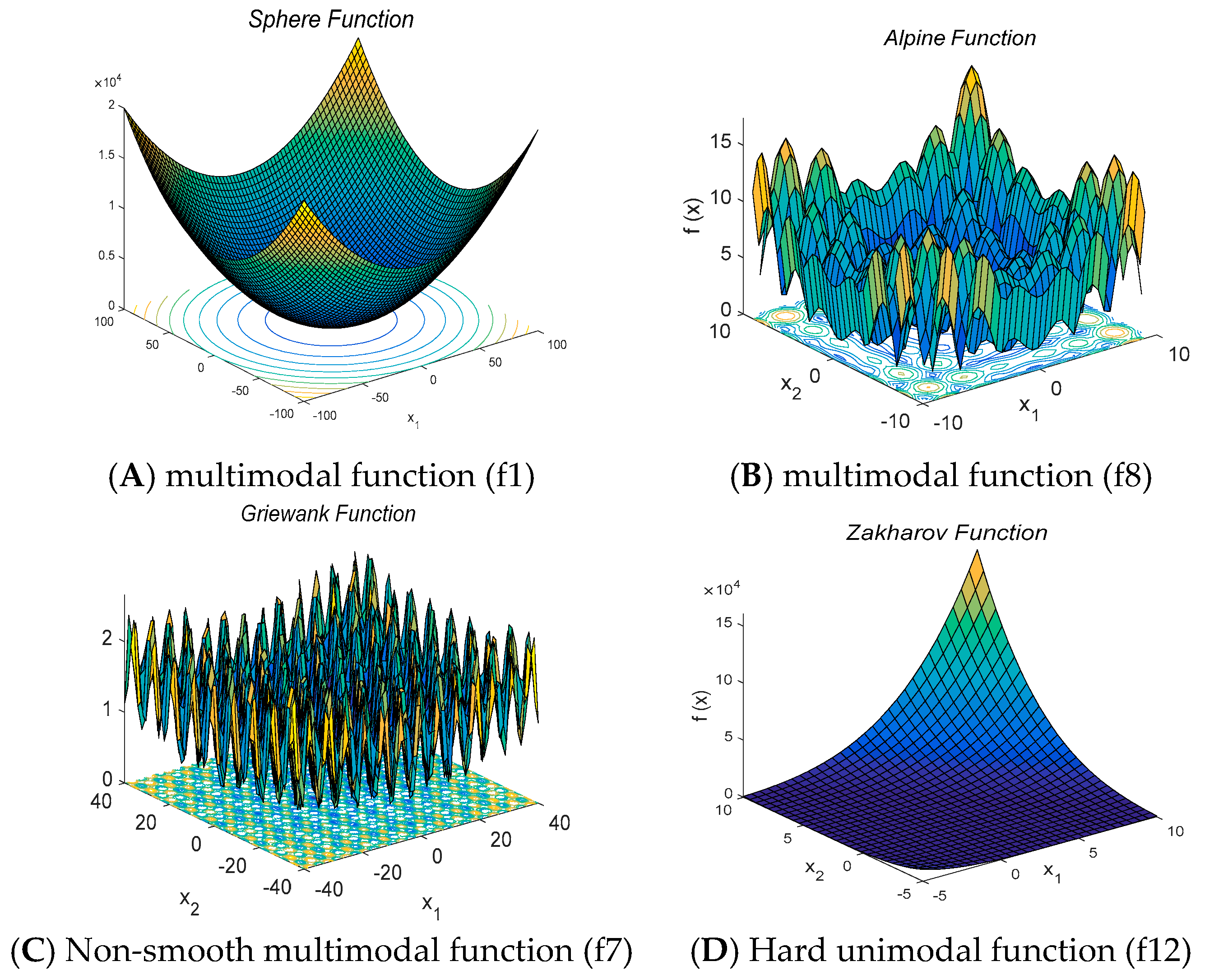
Figure 2.
Convergence speed for Sphere (f1) function (50D).

Figure 3.
Convergence speed for Griewank (f7) function (30D).

Figure 4.
Convergence speed for Cigar (f14) function (25D).
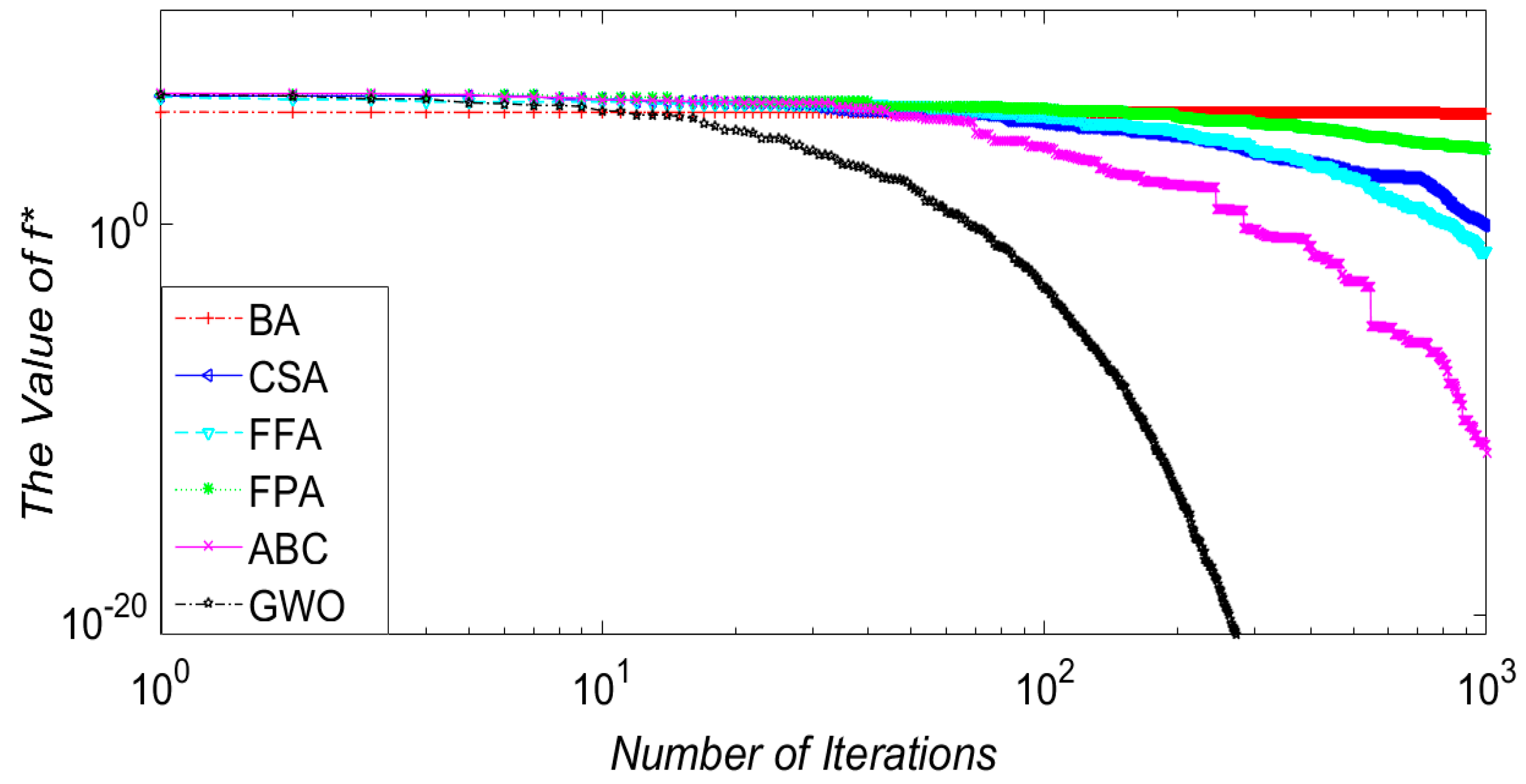
Figure 5.
Required Computation time by each method on a set of benchmark function.

Figure 6.
Impact of increasing number of function dimensions vs. CPU time for Sphere function.
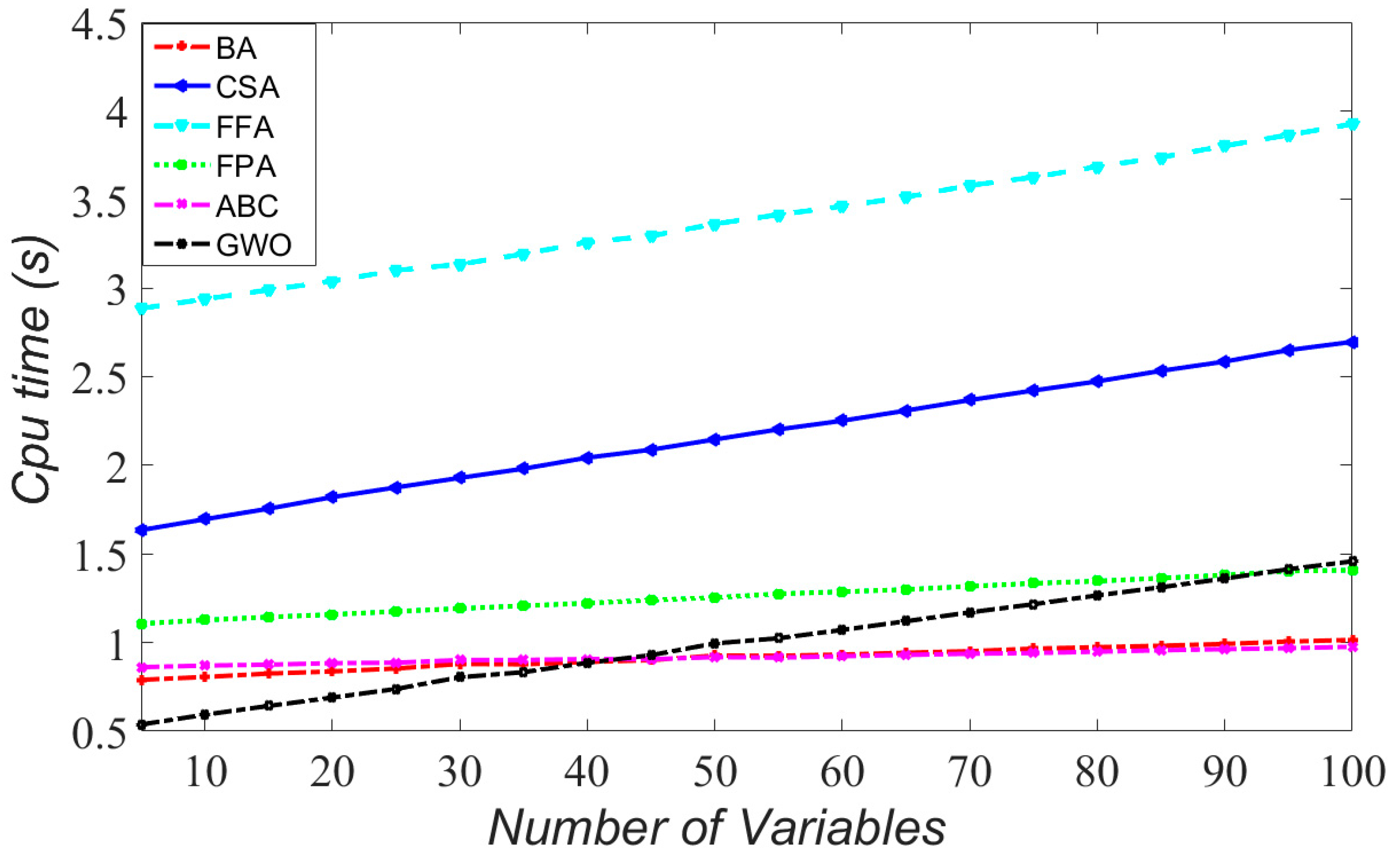
Figure 7.
Impact of increasing number of function dimensions vs. CPU time for Dixon and price function.
Figure 7.
Impact of increasing number of function dimensions vs. CPU time for Dixon and price function.
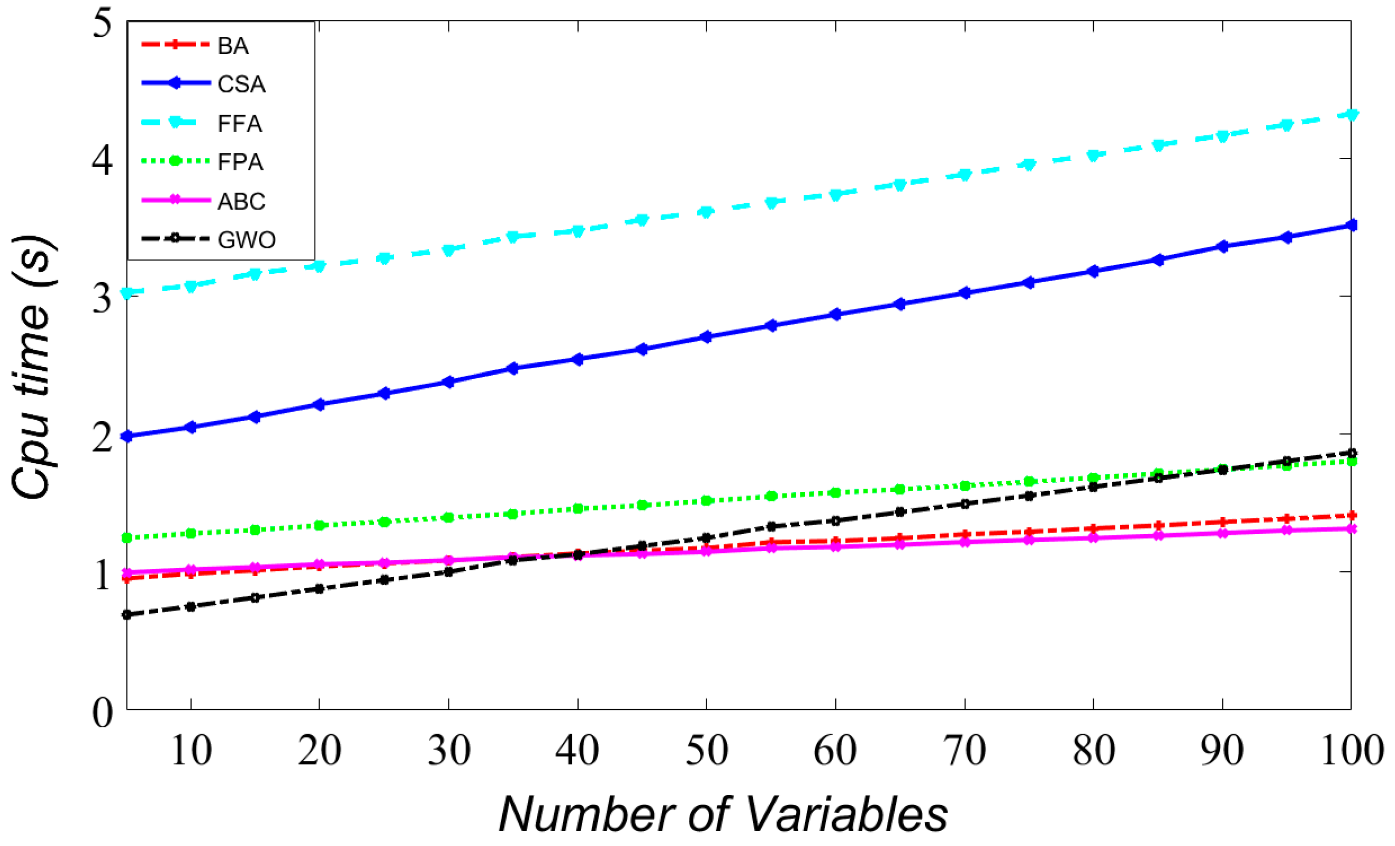
Figure 8.
Error vs. variable number for Sphere function.

Figure 9.
Error vs. variable number for Griewank function (f7).

Figure 10.
Error vs. variable number for Dixon and Price function (f13).
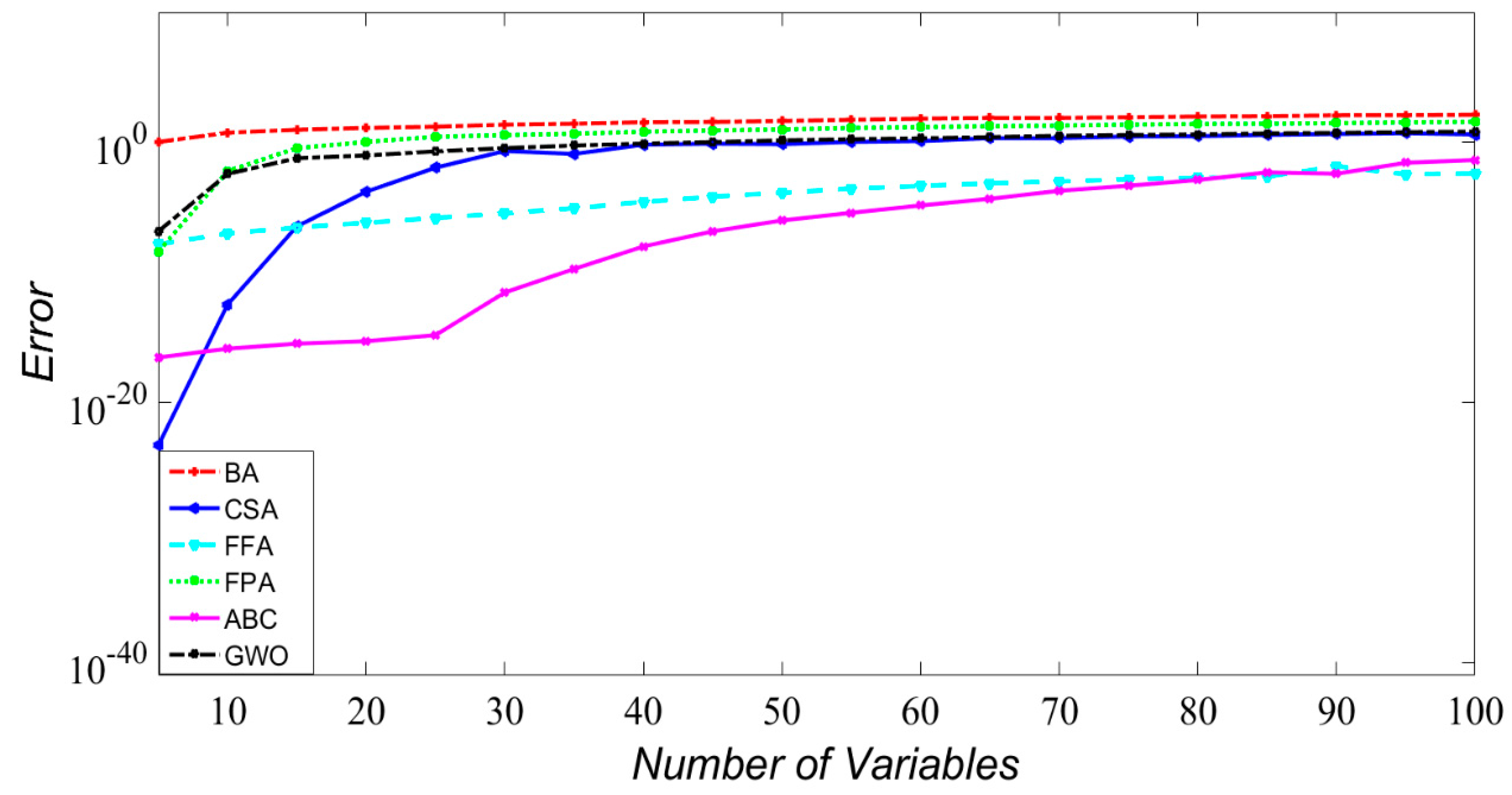
Figure 11.
The welded beam problem results.
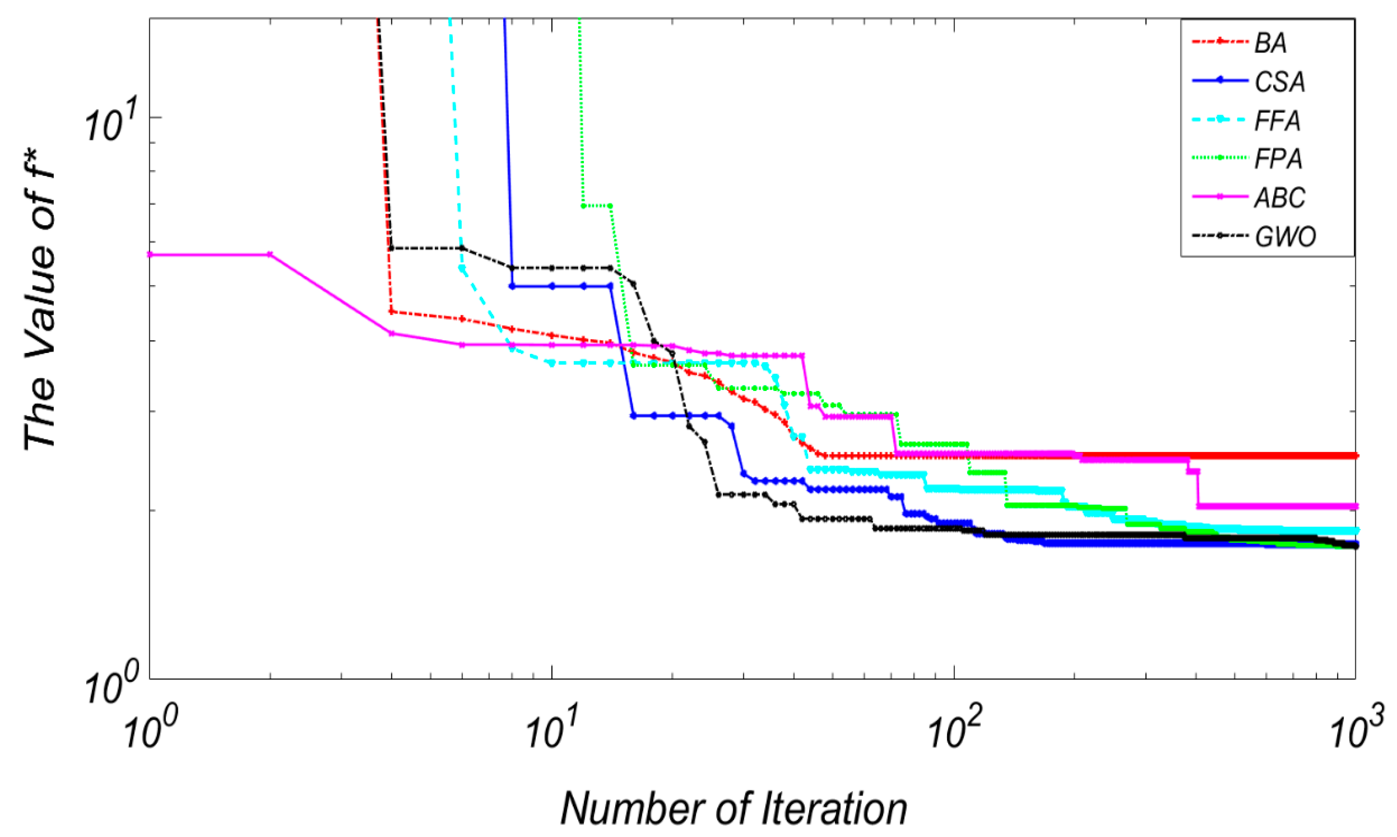
Figure 12.
The tension/compression spring problem results.

Figure 13.
Required CPU time by each algorithm for all constrained problems.
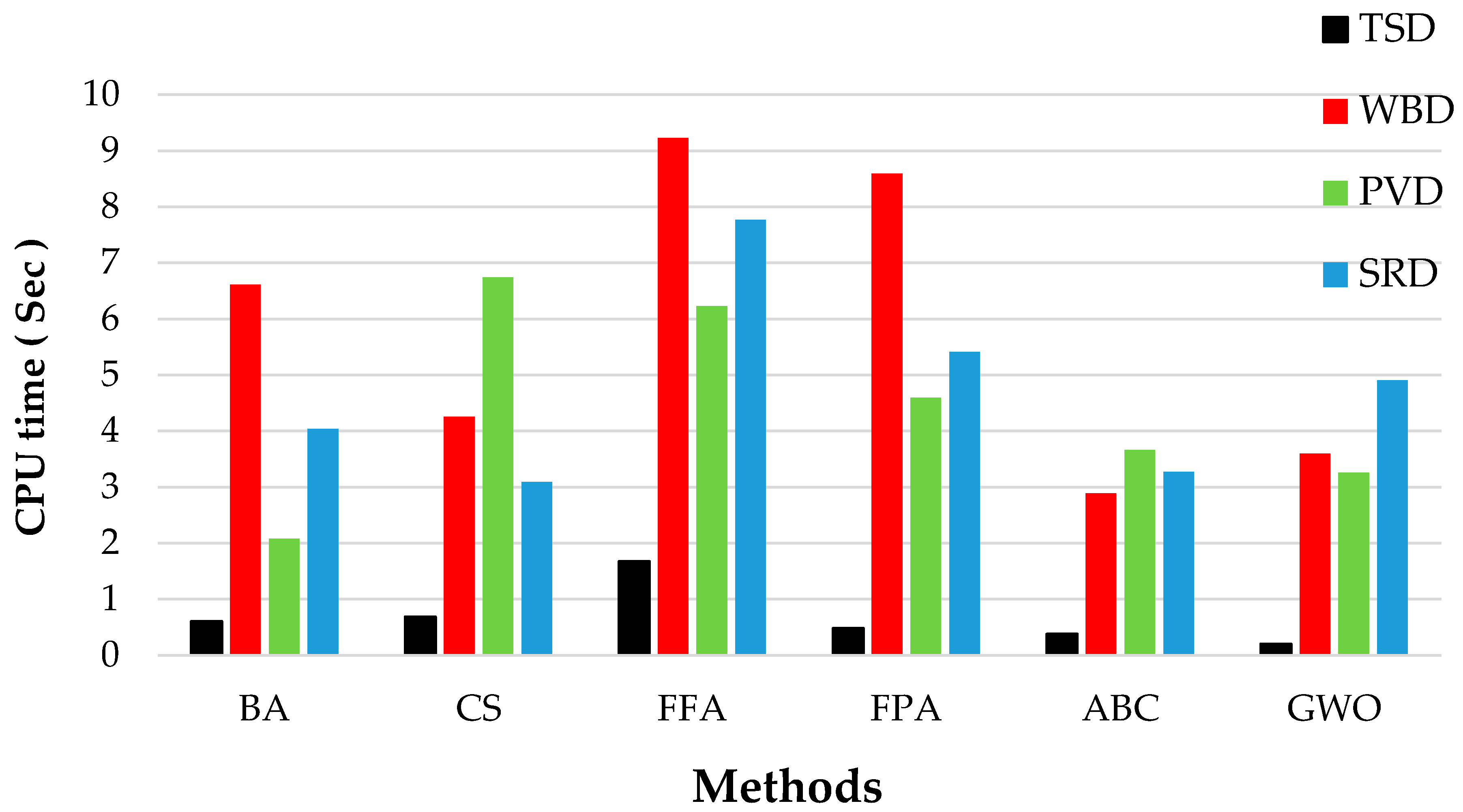
Figure 14.
Floating Offshore Wind Turbine (FOWT) with a spar buoy support structure.
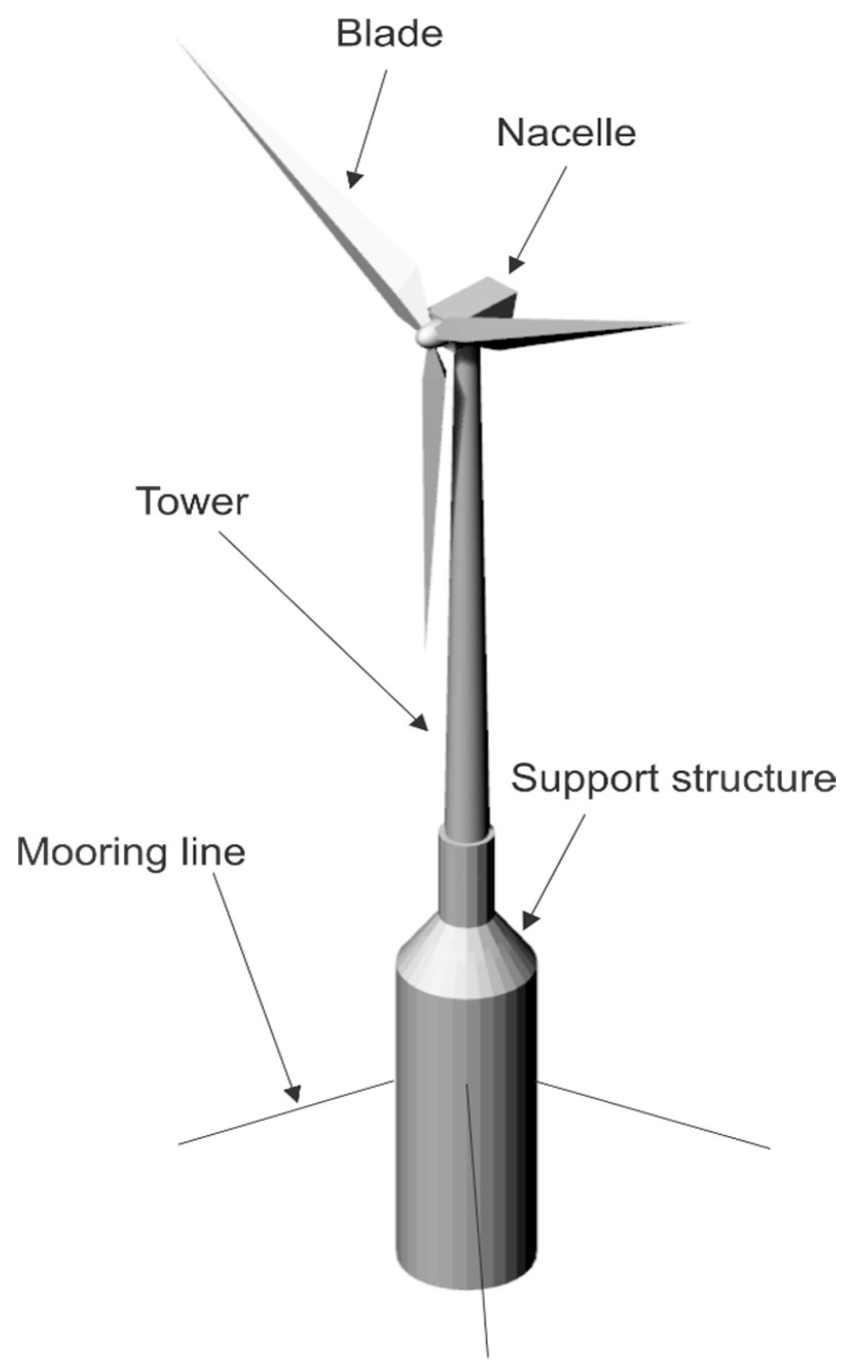
Figure 15.
Design characteristics of a spar buoy platform including height, radius, and taper ratio of the cylinder as well as platform’s free board.
Figure 15.
Design characteristics of a spar buoy platform including height, radius, and taper ratio of the cylinder as well as platform’s free board.

Figure 16.
Cost for FOWT problem results.
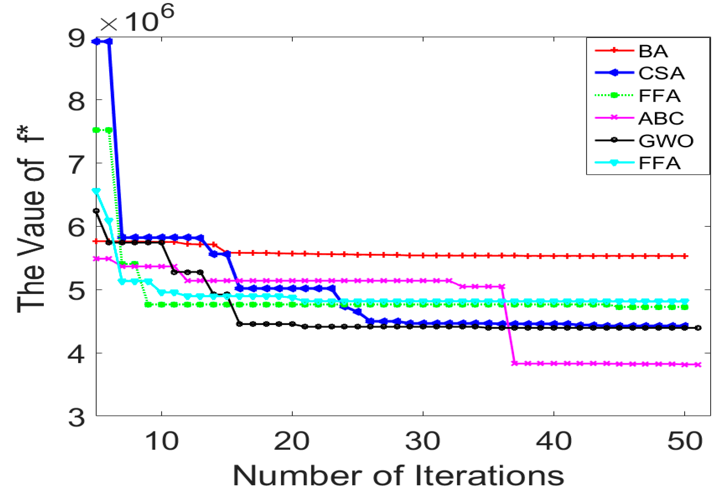
Figure 17.
Required CPU time for FOWT problem.
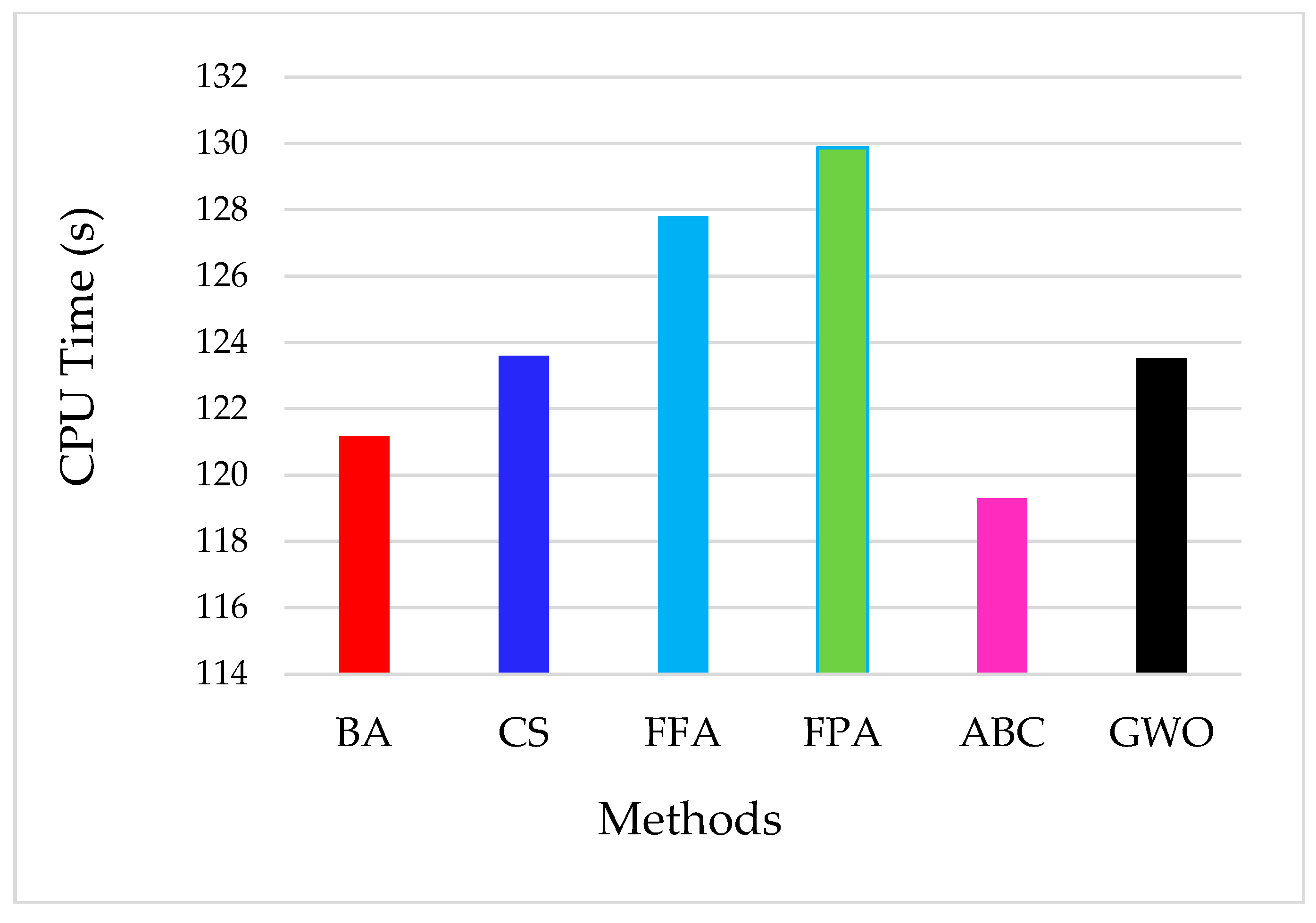

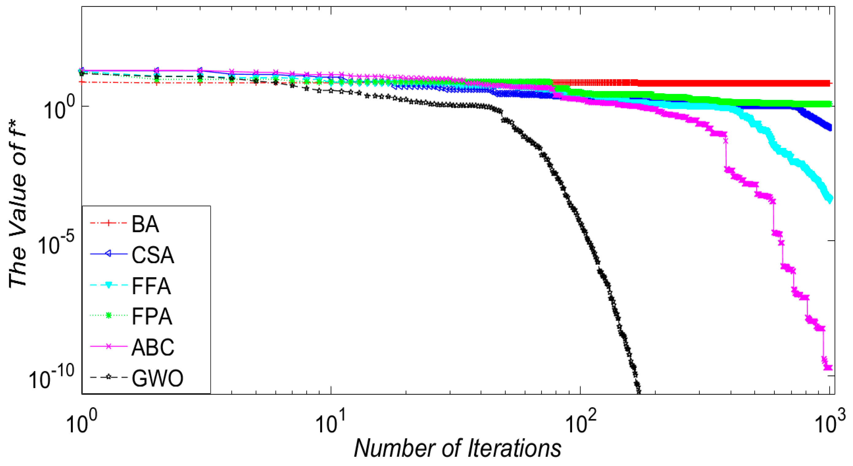
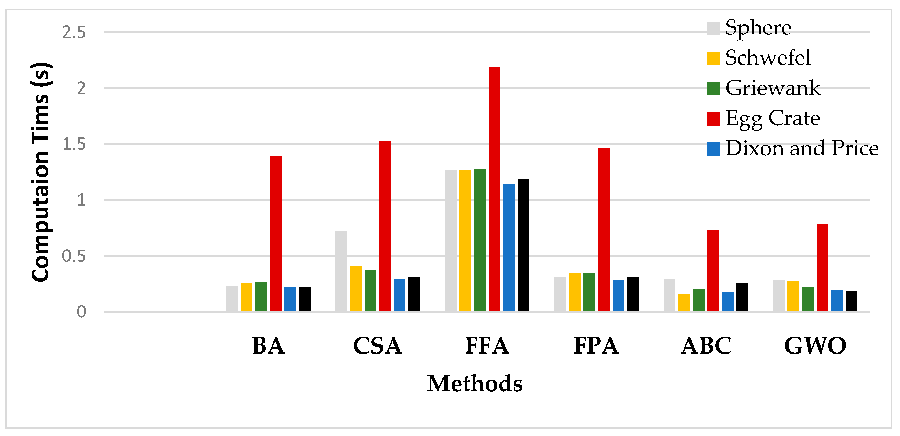
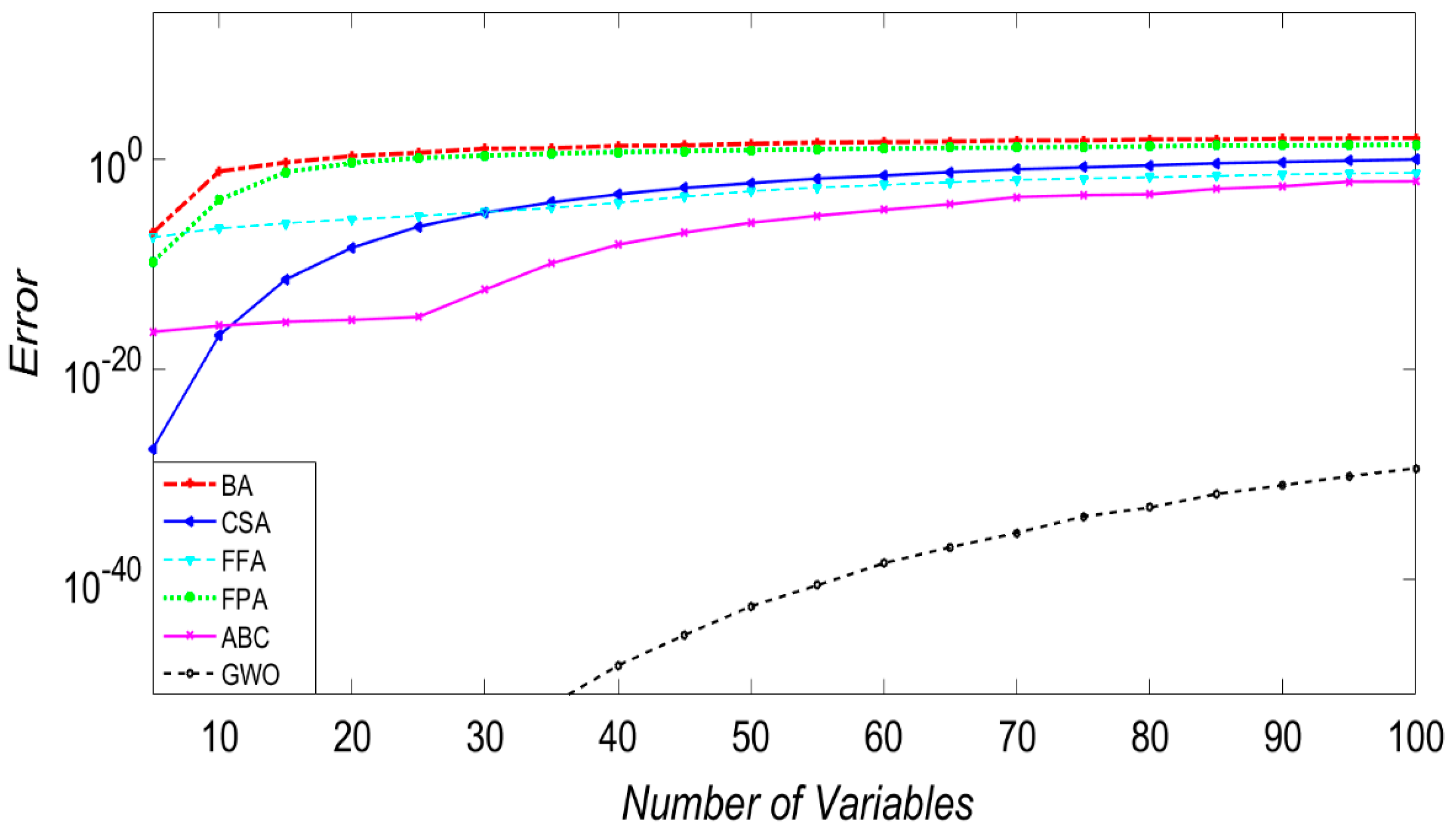
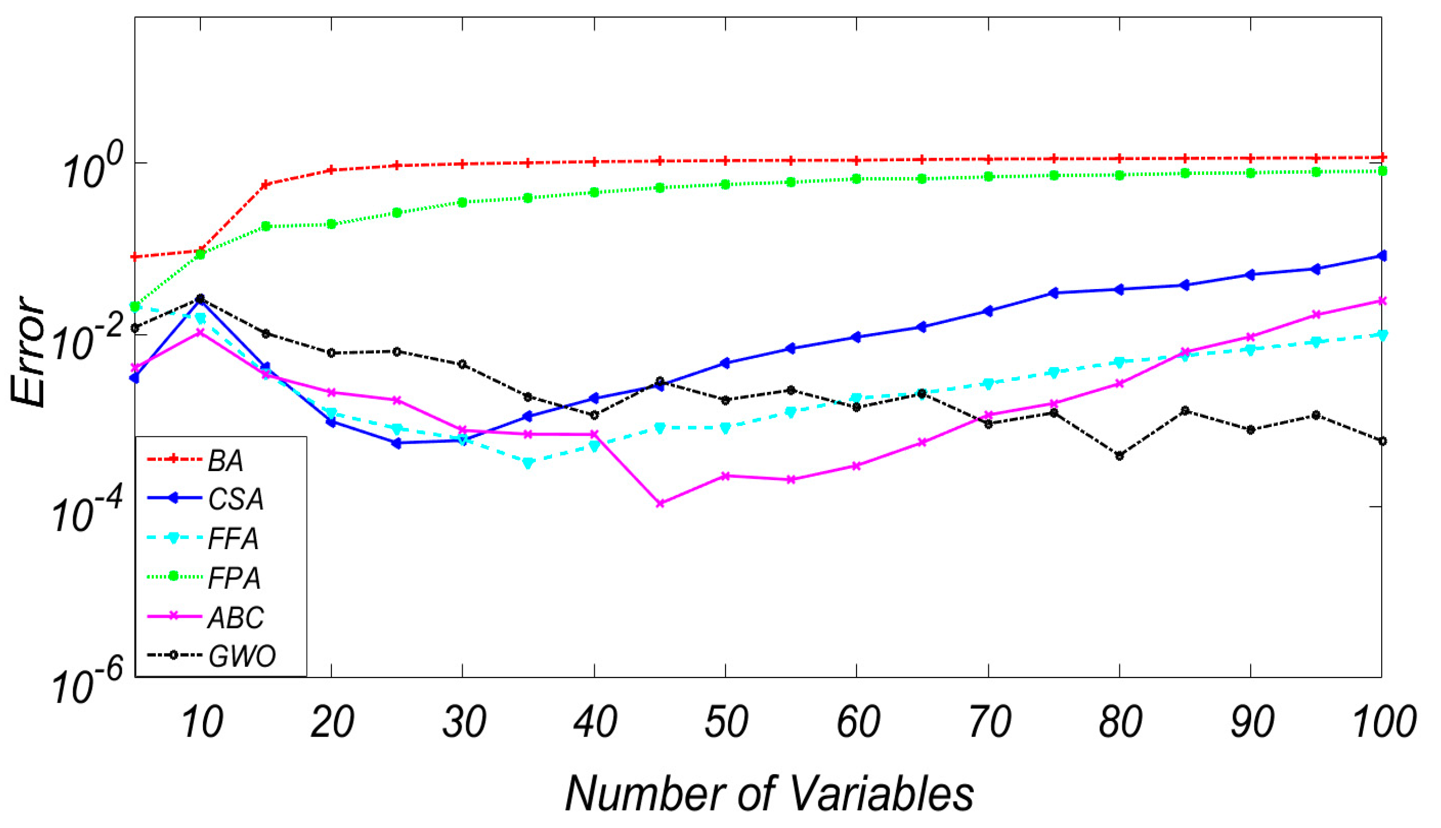
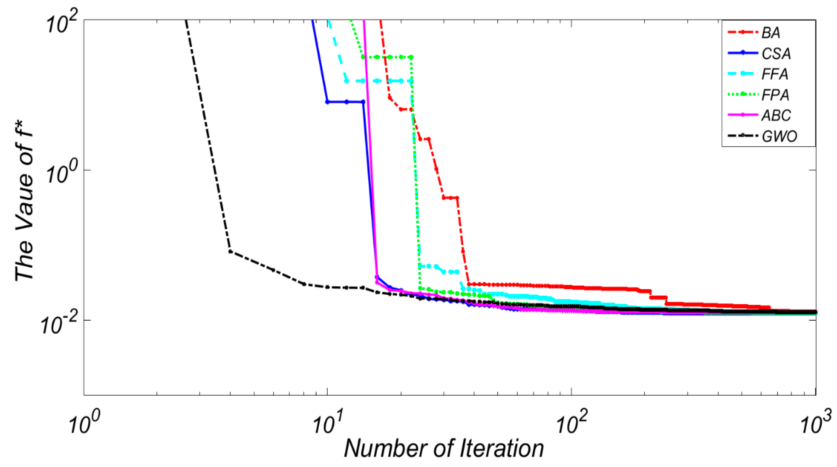
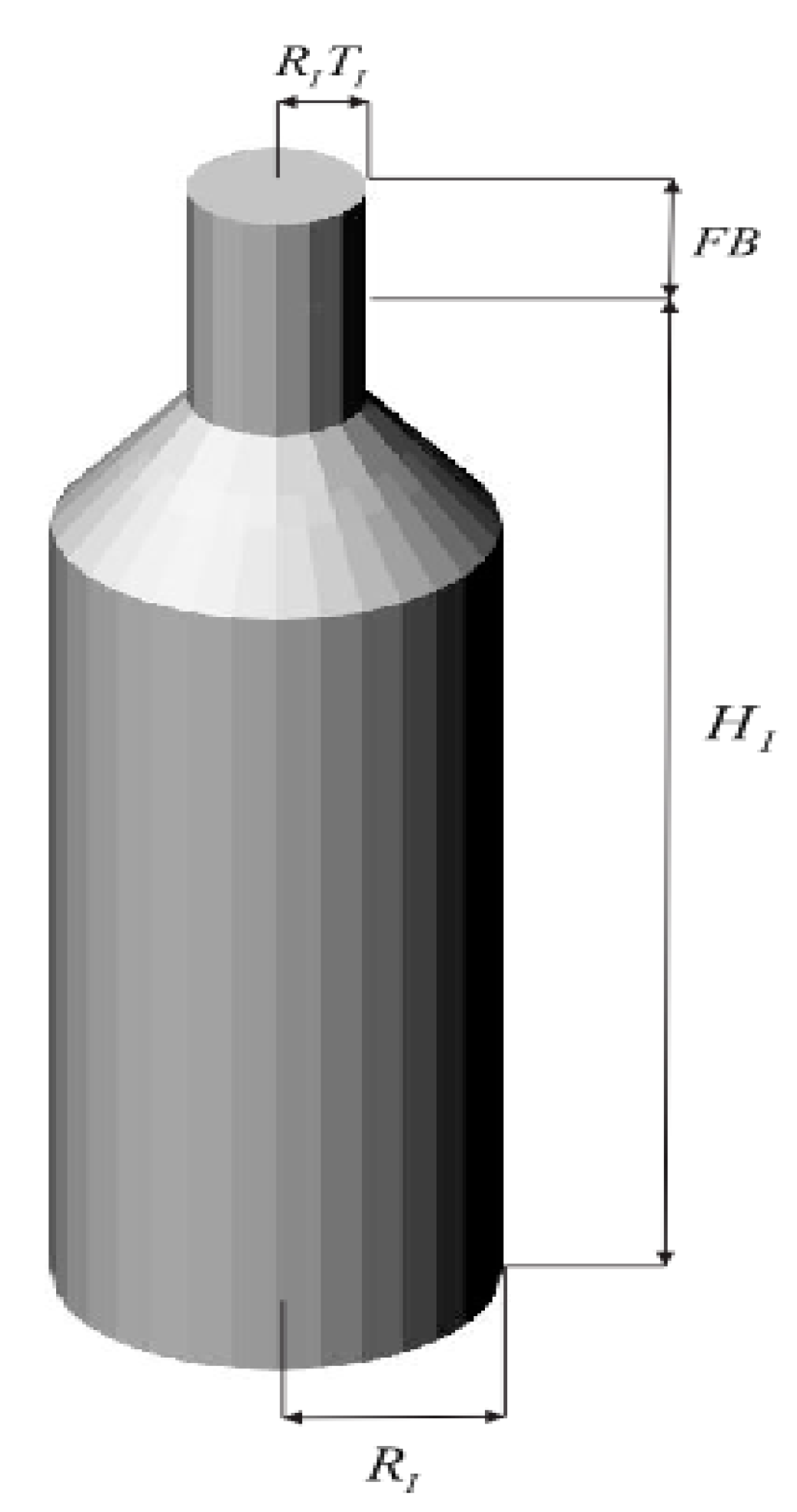
Table 1.
Symbols and Notations.
| Symbol | Description |
|---|---|
| NFE | Number of Function Evolution |
| D | Dimensional |
| CPU | Computation time |
| GO | Global Optimization |
| TSP | Travelling Salesman problem |
| Step size in CSA | |
| Scaling factor to control the step size in FFA | |
| Attractiveness of firefly in FFA | |
| Wavelengths in BA | |
| p | Switch probability |
| N | population size |
Table 2.
Selected benchmark functions.
| No | Function | Formula | f* | D | Space | Properties |
|---|---|---|---|---|---|---|
| f1 | Sphere | 0 | 50 | [−5.12 5.12]50 | Unimodal | |
| f2 | Sargan | 0 | 50 | [−100 100]50 | Unimodal | |
| f3 | S. Square | 0 | 50 | [−10 10]50 | Unimodal | |
| f4 | Powell | 0 | 50 | [−4 5]50 | Unimodal | |
| f5 | Schwefel | 0 | 50 | [−100 100]50 | Unimodal | |
| f6 | Ackley | 0 | 30 | [−32 32]30 | Multi-modal | |
| f7 | Griewank | 0 | 30 | [−100 100]30 | Multi-modal | |
| f8 | Alpine | 0 | 30 | [−10 10] | Multi-modal | |
| f9 | Egg Crate | 0 | 30 | [−5 5] | Multi-modal | |
| f10 | Rastrigin | 0 | 30 | [−10 10] | Multi-modal | |
| f11 | Leon | 0 | 25 | [−1.2 1.2] | Hard convergence unimodal | |
| f12 | Zakharov | 0 | 25 | [−5 10] | Hard convergence unimodal | |
| f13 | Dixon-Price | 0 | 25 | [−5 5] | Hard convergence unimodal | |
| f14 | Cigar | 0 | 25 | [−100 100] | Hard convergence multi-modal | |
| f15 | Levy | 0 | 25 | [−10 10] | Hard convergence multi-modal |
Table 3.
Setting parameters associated with each method.
| Algorithm | Setting Parameters |
|---|---|
| ABC | Food Source = 20, the limit value = 10 |
| FFA | = 0.5, = 1, = 1 |
| CSA | p = 0.25, |
| BA | Population Loudness (A) = 0.25, Pulse rate F [0, 2] |
| FPA | p = 0.8, = 1.5 |
| GWO | , C [0, 3] |
Table 4.
This table is a summary of results for unconstrained optimization problems.
| Alg. | f1 (D = 50) | f2 (D = 50) | f3 (D = 50) | ||||||||||||
| Min | Median | SD | NFE | CPU | Min | Median | SD | NFE | CPU | Min | Median | SD | NFE | CPU | |
| BA | 3.168 | 13.91 | ±8.94 | 20,000 | 0.219 | 79160 | 829400 | ±2.74 × 10 5 | 20,000 | 0.484 | 4242 | 5812 | ±210 | 20,000 | 0.234 |
| CSA | 0.6846 | 5.443 | ±35.09 | 20,000 | 0.375 | 14.06 | 2430 | ±1.72 × 10 5 | 20,000 | 1.219 | 1.5841 | 29.54 | ±237 | 20,000 | 0.719 |
| FFA | 1.1 × 10⁻³ | 0.1129 | ±38.27 | 20,000 | 1.266 | 0.1299 | 200.2 | ±2.16 × 10⁵ | 20,000 | 1.453 | 3.1861 | 13.67 | ±298 | 20,000 | 1.266 |
| FPA | 7.373 | 10.10 | ±35.66 | 20,000 | 0.344 | 187900 | 34570 | ±2.70 × 10⁵ | 20,000 | 0.547 | 1099 | 2518 | ±413 | 20,000 | 0.313 |
| ABC | 5.60 × 10⁻⁵ | 0.2723 | ±68.51 | 12,170 | 0.172 | 4.5 × 10⁻³ | 0.0321 | ±3.42 × 10² | 19,956 | 0.449 | 5.60 × 10⁵ | 16.18 | ±637 | 17,534 | 0.172 |
| GWO | 6.14 × 10−56 | 6.27 × 10⁻¹⁹ | ±20.60 | 20,000 | 0.297 | 0 | 4.76 × 10⁻¹⁹ | ±1.49 × 10⁵ | 20,000 | 0.469 | 0 | 4.20 × 10⁻²⁶ | ±175 | 20,000 | 0.281 |
| f4 (D = 50) | f5 (D = 50) | f6 (D = 30) | |||||||||||||
| Min | Median | SD | NFE | CPU | Min | Median | SD | NFE | CPU | Min | Median | SD | NFE | CPU | |
| BA | 11.92 | 147.1 | ±303.8 | 20,000 | 0.50 | 1.44 × 10⁻⁷ | 4.4 × 10⁻⁷ | ±0.177 | 20,000 | 0.234 | 16.77 | 16.77 | ±0.576 | 20,000 | 0.25 |
| CSA | 6.38 × 10⁻² | 1.094 | ±1792 | 20,000 | 1.109 | 5.03 × 10−43 | 9.51 × 10⁻²⁵ | ±0.052 | 20,000 | 0.406 | 4.567 | 6.99 | ±3.99 | 20,000 | 0.375 |
| FFA | 2.644 | 5.696 | ±1332 | 20,000 | 1.406 | 1.64 × 10⁻⁵ | 1.77 × 10⁻⁴ | ±0.078 | 20,000 | 1.266 | 1.30 × 10⁻³ | 9.61 × 10⁻² | ±1.51 | 20,000 | 1.234 |
| FPA | 54.89 | 109.7 | ±2759 | 20,000 | 0.578 | 0 | 2.17 × 10⁻¹³ | ±0.128 | 20,000 | 0.344 | 3.022 | 4.206 | ±4.268 | 20,000 | 0.313 |
| ABC | 5.10 × 10⁻³ | 0.631 | ±1356 | 20,096 | 0.297 | 3.12 × 10⁻⁴ | 3.45 × 10⁻² | ±0.755 | 20,005 | 0.156 | 5.79 × 10⁻⁵ | 9.34 × 10⁻² | ±4.36 | 19,645 | 0.188 |
| GWO | 1.23 × 10⁻⁶ | 1.10 × 10⁻³ | ±1190 | 20,000 | 0.453 | 0 | 0 | ±0.760 | 20,000 | 0.303 | 7.99 × 10⁻¹⁵ | 8.10 × 10⁻¹⁵ | ±2.43 | 20,000 | 0.203 |
| f7 (D = 30) | f8 (D = 30) | f9 (D = 30) | |||||||||||||
| Min | Median | SD | NFE | CPU | Min | Median | SD. | NFE | CPU | Min | Median | SD | NFE | CPU | |
| BA | 6.867 | 6.960 | ±0.173 | 20,000 | 0.266 | 2.53 × 10⁻⁷ | 3.04 × 10⁻⁶ | ±1.90 × 10⁻³ | 20,000 | 0.219 | 7.416 × 10⁻¹⁴ | 5.91 × 10 −12 | ±1.10 × 10⁻⁶ | 20,000 | 1.391 |
| CSA | 0.1534 | 1.073 | ±2.647 | 20,000 | 0.375 | 3.94 × 10⁻¹³ | 2.74 × 10⁻¹⁰ | ±2.80 × 10⁻⁴ | 20,000 | 0.375 | 1.346 × 10−75 | 1.70 × 10⁻³⁴ | ±0.166 | 20,000 | 1.531 |
| FFA | 3.21 × 10⁻⁴ | 0.2293 | ±1.922 | 20,000 | 1.281 | 5.57 × 10⁻⁹ | 1.31 × 10⁻⁶ | ±1.90 × 10⁻⁴ | 20,000 | 1.5 | 9.818 × 10⁻¹⁴ | 1.10 × 10⁻⁹ | ±0.062 | 20,000 | 2.188 |
| FPA | 1.1599 | 1.353 | ±1.455 | 20,000 | 0.328 | 3.43 × 10⁻¹⁰ | 3.08 × 10⁻⁸ | ±1.17 × 10⁻² | 20,000 | 0.344 | 1.06 × 10−36 | 1.30 × 10⁻²¹ | ±1.80 × 10⁻⁶ | 20,000 | 1.469 |
| ABC | 1.96 × 10⁻¹⁰ | 1.20 × 10⁻³ | ±3.159 | 16,890 | 0.203 | 5.50 × 10⁻⁶ | 5.50 × 10⁻⁶ | ±4.62 × 10⁻² | 18,006 | 0.188 | 5.00 × 10⁻⁸ | 1.90 × 10⁻⁵ | ±0.153 | 20,175 | 0.734 |
| GWO | 0 | 0 | ±0.996 | 20,000 | 0.234 | 0 | 0 | ±0.9112 | 20,000 | 0.219 | 0 | 0 | ±2.00 × 10⁻² | 20,000 | 0.984 |
| f10 (D = 30) | f11 (D = 25) | f12 (D = 25) | |||||||||||||
| Min | Median | SD | NFE | CPU | Min | Median | SD | NFE | CPU | Min | Median | SD | NFE | CPU | |
| BA | 117.4 | 117.4 | ±34.98 | 20,000 | 0.234 | 6.44 × 10⁻¹¹ | 6.45 × 10⁻¹¹ | ±4.50 × 10² | 20,000 | 0.281 | 40.45 | 69.48 | ±22.80 | 20,000 | 0.219 |
| CS | 33.28 | 48.59 | ±44.13 | 20,000 | 0.328 | 0 | 0 | ±8.80 × 10² | 20,000 | 0.391 | 7.844 | 31.57 | ±5.41 × 10⁷ | 20,000 | 0.313 |
| FFA | 21.89 | 24.42 | ±53.68 | 20,000 | 1.234 | 4.59 × 10⁻¹⁴ | 2.43 × 10⁻⁹ | ±7.10 × 10³ | 20,000 | 1.203 | 0.7202 | 3.704 | ±1.05 × 10⁵ | 20,000 | 1.125 |
| FPA | 62.22 | 94.78 | ±50.91 | 20,000 | 0.297 | 2.42 × 10⁻²⁸ | 8.57 × 10⁻¹⁹ | ±2.61 × 10² | 20,000 | 0.359 | 15.71 | 40.18 | ±1.26 × 10⁵ | 20,000 | 0.281 |
| ABC | 1.93 × 10⁻⁹ | 2.249 | ±3937 | 19,700 | 0.161 | 3.71 × 10⁻⁵ | 3.71 × 10⁻⁵ | ±0.776 | 18,765 | 0.219 | 105.9 | 133.4 | ±2.52 × 10⁷ | 16,742 | 0.166 |
| GWO | 0 | 0 | ±33.09 | 20,000 | 0.291 | 1.10 × 10⁻⁶ | 1.11 × 10⁻⁶ | ±7.90 × 10² | 20,000 | 0.217 | 3.85 × 10−38 | 2.20 × 10⁻¹⁸ | ±2.31 × 10⁷ | 20,000 | 0.154 |
| f13 (D = 25) | f14 (D = 25) | f15 (D = 25) | |||||||||||||
| Min | Median | SD | NFE | CPU | Min | Median | SD | NFE | CPU | Min | Median | SD | NFE | CPU | |
| BA | 286.64 | 12,600 | ±1.15 × 10⁴ | 20,000 | 0.219 | 49000 | 51900 | ±1.68 × 10⁴ | 20,000 | 0.344 | 8.881 | 23.88 | ±10.29 | 20,000 | 0.221 |
| CS | 4.9342 | 80.59 | ±3.84 × 10⁴ | 20,000 | 0.297 | 0.9062 | 460.3 | ±4.34 × 10⁵ | 20,000 | 0.469 | 2.05 × 10⁻⁵ | 0.226 | ±15.44 | 20,000 | 0.313 |
| FFA | 1.2766 | 1.095 | ±3.45 × 10⁴ | 20,000 | 1.094 | 3.91 × 10⁻² | 248.9 | ±3.79 × 10⁵ | 20,000 | 1.734 | 7.86 × 10⁻⁷ | 3.30 × 10⁻³ | ±11.21 | 20,000 | 1.188 |
| FPA | 52.5473 | 314.1 | ±4.57 × 10⁴ | 20,000 | 0.281 | 7490 | 47800 | ±6.07 × 10⁵ | 20,000 | 0.406 | 2.977 | 6.616 | ±18.71 | 20,000 | 0.313 |
| ABC | 9.84 × 10⁻⁴ | 3.10 × 10⁻³ | ±1.53 × 10³ | 18,900 | 0.188 | 2.14 × 10⁻¹² | 1.20 × 10⁻³ | ±4.98 × 10⁵ | 19,150 | 0.25 | 1.436 × 10⁻¹⁵ | 1.3 × 10⁻⁶ | ±19.96 | 19,406 | 0.256 |
| GWO | 0.6666 | 2.70 × 10⁻³ | ±1.10 × 10³ | 20,000 | 0.172 | 0 | 5.05 × 10−45 | ±2.41 × 10⁵ | 20,000 | 0.234 | 0.1418 | 0.1804 | ±6.38 | 20,000 | 0.188 |
Table 5.
This table is a summary of results for nonlinear constrained engineering applications.
| Methods | Prob. | Analytical | ||||||||||
|---|---|---|---|---|---|---|---|---|---|---|---|---|
| f* | x1 | x2 | x3 | x4 | x5 | x6 | x7 | Obtained f* | NFE | CPU Time | ||
| BA | TSD | 0.012665 | 0.05123 | 0.34582 | 13.5571 | - | 0.013242 | 20,000 | 0.6078 | |||
| WBD | 1.738522 | 0.31623 | 5.5111 | 6.4044 | 0.49061 | - | - | -- | 1.8268 | 20,000 | 6.6091 | |
| PVD | 6059.71433 | 1.04938 | 0.51773 | 49.5176 | 187.5231 | - | - | - | 6190.4687 | 20,000 | 2.0781 | |
| SRD | 2996.34816 | 3.5 | 0.7 | 17 | 7.56 | 7.6892 | 3.5424 | 5.2458 | 3019.5833 | 20,000 | 4.0369 | |
| CS | TSD | 0.012665 | 0.05178 | 0.359011 | 11.1579 | - | - | - | - | 0.01266 | 20,000 | 0.6875 |
| WBD | 1.724852 | 0.20573 | 3.4705 | 9.0366 | 0.20573 | - | - | - | 1.7449 | 20,000 | 4.2563 | |
| PVD | 6059.71433 | 0.77714 | 0.384442 | 40.44869 | 178.2513 | - | - | - | 6074.587 | 20,000 | 6.7438 | |
| SRD | 2996.34816 | 3.5001 | 0.7032 | 17.1 | 7.4 | 7.80 | 3.46 | 5.27 | 3000.9597 | 20,000 | 3.0927 | |
| FFA | TSD | 0.012665 | 0.052209 | 0.370468 | 10.821 | - | - | - | - | 0.012713 | 20,000 | 1.675 |
| WBD | 1.727852 | 0.19588 | 3.7176 | 9.0367 | 0.20573 | - | - | - | 1.7291 | 20,000 | 9.2266 | |
| PVD | 6059.71433 | 0.902631 | 0.445717 | 46.92328 | 177.7547 | - | - | - | 6026.3068 | 20,000 | 6.225 | |
| SRD | 2996.34816 | 3.5 | 0.7 | 17 | 7.31 | 7.820 | 3.351 | 5.327 | 2996.3478 | 20,000 | 7.771 | |
| FPA | TSD | 0.012665 | 0.051643 | 0.35558 | 11.3619 | - | - | - | - | 0.012669 | 20,000 | 0.4843 |
| WBD | 1.724852 | 0.20573 | 3.4705 | 9.0366 | 0.20573 | - | - | - | 1.7568 | 20,000 | 8.5938 | |
| PVD | 6059.71433 | 0.77447 | 0.38323 | 40.32289 | 179.959 | - | - | - | 5990.4928 | 20,000 | 4.5969 | |
| SRD | 2996.34816 | 3.5 | 0.761 | 17.001 | 7.1 | 7.54 | 3.3521 | 5.3412 | 3019.5833 | 20,000 | 5.4109 | |
| ABC | TSD | 0.012665 | 0.052855 | 0.37997 | 10.1552 | - | - | - | - | 0.012657 | 16,092 | 0.3796 |
| WBD | 1.729852 | 0.20866 | 3.3293 | 8.9139 | 0.20453 | - | - | - | 1.7251 | 17,145 | 6.8906 | |
| PVD | 6059.71433 | 0.84036 | 0.426735 | 42.56989 | 176.4665 | - | - | - | 6059.037 | 16,200 | 3.6609 | |
| SRD | 2996.34816 | 3.512 | 0.7 | 17 | 7.3 | 7.8 | 3.3502 | 5.2866 | 2996.3088 | 18,700 | 3.2701 | |
| GWO | TSD | 0.012665 | 0.051149 | 0.305127 | 10.7273 | - | - | - | - | 0.012665 | 20,000 | 0.2031 |
| WBD | 1.724852 | 0.20431 | 3.5018 | 9.0378 | 0.20576 | - | - | - | 1.7266 | 20,000 | 6.5938 | |
| PVD | 6059.71433 | 0.8125 | 0.434511 | 42.0891 | 176.7587 | - | - | - | 6059.7639 | 20,000 | 3.2563 | |
| SRD | 2996.34816 | 3.46427 | 0.7129 | 17.1001 | 7.25581 | 7.18738 | 3.2359 | 5.7814 | 3005.6092 | 20,000 | 4.9021 | |
Table 6.
Geometric design variables of spar buoy platform.
| Variable | Description | Min. | Max. |
|---|---|---|---|
| HI | Central cylinder draft | 2 m | 150 m |
| RI | Central cylinder radius | 3 m | 25 m |
| TI | Top tapper ratio | 0.2 | 2 |
| XM | Mooring System | 0.2 | 2 |
Table 7.
Summary of comparison result for support structure cost for FOWTs application.
| Methods | f* Min | NFE | CPU Time |
|---|---|---|---|
| BA | 5,533,111.9378 | 1000 | 121.1719 |
| CSA | 4,426,006.2921 | 1000 | 123.5938 |
| FFA | 4,811,655.8121 | 1000 | 131.8125 |
| FPA | 4,727,085.732 | 1000 | 132.875 |
| ABC | 3,817,499.5279 | 951 | 119.2969 |
| GWO | 4,395,036.2793 | 1000 | 123.5313 |
© 2017 by the authors. Licensee MDPI, Basel, Switzerland. This article is an open access article distributed under the terms and conditions of the Creative Commons Attribution (CC BY) license (http://creativecommons.org/licenses/by/4.0/).
Share and Cite
MDPI and ACS Style
Saad, A.E.H.; Dong, Z.; Karimi, M. A Comparative Study on Recently-Introduced Nature-Based Global Optimization Methods in Complex Mechanical System Design. Algorithms 2017, 10, 120. https://doi.org/10.3390/a10040120
AMA Style
Saad AEH, Dong Z, Karimi M. A Comparative Study on Recently-Introduced Nature-Based Global Optimization Methods in Complex Mechanical System Design. Algorithms. 2017; 10(4):120. https://doi.org/10.3390/a10040120
Chicago/Turabian StyleSaad, Abdulbaset El Hadi, Zuomin Dong, and Meysam Karimi. 2017. "A Comparative Study on Recently-Introduced Nature-Based Global Optimization Methods in Complex Mechanical System Design" Algorithms 10, no. 4: 120. https://doi.org/10.3390/a10040120
Note that from the first issue of 2016, this journal uses article numbers instead of page numbers. See further details here.