Scheduling Non-Preemptible Jobs to Minimize Peak Demand


1
Los Alamos National Laboratoy, Los Alamos, NM 87545, USA
2
Gianforte School of Computing, Montana State University, Bozeman, MT 59717,USA
*
Author to whom correspondence should be addressed.
Algorithms 2017, 10(4), 122; https://doi.org/10.3390/a10040122
Submission received: 22 September 2017
/
Revised: 20 October 2017
/
Accepted: 25 October 2017
/
Published: 28 October 2017
(This article belongs to the Special Issue Algorithms for Hard Problems: Approximation and Parameterization)
Abstract
:This paper examines an important problem in smart grid energy scheduling; peaks in power demand are proportionally more expensive to generate and provision for. The issue is exacerbated in local microgrids that do not benefit from the aggregate smoothing experienced by large grids. Demand-side scheduling can reduce these peaks by taking advantage of the fact that there is often flexibility in job start times. We focus attention on the case where the jobs are non-preemptible, meaning once started, they run to completion. The associated optimization problem is called the peak demand minimization problem, and has been previously shown to be NP-hard. Our results include an optimal fixed-parameter tractable algorithm, a polynomial-time approximation algorithm, as well as an effective heuristic that can also be used in an online setting of the problem. Simulation results show that these methods can reduce peak demand by up to 50% versus on-demand scheduling for household power jobs.
1. Introduction
The problem of scheduling non-preemptible jobs occurs naturally in smart power grid systems, in which communication can occur between energy consumers and the energy provider. Some household appliances require instant functionality (e.g., light bulbs), but many others have more flexibility in exactly when they operate (e.g., dishwasher or water heater). Peaks in power demand are proportionally more expensive to generate and provision for (since more infrastructure is required), so it is advantageous to schedule power-consuming jobs in such a way as to minimize peak demand. This problem has been previously formalized as the Peak demand minimization (PDM) problem, and has been studied extensively [1,2,3,4,5,6,7,8]. The basic formulation of the problem is as follows: Each job j is non-preemptible, meaning once it begins execution, it must run to completion without any interruptions. Each job j is characterized by four parameters: an arrival time (), deadline (), and length () that are real-valued for continuous timescales and integer-valued for discrete timescales, and a real-valued instantaneous demand () which is conceptually the height of the job. The arrival time and deadline are within the fixed time interval and form the execution window of the job. Job j is scheduled by assigning it a start time, , which allows it to run in the closed interval such that . The demand at time t is the sum of the job heights that are scheduled to run during t:
Then, the peak demand, , of the schedule is the maximum demand for any time t in ,
The PDM problem is to determine a job schedule, , that minimizes . In this work, we propose three algorithms to solve PDM:
- An optimal dynamic programming algorithm for discrete-timescale instances that utilizes branch-and-bound techniques that is fixed-parameter tractable.
- A polynomial-time randomized algorithm based on linear programming that provides an -approximation, where n is the number of jobs, and is the first known approximation for PDM.
- An effective and simple heuristic algorithm that can be used in either an online or offline fashion.
2. Related Work
Many variations on modifying demand to improve the efficiency of power grids (generically called demand response) have been explored. These approaches can generically be categorized as utility function optimization (commonly cost function minimization) and peak demand minimization (PDM). Utility function optimization techniques use price incentives to encourage consumers to modify their behavior, and are outside the scope of this work.
PDM aims to directly schedule jobs to reduce peaks in power schedules instead of passively influencing changes with price incentives. PDM has been studied in the context of preemptible jobs (i.e., jobs that can be interrupted partway through execution) [1,2]. In this paper, we consider the scenario where jobs are non-preemptible, and thus must run to completion once started. The PDM problem has been found to be NP-hard to approximate within a ratio of 2 in this scenario [3]. Heuristics have been developed that show promise in practice, but which provide no theoretical guarantee [4,5]. Approximation algorithms have been developed for the special case where all jobs have the same start time and deadline [6,7]. Our work introduces the first general purpose approximation algorithm where no assumptions are placed on the job parameters. Finally, optimal algorithms have been introduced that work on a limited number of jobs [3,8]. Our work also introduces an optimal fixed-parameter tractable algorithm that is able to schedule approximately 15 times more jobs in practice than previous approaches.
Non-preemptible power job scheduling is also similar to the machine minimization problem and rectangular strip packing [9,10,11,12,13]. In the machine minimization problem, jobs are assumed to have unit height, as opposed to power jobs that can have variable height. The main differences with rectangular strip packing are that in the general PDM case, jobs are limited in where they can be placed in the strip, and once jobs are scheduled, they do not need to remain as intact rectangles. Since job height represents the power required, each segment of a scheduled job will drop to lie on top of the job below it, instead of remaining as an intact rectangle in the strip.
3. Algorithms
We first present an optimal fixed-parameter tractable algorithm that improves on the efficiency of the method described in [3] due to an effective branch-and-bound idea. The second algorithm described is based on linear programming relaxation and randomized rounding that is a -approximation algorithm for the general PDM problem. Finally, we describe a heuristic approach that can also be adapted to the online setting of the problem.
3.1. An Optimal Dynamic Programming Algorithm
In this section, we detail a dynamic programming algorithm for PDM, inspired by the algorithm presented in [3]. Our algorithm takes a similar approach of identifying groups of overlapping jobs, but uses a tree-based schedule representation and a branch-and-bound strategy to reduce the search space, resulting in substantially better performance (able to run instances with 15 times as many jobs). We term this algorithm OptimalDP in the results section.
At a high level, the algorithm proceeds by first ordering jobs by increasing deadlines. For each job, every possible configuration of start times of that job and as well as other earlier jobs that could overlap it is considered. Job configurations are represented using trees, where each level in the tree represents the scheduling choices of one job. Pointers from leaf configurations of the current job to compatible configurations of the previous job are used to move between trees and generate a complete schedule for all jobs. Valid schedules can be built by traversing these trees backwards, beginning with a leaf node of the final job. A branch-and-bound approach is employed to limit unnecessary schedule exploration.
3.1.1. Configuration Lists
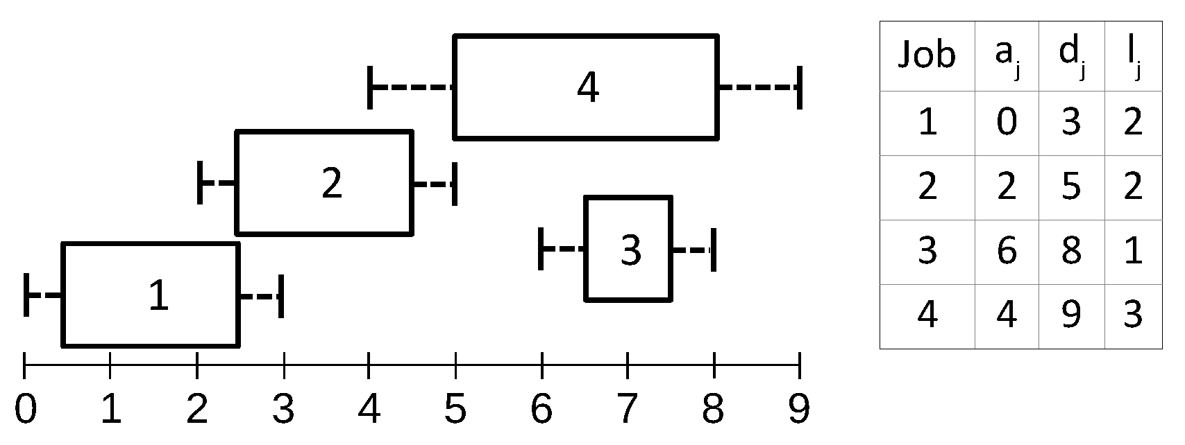
Jobs are sorted first by increasing deadline and then by increasing arrival time. For each job j, a list of preceding jobs —called the configuration list—is defined as the set of jobs whose execution windows either overlap j’s execution window, or overlap the execution window of a job following j. Figure 1 illustrates a sample set of jobs along with their configuration lists. We observe that each job configuration list consists of a consecutive interval in the sorted list of jobs; i.e., , where the head of each list has the earliest deadline (and arrival in case of ties).
Lemma 1.
The list heads are non-decreasing; i.e., .
Proof.
Suppose job . Since , . If , then since and . Thus . If , then and so . ☐
3.1.2. Configuration Trees
For each job j, we represent all possible configurations of start times of all the jobs in its configuration list using a configuration tree, . We consider these jobs in reverse order starting from j and create a branching tree, where nodes at level k in the tree correspond to the possible starting times for job (we assume the root of the tree is at level 0). Thus, each leaf l in provides a schedule of start times for all jobs in . Let be the peak demand of this particular schedule for the jobs in .
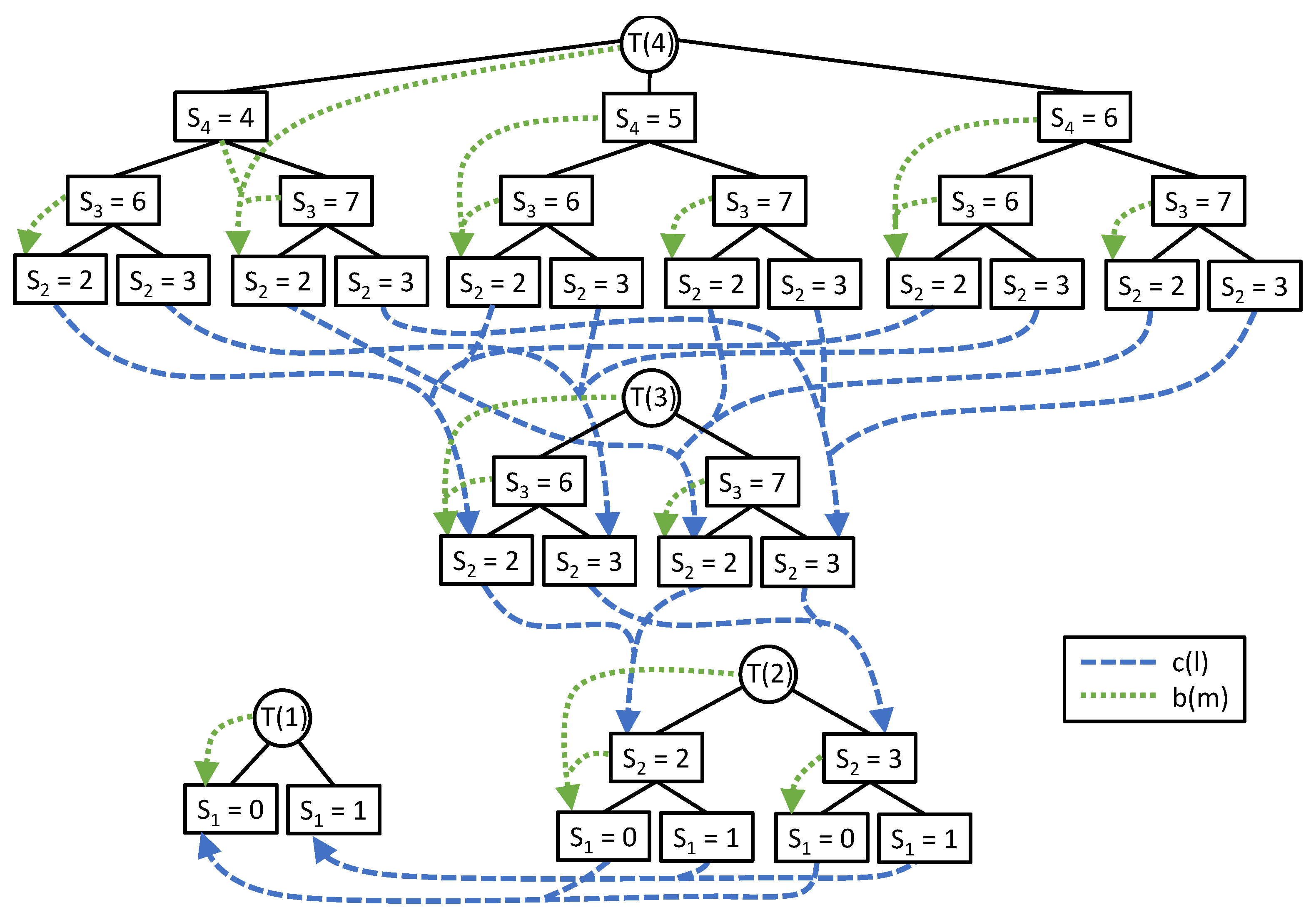
We need to keep track of compatible job configurations in order to build a consistent schedule for all jobs. We do this by maintaining a compatibility pointer, , from each leaf node l in to a compatible node in (). By Lemma 1, . Thus, we can follow the same path in that we took beginning with a node at level 2 in to reach the compatible node in . If , then we simply make each leaf in point to the root of . Note that compatibility pointers are stored only at the leaf nodes of trees . Figure 2 shows an example with four configuration trees.
3.1.3. Dynamic Programming
Once the configuration trees are constructed and compatibility pointers found, the minimum overall schedule can be found using dynamic programming, as follows:
For each leaf node , we compute , which is the peak height of an optimal schedule for jobs that is compatible with the configuration represented by l. For each node we will store a pointer, , to the leftmost leaf l in the subtree rooted at m with best (i.e., lowest) peak height . The pointer for a leaf node is to itself. The h values satisfy the following recurrence:
We note that once the values are found for a given tree , it is easy to compute the pointers for the internal nodes in a bottom-up fashion. Thus, we can apply dynamic programming to find the h and b values for each job configuration tree in order, beginning with . An optimal schedule can be found by following alternating b and c pointers, starting with . The peak height of this schedule will be given by (the b pointers are also shown in Figure 2).
3.1.4. Branch-and-Bound Approach
To avoid unnecessary tree expansion, a branch-and-bound technique can be employed to avoid explicitly building and storing configuration trees. Configuration lists are created for each job as described above. The algorithm keeps track of the peak demand for the best schedule found so far (initialized to ).
The algorithm begins a recursive process of building and exploring paths through the configuration trees by starting with the last job in the list. It proceeds in a depth-first fashion, creating subtrees of the previous job as compatibility pointers are followed. Once a new path has been established from the last job through the first, if a better solution is found, is updated. The search continues recursively to explore alternate paths. If at any point the current path creates a node m with , then that node can be marked as unnecessary to explore further and the search pruned.
3.1.5. Fixed-Parameter Tractability
An algorithm is said to be fixed-parameter tractable with respect to parameters of the input or output if the running time of the algorithm is a polynomial function of the input size times some function of the parameters: . The complexity of the algorithm is driven by the size of the configuration trees, , that can be bounded by their branching factor and maximum depth. The maximum branching factor is , and the maximum depth is . The following lemma shows that r is also a simple parameter of the input.
Lemma 2.
r is the maximum number of earlier jobs that overlap any job; i.e., .
Proof.
Let . Then . If for some , then this contradicts the choice of (since would contain , and so be a larger set). Thus and so . Since for all j, . It follows that . ☐
The maximum number of nodes in each configuration tree is . Since the dynamic programming time is easily seen to be linear in the size of the trees, the total running time is .
3.2. An Approximation Algorithm
In this section we detail a novel algorithm for the PDM problem that provides the first known approximation guarantee for the general PDM problem. The algorithm is based on relaxing an integer linear program (ILP) to allow real-valued solutions and then rounding the real-valued solution back to an integer solution.
3.2.1. Integer Linear Programming Formulation
The PDM problem can be formulated as an ILP using the following notation and variables:
- J—Set of jobs.
- —A finite set of valid execution intervals for job (an interval is valid for job j if and only if and ).
- —Height of job j.
- L—Set of all left hand time points of intervals in .
- —Peak demand.
- —Indicates if interval is scheduled.
The ILP is:
subject to:
Constraint (2) ensures that exactly one interval will be selected for each job, and (3) ensures that will denote the peak height of the schedule. Only elements of L need to be considered in (3) as a consequence of Lemma 3.
Lemma 3.
The maximum height of any schedule must occur for some .
Proof.
Schedule height only increases at the moment a new job begins processing, and thus the peak height of a schedule must be initiated at the start time of some job. Since L is the collection of all possible start times for all jobs, some point in L must correspond to the arrival time of the peak height of the schedule. ☐
3.2.2. A Randomized Rounding Algorithm
The ILP presented above cannot be efficiently solved due to the restriction of to integer values. To address this, we construct a relaxed LP in the exact same fashion as the ILP, except the variables may take on any values in the range . After the relaxed LP is solved, a specific interval is selected for each job j by randomly selecting interval i with probability . This linear programming rounding scheme, RoundLP, is presented in Algorithm 1. We note the running time is polynomial, since linear programs can be solved in polynomial time.
| Algorithm 1 RoundLP |
|
3.2.3. Continuous Timescales
The ILP detailed above is polynomial in size for the case of discrete timescales, where each is finite, but not for continuous timescales in which jobs can be scheduled anywhere in the arrival-deadline window (so is infinite). Using a technique similar to the one introduced in [9] for the unit-height machine minimization problem, we show that any continuous instance can be transformed into a corresponding discrete instance such that an optimal solution to the discrete instance provides a solution to the continuous instance that is within a factor of two from optimal.
Given a set of continuous jobs J, we first schedule as many jobs as possible, , without any overlaps by starting at the first time point and proceeding in this fashion: As soon as no job is being served, schedule the job that will complete the earliest from all remaining jobs. A set of time points P can be constructed from this initial schedule by adding the start and end times from all the scheduled intervals in and by adding the release times and deadlines for each remaining job in . This means that each interval of every remaining job contains at least one element of P and . If some interval of job did not contain a point of P, then either it is nested inside a scheduled interval of and thus would have been scheduled since it ends sooner, or it is totally separated from any scheduled intervals and thus would also have been scheduled as well.
Next, for each remaining job , we discretize its intervals by expanding them to points in P: For each interval, move its left endpoint to the nearest point in P that lies to the left and its right endpoint to the nearest point in P that lies to the right. This results in a finite number (at most ) of possible intervals for job j.
Consider an optimal solution to the continuous instance. When this solution is transformed to a discrete instance by expanding the intervals as above, the overall height of the solution may increase, as two intervals that did not overlap now overlap. It is easy to see that these intervals must have originally overlapped two consecutive points from P. Thus, the height of the schedule can at most double after interval expansion. This implies that the height of an optimal schedule for the discrete instance is at most twice the optimal height of the continuous instance.
Finally, observe that in the discrete instance we only need to look at the height at times to determine the overall height of the schedule; this is because we can slide any time t a little bit to the left until it touches the left endpoint of some interval without changing the overall height of the schedule above t. By our construction,
The following theorem shows that Algorithm 1 provides a polynomial-time approximation algorithm for PDM (with a continuous timescale).
Theorem 1.
The schedule generated by the RoundLP has a height of at most times the height of the optimal ILP’s schedule, with probability at least .
Proof.
Let be the random variable produced by rounding in RoundLP. For each , define the random variables and as
Bounding the probability that exceeds some factor times the optimal height () divided by h results in the same bound for the probability that exceeds times the optimal schedule height:
We use a Chernoff-type bound [14] to bound the deviation of above . Note that by (3). Since are independent Bernoulli trials, for any given t, with and for all jobs, the following bound exists for all (Theorem 1 in [15] proves that for , but it is easy to see that this holds for all ):
Substituting and gathering terms on the right hand of the expression into one exponential results in,
for all . Next, choose and consider the value of :
Finally, we use (5), (8), (4), and Lemma 3 to give a probabilistic bound on the height of rounded schedule, :
So, with probability , . ☐
3.3. A Greedy Heuristic
We also consider a greedy approach for PDM that schedules each job to have a start time with the smallest contribution to the peak energy required by the schedule. We consider both an offline and online version of the algorithm. In the online version, each job must be scheduled as soon as it arrives. The online algorithm schedules each job sequentially by finding the first starting time that minimizes the resulting peak demand. The complete algorithm is presented as Algorithm 2, where height is defined as the height of schedule with new job j scheduled to start at .
The offline heuristic algorithm schedules individual jobs in the same fashion as the online one, but the jobs that have tight execution windows are scheduled first while jobs with more space in their execution windows are scheduled later. The complete algorithm is presented as Algorithm 3 (note that measures the execution window tightness of job j; values closer to 1 indicate tighter jobs).
| Algorithm 2 MinFit-Online |
|
| Algorithm 3 MinFit-Offline |
|
4. Experimental Results
Simulations were conducted using the OptimalDP, RoundLP, MinFit-Online, and MinFit-Offline algorithms. For a baseline comparison, we also compare to an on-demand algorithm, OnDemand, that schedules jobs to start on their arrival times. Realistic household power-consuming jobs were created using appliance-specific data from six residences [16]. We identified appliances (e.g., washing machine) likely to have flexible timelines and determined their height, length, and arrival time distributions within a 24 h period. Deadlines were set to be uniformly distributed between the minimum possible deadline () and the arrival time plus four times the average job length of that appliance.
The first scenario we considered was a simple scenario meant to compare our algorithms against an optimal solution. Instead of generating jobs as described above, we randomly generated jobs with an arrival time of 0 to simulate a single peak. Figure 3 shows the average results of running OptimalDP, RoundLP, MinFit-Online, MinFit-Offline, and OnDemand on 20 iterations of a variable number of jobs, each from this simplified data generation method. RoundLP, MinFit-Online, and MinFit-Offline all produced near-optimal solutions at each job set size, in stark contrast to the solutions provided by OnDemand.
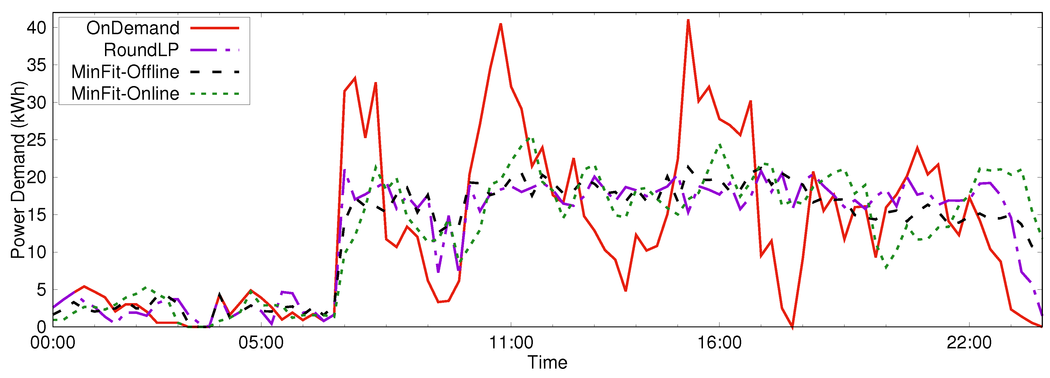
The second scenario we considered was the performance of the RoundLP, MinFit-Online, and MinFit-Offline algorithms with a large number of realistically generated jobs. Figure 4 shows the average power demand versus time of day for the OnDemand, RoundLP, MinFit-Online, and MinFit-Offline algorithms when scheduling 100 instances of 500 jobs over a 24 h period. The peak demands in k Wh were for OnDemand, for RoundLP, for MinFit-Offline, and for MinFit-Online.
5. Conclusions
In this work we presented the first approximation algorithm for the PDM problem for scheduling non-preemptible jobs, as well as an optimal dynamic programming algorithm that is fixed-parameter tractable and a heuristic approach that can be adapted to the online version of the problem. The problem occurs naturally in scheduling household power consuming jobs in a smart grid power system. Simulation results indicate that there is substantial opportunity to reduce the peak demand through deferred scheduling vs. on-demand. Avenues for future work include considering renewable energy when scheduling jobs. Integrating with renewable energy sources is becoming increasingly important for microgrids, and provides an additional mechanism for controlling peak demand and reducing dependency on non-renewable energy. Of critical importance, the available renewable energy curve may not be known with certainty, and so forecasts must be used. This introduces a random aspect to the performance of any schedule and so one might seek the schedule with the lowest expected non-renewable peak demand, etc. A second consideration is the trade-off between minimizing non-renewable peak demand and maximizing renewable energy consumption. Solutions of interest would be on the Pareto front of minimizing peak non-renewable demand and maximizing renewable energy use. Finally, the online version of PDM for non-preemptible jobs has not been explored in great depth.
Acknowledgments
This work was supported in part by National Science Foundation grant CNS-1156475.
Author Contributions
S.Y. and B.M. jointly conceived and designed the algorithms; S.Y. performed the experiments.
Conflicts of Interest
The authors declare no conflict of interest.
References
- Koutsopoulos, I.; Tassiulas, L. Optimal control policies for power demand scheduling in the smart grid. IEEE J. Sel. Areas Commun. 2012, 30, 1049–1060. [Google Scholar] [CrossRef]
- Fathi, M.; Bevrani, H. Adaptive Energy Consumption Scheduling for Connected Microgrids Under Demand Uncertainty. IEEE Trans. Power Deliv. 2013, 28, 1576–1583. [Google Scholar] [CrossRef]
- Yaw, S.; Mumey, B. An Exact Algorithm for Non-preemptive Peak Demand Job Scheduling. In Combinatorial Optimization and Applications; Lecture Notes in Computer Science; Springer: Cham, Switzerland, 2014; Volume 8881, pp. 3–12. [Google Scholar]
- Logenthiran, T.; Srinivasan, D.; Shun, T.Z. Demand Side Management in Smart Grid Using Heuristic Optimization. IEEE Trans. Smart Grid 2012, 3, 1244–1252. [Google Scholar] [CrossRef]
- Huang, Q.; Li, X.; Zhao, J.; Wu, D.; Li, X.Y. Social Networking Reduces Peak Power Consumption in Smart Grid. IEEE Trans. Smart Grid 2015, 6, 1403–1413. [Google Scholar] [CrossRef]
- Tang, S.; Huang, Q.; Li, X.Y.; Wu, D. Smoothing the energy consumption: Peak demand reduction in smart grid. In Proceedings of the 2013 IEEE INFOCOM, Turin, Italy, 14–19 April 2013; pp. 1133–1141. [Google Scholar]
- Yaw, S.; Mumey, B.; Mcdonald, E.; Lemke, J. Peak demand scheduling in the Smart Grid. In Proceedings of the 2014 IEEE International Conference on Smart Grid Communications (SmartGridComm), Venice, Italy, 3–6 November 2014; pp. 770–775. [Google Scholar]
- Roh, H.T.; Lee, J.W. Residential demand response scheduling with multiclass appliances in the smart grid. IEEE Trans. Smart Grid 2016, 7, 94–104. [Google Scholar] [CrossRef]
- Chuzhoy, J.; Guha, S.; Khanna, S.; Naor, J. Machine minimization for scheduling jobs with interval constraints. In Proceedings of the 45th Annual IEEE Symposium on Foundations of Computer Science, Rome, Italy, 17–19 October 2004; pp. 81–90. [Google Scholar]
- Cieliebak, M.; Erlebach, T.; Hennecke, F.; Weber, B.; Widmayer, P. Scheduling with release times and deadlines on a minimum number of machines. In Exploring New Frontiers of Theoretical Informatics; IFIP International Federation for Information Processing; Levy, J.J., Mayr, E., Mitchell, J., Eds.; Springer: New York, NY, USA, 2004; Volume 155, pp. 209–222. [Google Scholar]
- Ortmann, F.G.; Ntene, N.; van Vuuren, J.H. New and improved level heuristics for the rectangular strip packing and variable-sized bin packing problems. Eur. J. Oper. Res. 2010, 203, 306–315. [Google Scholar] [CrossRef]
- Gu, X.; Chen, G.; Xu, Y. Average-Case Performance Analysis of a 2D Strip Packing Algorithm—NFDH. J. Comb. Optim. 2005, 9, 19–34. [Google Scholar] [CrossRef]
- Baker, B.S.; Schwarz, J.S. Shelf algorithms for two-dimensional packing problems. SIAM J. Comput. 1983, 12, 508–525. [Google Scholar] [CrossRef]
- Raghavan, P.; Tompson, C.D. Randomized Rounding: A Technique for Provably Good Algorithms and Algorithmic Proofs. Combinatorica 1987, 7, 365–374. [Google Scholar] [CrossRef]
- Raghavan, P. Probabilistic construction of deterministic algorithms: Approximating packing integer programs. In Proceedings of the 27th Annual Symposium on Foundations of Computer Science, Toronto, ON, Canada, 27–29 October 1986; pp. 10–18. [Google Scholar]
- Kolter, J.Z.; Johnson, M.J. Redd: A public data set for energy disaggregation research. In Proceedings of the SustKDD Workshop on Data Mining Applications in Sustainability, San Diego, CA, USA, 21 August 2011. [Google Scholar]
Figure 1.
Sample jobs with arrival times, deadlines, lengths, and job configuration lists: , , , .

Figure 2.
Configuration trees for the jobs from Figure 1, with and pointers shown; pointers from leaves to themselves are omitted. An optimal solution is found by starting at the root of and following b and c pointers to a leaf of .
Figure 2.
Configuration trees for the jobs from Figure 1, with and pointers shown; pointers from leaves to themselves are omitted. An optimal solution is found by starting at the root of and following b and c pointers to a leaf of .

Figure 3.
Performance of peak demand minimization (PDM) scheduling algorithms in a smaller scenario where the optimal solution can be computed.
Figure 3.
Performance of peak demand minimization (PDM) scheduling algorithms in a smaller scenario where the optimal solution can be computed.
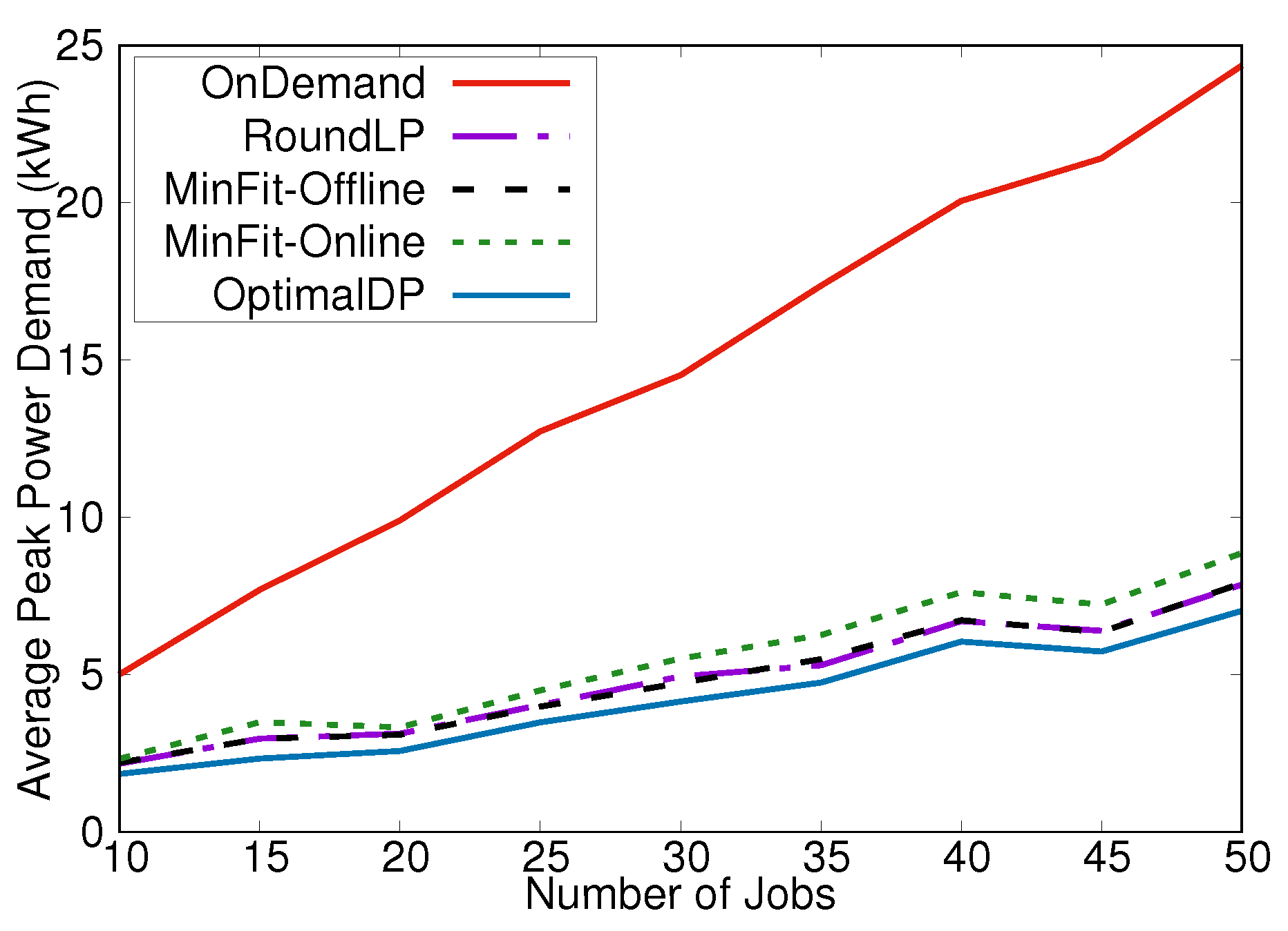
Figure 4.
Performance of PDM scheduling algorithms in a larger scenario. Total demand over time is plotted for each algorithm.
Figure 4.
Performance of PDM scheduling algorithms in a larger scenario. Total demand over time is plotted for each algorithm.

© 2017 by the authors. Licensee MDPI, Basel, Switzerland. This article is an open access article distributed under the terms and conditions of the Creative Commons Attribution (CC BY) license (http://creativecommons.org/licenses/by/4.0/).
Share and Cite
MDPI and ACS Style
Yaw, S.; Mumey, B. Scheduling Non-Preemptible Jobs to Minimize Peak Demand. Algorithms 2017, 10, 122. https://doi.org/10.3390/a10040122
AMA Style
Yaw S, Mumey B. Scheduling Non-Preemptible Jobs to Minimize Peak Demand. Algorithms. 2017; 10(4):122. https://doi.org/10.3390/a10040122
Chicago/Turabian StyleYaw, Sean, and Brendan Mumey. 2017. "Scheduling Non-Preemptible Jobs to Minimize Peak Demand" Algorithms 10, no. 4: 122. https://doi.org/10.3390/a10040122
Note that from the first issue of 2016, this journal uses article numbers instead of page numbers. See further details here.