An Indoor Collaborative Coefficient-Triangle APIT Localization Algorithm

1
CICAEET, School of Electronic & Information Enginnering, Nanjing University of Information Science & Technology, Nanjing 210044, China
2
Jiangsu Key Laboratory of Meteorological Observation and Information Processing, Nanjing University of Information Science & Technology, Nanjing 210044, China
3
Department of Telecommunications Engineering, Nanjing Institute of Technology, Nanjing 211167, China
*
Author to whom correspondence should be addressed.
Algorithms 2017, 10(4), 131; https://doi.org/10.3390/a10040131
Submission received: 23 September 2017
/
Revised: 20 November 2017
/
Accepted: 22 November 2017
/
Published: 28 November 2017
Abstract
:The Approximate Point-In-Triangulation (APIT) localization algorithm is a widely used indoor positioning technology due to its simplicity and low power consumption. However, in practice, In-to-Out misjudgments exist regularly in APIT, and a considerable amount of nodes cannot be positioned due to the low node density. To tackle this issue, a Collaborative Coefficient-triangle APIT Localization (CCAL) algorithm is proposed. Firstly, an effective triangle criterion is put forward to reduce the probability of In-to-Out misjudgment and reduce the computational complexity. Then, a further Received Signal Strength Indicator (RSSI) location and weighted triangle coordinate calculation method is adopted to reduce the positioning error. Meanwhile, the idea of iterative collaborative positioning of the positioned unknown nodes is introduced to remarkably expand the localization coverage rate. Simulation results show that the proposed algorithm outperforms APIT, RSSI, and other improved algorithms in terms of both node location error and localization coverage rate.
1. Introduction
Wireless sensor networks (WSNs) have been widely used in environment monitoring, military services and urban intelligent transportation [1]. The premise of WSNs is to obtain the node location information, partly because problems such as “where things happen” and “how to detect the geographic location of nodes” can only be solved with available location information. In addition, node positioning in the network helps to improve the performance through network power control, route selection, etc. [2].
Typically, the node location algorithms in a WSN can be classified into two categories: range-based and range-free schemes. The principle of range-based location algorithms is based on obtaining the relative location by measurement of the actual distance or angle among nodes. The classic range-based location algorithms include Angle of Arrival (AOA) algorithm [3], Time of Arrival (TOA) algorithm [4], the Time Difference on Arrival (TDOA) algorithm [5], and the Received Signal Strength Indicator (RSSI) algorithm [6]. Such algorithms have relatively high localization precision, but require high-performance hardware. The range-free location algorithms, on the other hand, can meet the localization precision in most applications without any additional hardware, such as a synchronous clock, which makes these algorithms suitable for complex communication conditions. Typical localization algorithms are the centroid algorithm [7], the Approximate Point-In-Triangulation APIT algorithm [8], the DV-Hop algorithm [9], the LACM algorithm [10], the LACMV algorithm [11], and the HPSO and BBO algorithm [12].
Among the above classical range-free location algorithms, the APIT localization scheme is widely used for localization estimation in wireless sensor networks, due to its simplicity and low power consumption. Furthermore, a number of efforts have been made to improve APIT algorithms.
In order to improve the robustness and the average positioning error, a virtual nodes-based APIT localization scheme is proposed [13]. To the effect of random deployment of all nodes, an improved centroid localization algorithm (ICLA) based on APIT is proposed [14]. Duo to produce more accurate location approach in isolation, a unified approach to localization is proposed [15]. To reduce costs per node, localization schemes based on event are proposed [16]. So as to reduce energy consumption and cost each node, the free-range location base schemes is proposed [17]. In order to increase the success ratio of localization, an approach to improve the position estimation accuracy of nodes using the Imperialist Competitive Algorithm is proposed [18]. So as to improve the poor locating performance of the DV-Hop algorithm, a localization algorithm based on SFLA and PSO is proposed [19]. In order to alleviate the so-called “flip ambiguity phenomenon,” a novel meta-heuristic localization technique for wireless sensor networks based on the harmony search algorithm is proposed [20].
However, it is important to note that the accuracy provided by the APIT algorithm depends on the position of the neighboring nodes, so it is easy to be subject to the effect of the density and distribution of sensor nodes.
In this paper, a Collaborative Coefficient-triangle APIT Localization (CCAL) algorithm is proposed, which introduces collaborative positioning to decrease the node positioning error and increase the localization coverage rate. MATLAB simulation results show that the CCAL algorithm outperforms the APIT, RSSI, and other improved algorithms in terms of both location error performance and coverage rate with low time complexity.
2. APIT Algorithm
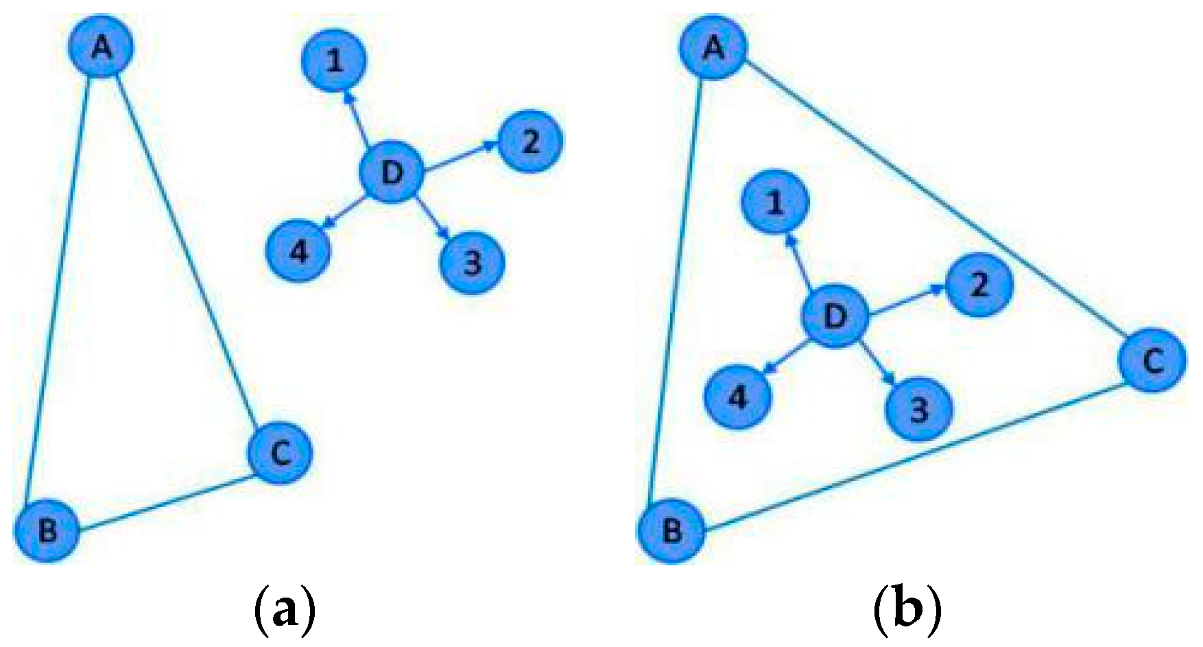
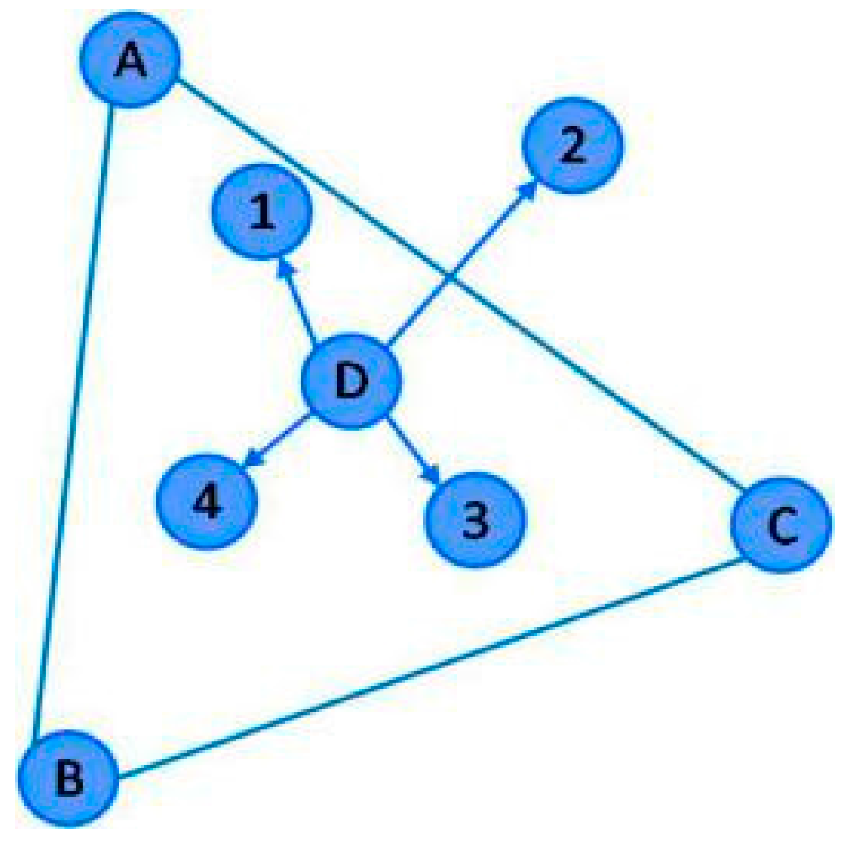
The principle of APIT is to judge whether the unknown node is inside the triangle using the surrounding nodes. As shown in Figure 1, the nodes surrounding an unknown node D are nodes 1, 2, 3 and 4. If there is a neighbor node that is simultaneously far away from or close to the anchor nodes A, B, C, it is considered that the unknown node is outside the triangle composed of A, B and C. Conversely, it is also considered to be inside triangle ABC.
In the APIT algorithm, the unknown node cannot be positioned when the number of surrounding anchor nodes is less than 3 or a valid triangle cannot be formed.
Meanwhile, the APIT positioning method calculates the coordinates of unknown nodes as the geometric center of the intersection, which is complicated and suboptimal [21]. Assume that there are N neighboring anchor nodes around the unknown node, and M valid triangles through the APIT judgment on triangles. The computation of the intersection of M valid triangles is time consuming [22]. Moreover, different valid triangles should have different roles in the evaluation which is not included in the traditional APIT.
Another significant problem of APIT is the In-to-Out misjudgment [23]. As shown in Figure 2, when the unknown node D is inside triangle ABC, and if node D refers to node 2, node D will be judged to be outside triangle ABC—this is In-to-Out misjudgment.
From the above discussion, the limitation of the APIT algorithm is the requirement of a high density of anchor nodes and a large communication radius of per anchor node. It is not suitable for a small to medium localization area. If it is the case that the above requirement cannot be met, a considerable number of nodes cannot be positioned and the probability of positioning error will be high. Moreover, with an increasing number of neighboring nodes, the positioning accuracy may decrease.
3. Collaborative Coefficient-Triangle APIT Localization Algorithm
Based on the limitation of APIT, a CCAL algorithm is proposed below, which involves an effective triangle criterion, an RSSI location and weighted triangle coordinate calculation method, and collaborative communication among nodes.
Firstly, to reduce the probability of In-to-Out misjudgment and computational complexity, an effective triangle criterion is introduced to permute and combine N anchor nodes to form triangles. Then, the APIT algorithm is used to determine whether the unknown node is inside a triangle, and if inside, the triangle can be judged to be a valid triangle. Meanwhile, the unknown node is determined to be outside a triangle only if the number of neighboring anchor nodes outside that triangle exceeds a certain threshold. The definition of threshold is shown below:
where is the scale factor, is the number of neighboring nodes involved in the judgment, and is the threshold for the number of qualified neighboring nodes. An effective triangle criterion may improve valid triangles on a limited number of directions in APIT. Hence, In-to-Out misjudgment can be greatly reduced.
To reduce the location error in APIT, a further RSSI-assisted location and weighted triangle coordinate calculation method is used. Using RSSI-assisted location, the distances between anchor nodes and unknown nodes of valid triangles are obtained. Then, the coordinates of the unknown nodes are estimated according to the maximum likelihood method.
In addition, the idea of iterative collaborative positioning is introduced to solve the positioning problem of unknown nodes. Specifically, the node flag of the positioned unknown nodes can be set to 2. The positioned nodes can be converted to special anchor nodes, and can broadcast their own location information to surrounding nodes. This can effectively compensate for the low anchor node density and poor anchor node distribution. The collaborative positioning scheme is detailed in the following.
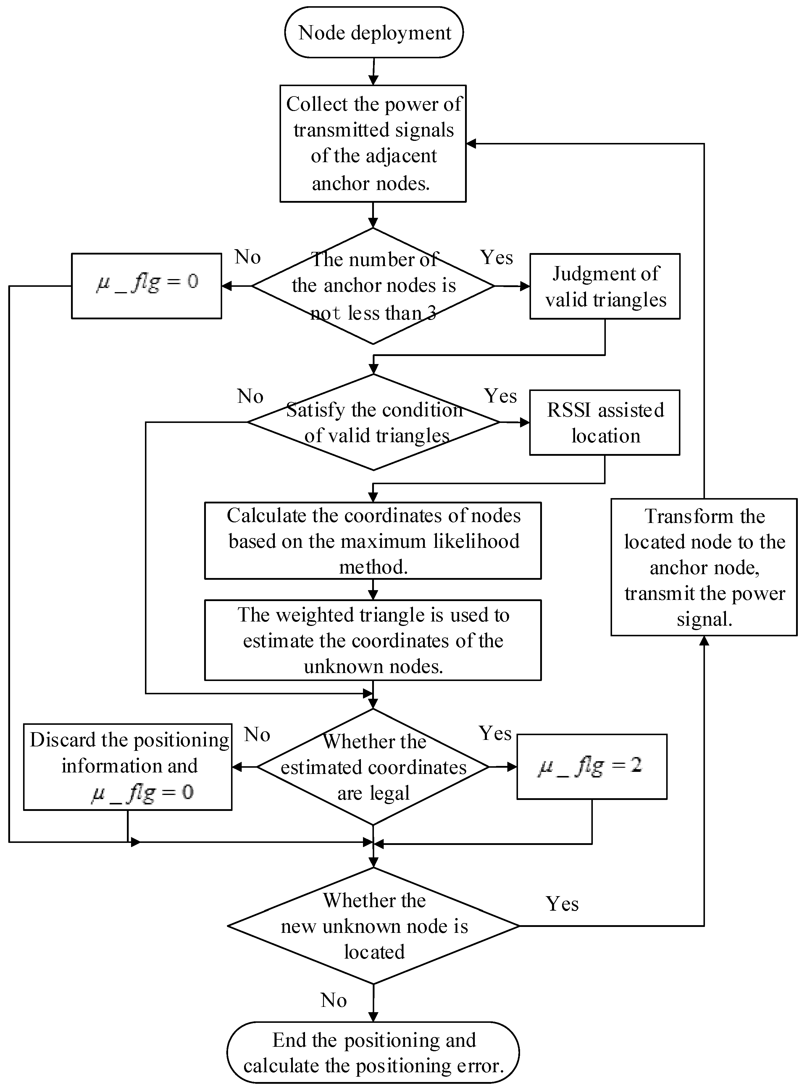
Based on the above discussion, Figure 3 shows the flow chart of the CCAL algorithm, and detailed steps are given below:
Step 1. Arrangement and definition of the nodes. The identification information of nodes is defined as follows: represents the unlocated unknown nodes, represents the known anchor nodes, and represents the located unknown nodes.
Step 2. For the unknown nodes, collect the power of transmitted signals from the adjacent anchor nodes.
Step 3. Judge whether the number of anchor nodes is not less than 3. If yes, proceed to Step 4; if no, the positioning cannot continue; set the identification of node .
Step 4. Judgment of valid triangles.
Permute and combine anchor nodes to form triangles. The APIT algorithm is used to determine whether the unknown node is inside a triangle, and if inside, the triangle can be judged to be a valid triangle. Meanwhile, the unknown node is determined as being outside one triangle only if the number of neighboring anchor nodes outside this triangle exceeds the threshold as in Equation (1).
Step 5. RSSI-assisted location.
Assume that there are M valid triangles acquired in Step 4. For valid triangle i, named , compute the distance from anchor nodes to unknown node , namely , , , as shown in Figure 4.
According to WiFi location technology, we can attain the transmitted power of anchor nodes and the signal strength , and then we can calculate the distance according to RSSI, as shown in Equation (2).
where represents the signal strength received by a node, represents the send energy, represents the signal strength received when the reference distance is , represents the scale factor between the path length and the path loss, represents a Gaussian random variable with a mean of 0 and a variance of .
Step 6. Calculate the coordinates of nodes based on the maximum likelihood method.
Assume that the coordinates of anchor nodes are , and the coordinates of the unknown node are . According to the relation between the distance and coordinates, the coordinates of the unknown node can be listed as follows:
Equation (3) can be transformed to a linear equation set, as shown in Equation (4):
Transform Equation (4) into the matrix form of the least squares method, as shown in Equation (5):
Here,
Thus, the coordinates of the unknown location can be derived as follows:
Step 7. Use the positioning method of the weighted triangle to estimate the coordinates of the unknown nodes.
Calculate the mean and standard variation of the distances , , for each valid triangle, and get , , where is the distance from the unknown node to anchor node i. Compute mean weighting factor and standard variation weighting factor .
Calculate two value pairs , of the unknown node coordinates as the mean-weighted and variation-weighted coordinates of M valid triangles, as shown in Equations (10) and (11). Then, estimate the coordinates of the unknown node as a combination of , , as shown in Equation (12), where and are the weighting coefficients of the mean and standard deviation respectively.
Step 8. Legality testing.
Assume that node A is the located node and D is the un-located node. Calculate the distance d from node A to node D. If the distance is within 120% of the communication radius of the unknown node, the estimated coordinates are legal, and the coordinate values are recorded and set the identification of the node to ; otherwise, the positioning error is considered to be too large, and the positioning result is invalid, discard the positioning information and set the identification of node .
Step 9. After each iteration of the localization algorithm, judge whether the new unknown node is located or not. If yes, transform the located node () into the anchor node, transmit the power signal to the neighboring area, and broadcast its positioning coordinates, then proceed to Step 2 and participate in the next round of location calculation; if not, end the positioning and calculate the positioning error.
4. Simulation and Analysis of Results
To verify the performance of the proposed algorithm, this paper uses parking lots as an example, and shows the simulation results by MATLAB. The default parameters of the WSN simulation in MATLAB are listed in Table 1, where we have considered the degree of irregularity (DOI) [24] of the waveform propagation for the simulation environment.
According to the experimental parameters in Table 1, the mean and standard deviation weighting factors, the node positioning error, the node localization coverage rate and time complexity are optimized. The node positioning error rate and the localization coverage rate are defined as follows:
In Equation (13), represents the positioning error of one single node, is the number of unknown nodes in the network, is the actual coordinate of the unknown nodes, is the located estimated coordinate, and is the communication radius of the unknown node.
The node localization coverage rate represents the ratio of the unknown nodes that can be located for all the unknown nodes in the network. Assume that there are unknown nodes in the network, h nodes can be located, and then the node localization coverage rate can be indicated as:
4.1. Optimization of the Mean and Standard Deviation Weighting Factors
According to Equation (1), is set to 0.2, and according to Equation (12), the impact of the mean and standard deviation weighting factors is given by = 0.25, 0.5, 0.75; = 0.25, 0.5, 0.75 respectively.
Thus, results are shown in Figure 5, where the x-coordinate is the proportion of the anchor nodes, and the y-coordinate is the node positioning error. Here, the proportion of anchor nodes was generally between 20% and 30% in the actual network deployment.
From Figure 5, it can be seen that the node positioning error decreased as the proportion of anchor nodes increased. The minimum positioning error was obtained when the weighting factors were , . Therefore, these weighting factors were adopted in the following simulations.
4.2. Node Localization Coverage Rate of the Proposed Localization Algorithm
The node localization coverage rate is another important indicator used to assess the performance of a positioning system.
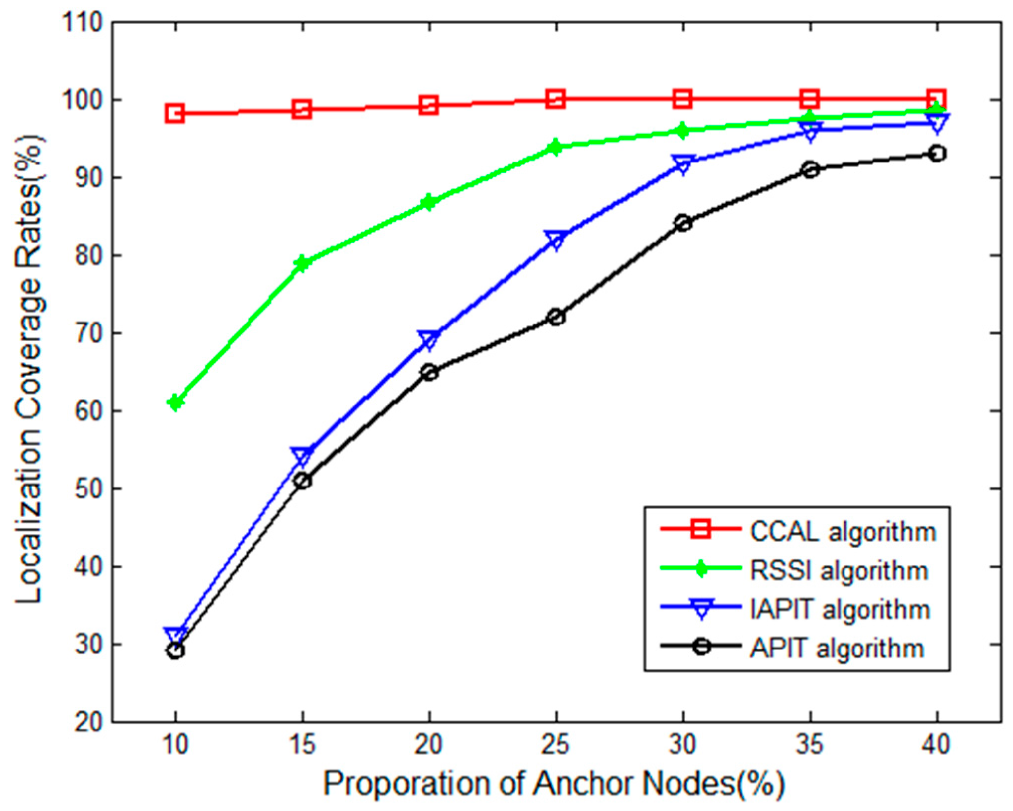
Figure 6 shows the curves of node localization coverage rates with the increase in the proportion of anchor nodes in the CCAL, RSSI, IAPIT and APIT algorithms.
As shown in Figure 6, when the proportion of anchor nodes increased, the node localization coverage rates of the four localization algorithms increased. When the proportion of anchor nodes was certain, the node localization coverage rate of CCAL was the highest, basically remaining at 100%. This is because the CCAL algorithm turns the positioned unknown nodes into anchor nodes, and uses the maximum likelihood method and legality testing, thereby greatly reducing the number of nodes that cannot be positioned when the proportion of anchor nodes is small.
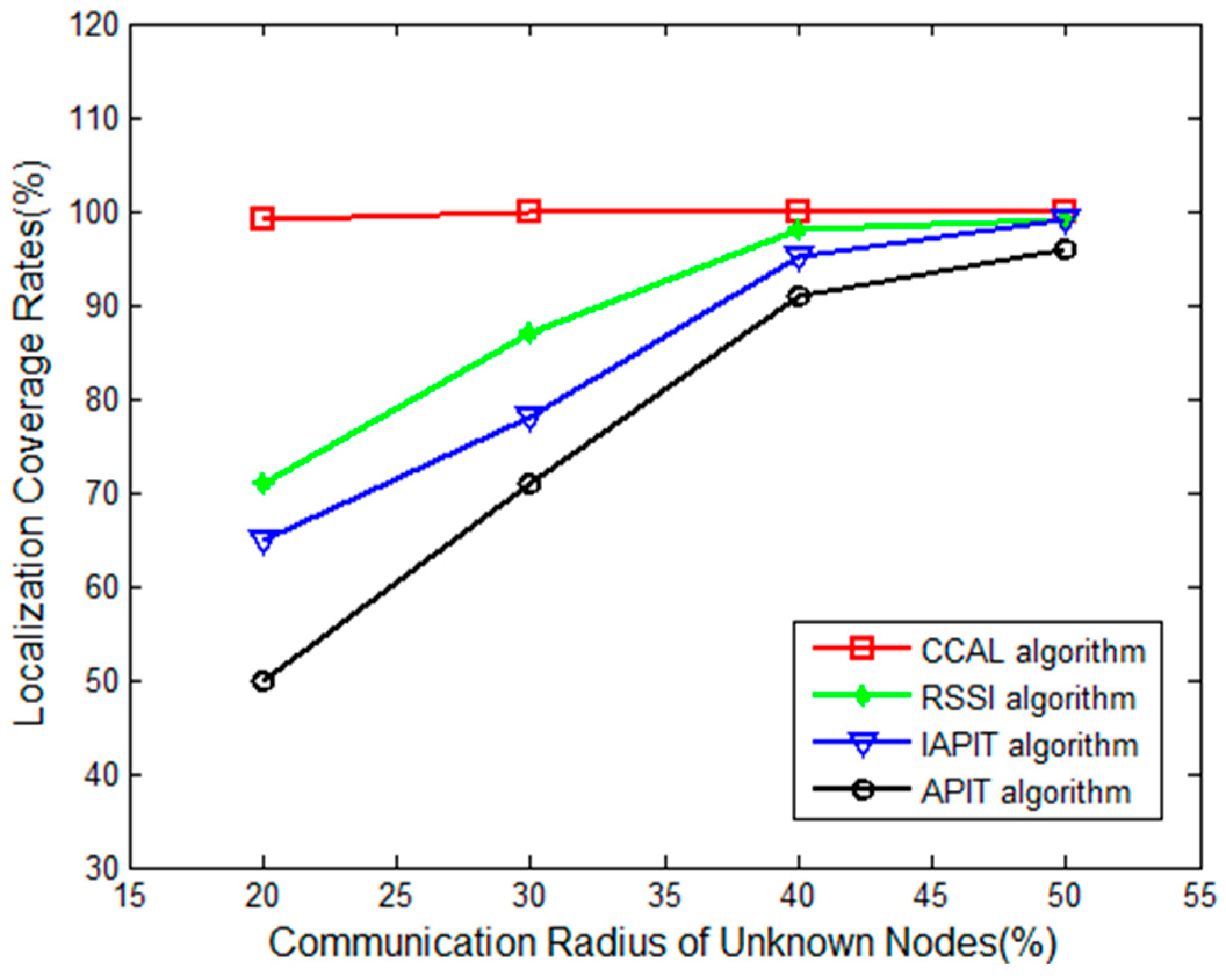
Figure 7 shows the curves of node localization coverage rates with the increase in the communication radius of the unknown node, while the proportion of anchor nodes remains 20%.
As shown in Figure 7, the node localization coverage rate of RSSI, APIT and IAPIT clearly increased when the communication radius of the unknown node increased. This is because there are less than three anchor nodes surrounding many unknown nodes when the communication radius is smaller. On the one hand, many nodes cannot be positioned in these three algorithms. On the other hand, the localization coverage rates of the CCAL algorithm change slowly. This is due to the fact that the CCAL algorithm uses the maximum likelihood method to estimate the coordinates of nodes that cannot be positioned, thereby ensuring the node localization coverage rate.
4.3. Positioning Error of the Proposed Localization Algorithm
In a WSN positioning system, the proportion of anchor nodes has a great influence on the performance of the localization algorithm. The experiments in [25] were conducted as follows:
In the experiments, assume that the weighting coefficients of the mean value and the standard deviation are and . The positioning errors of the CCAL algorithm, RSSI algorithm, IAPIT algorithm [26] and APIT algorithm were determined by varying the ratio of the anchor nodes and the communication radius of the unknown nodes.
Simulations of the CCAL algorithm, RSSI algorithm, IAPIT algorithm, and APIT algorithm were carried out when the communication radius of unknown nodes remained 30 m and the proportion of anchor nodes varied in a wider range. Figure 8 shows the resulting curves of the node positioning errors of the localization algorithms with the increase in the proportion of anchor nodes.
It is shown in Figure 8 that the CCAL algorithm had the best performance. Generally, the positioning error of CCAL is 15% smaller than that of APIT, 13% smaller than that of the RSSI algorithm, and 8% smaller than that of the IAPIT algorithm. This is because the CCAL algorithm introduces legality testing to the estimated unknown nodes, which avoids the effect of those nodes with large positioning error.
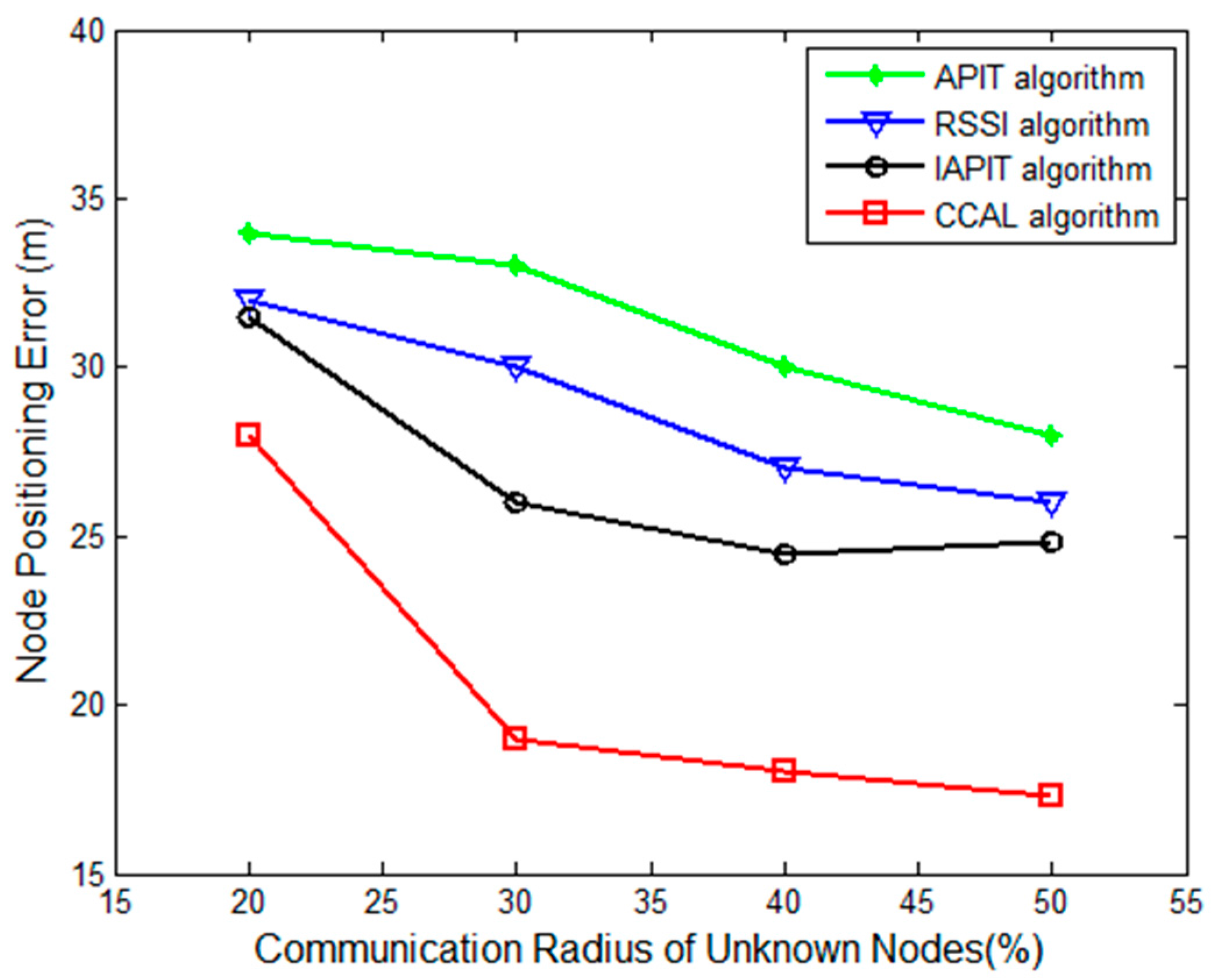
Simulation was also carried out when the proportion of anchor nodes remained 20% and the communication radius of unknown nodes varied. The results are shown in Figure 9.
As shown in Figure 9, the positioning errors of four algorithms were reduced when the communication radius of unknown nodes increased, and the positioning error of the CCAL algorithm was the smallest, i.e., 5% smaller than that of IAPIT, 10% smaller than that of RSSI, and 14% smaller than that of APIT. This is because when the communication radius of unknown nodes increases, the number of neighboring anchor nodes and valid triangles increases, and the positioning error decreases.
4.4. Time Complexity of the Proposed Localization Algorithm
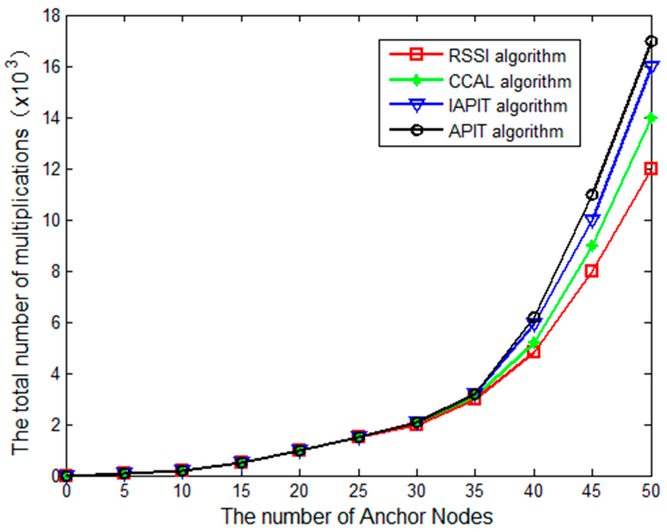
The time complexity in [27] was used to analyze the performance of each algorithm, and Figure 10 shows the results of four localization algorithms with different numbers of anchor nodes.
As shown in Figure 10, the time complexity of the CCAL algorithm increased by 12% compared to the RSSI algorithm, but was reduced by 20% compared to the APIT algorithm, and 11% compared to the IAPIT algorithm. The CCAL algorithm needs to judge whether the unknown node is outside the triangle, which increases the time complexity.
5. Conclusions
A CCAL (Coefficient-triangle APIT Localization) algorithm has been proposed for indoor collaborative localization, which remarkably expands the localization coverage rate by introducing the idea of iterative collaborative positioning. Furthermore, the probability of In-to-Out misjudgment and positioning error is greatly reduced by introducing an effective triangle criterion, as well as a RSSI-based weighted triangle coordinate calculation method. Simulations in MATLAB have verified the performance improvement of the CCAL algorithm and the simulation results reveal an improvement of about 8% in positioning accuracy compared to the IAPIT algorithm, 12% improvement compared to the RSSI algorithm and 15% improvement compared to the APIT algorithm; the localization coverage rate is increased by 15% relative to RSSI, 20% relative to IAPIT, and 30% relative to APIT.
Acknowledgments
This research was supported by National Natural Science Foundation of China (61705109), Natural Science Foundation of the Jiangsu Higher Education Institutions of China (Grant No. 12KJA510001) and was funded by the Priority Academic Program Development of Jiangsu Higher Education Institution, China.
Author Contributions
Su-Ting Chen and Peng Li conceived and designed the experiments; Peng Li performed the experiments; Chuang Zhang and Yan-Yan Zhang analyzed the data; Liang-Bao Jiao contributed reagents/materials/analysis tools; Su-Ting Chen wrote the paper.
Conflicts of Interest
The authors declare no conflict of interest.
References
- Alippi, C.; Camplani, R.; Galperti, C.; Roveri, M. A Robust, Adaptive, Solar-Powered WSN Framework for Aquatic Environmental Monitoring. IEEE Sens. J. 2011, 11, 45–55. [Google Scholar] [CrossRef]
- Chi, Q.; Yan, H.; Zhang, C.; Pang, Z.; Da Xu, L. A Reconfigurable Smart Sensor Interface for Industrial WSN in IoT Environment. IEEE Trans. Ind. Inform. 2014, 10, 1417–1425. [Google Scholar]
- Deng, P.; Fan, P.Z. An AOA assisted TOA positioning system. In Proceedings of the WCC-ICCT International Conference on Communication Technology Proceedings, Beijing, China, 21–25 August 2000; pp. 1501–1504. [Google Scholar]
- Patwari, N.; Ash, J.N.; Kyperountas, S.; Hero, A.O.; Moses, R.L.; Correal, N.S. Locating the nodes: Cooperative localization in wireless sensor networks. IEEE Signal Process. Mag. 2005, 22, 54–69. [Google Scholar] [CrossRef]
- Priyantha, N.B.; Chakraborty, A.; Balakrishnan, H. The Cricket location-support system. In Proceedings of the 6th Annual International Conference on Mobile Computing and Networking, Boston, MA, USA, 6–11 August 2000; pp. 32–43. [Google Scholar]
- Srinivasan, K.; Levis, P. RSSI is under appreciated. In Proceedings of the Third Workshop on Embedded Networked Sensors (EmNets); Stanford Information Networks Group: Stanford, CA, USA, 2006. [Google Scholar]
- Bulusu, N.; Heidemann, J.; Estrin, D. GPS-less low-cost outdoor localization for very small devices. IEEE Pers. Commun. 2000, 7, 28–34. [Google Scholar] [CrossRef]
- He, T.; Huang, C.; Blum, B.M.; Stankovic, J.A.; Abdelzaher, T. Range-free localization schemes for large scale sensor networks. In Proceedings of the 9th Annual International Conference on Mobile Computing and Networking, San Diego, CA, USA, 14–19 September 2003; pp. 81–95. [Google Scholar]
- Liu, C.; Liu, S.; Zhang, W.; Zhao, D. The Performance Evaluation of Hybrid Localization Algorithm in Wireless Sensor Networks. Mob. Netw. Appl. 2016, 21, 994–1001. [Google Scholar] [CrossRef]
- Cabero, J.M.; Olabarrieta, I.; Gil-López, S.; Del Ser, J.; Martín, J.L. Range-free localization algorithm based on connectivity and motion. Wirel. Netw. 2014, 20, 2287–2305. [Google Scholar] [CrossRef]
- Cabero, J.M.; Olabarrieta, I.I.; Gil-López, S.; Del Ser, J.; Martín, J.L. A novel range-free localization algorithm to turn connectivity traces and motion data into localization information. Ad Hoc Netw. 2014, 20, 36–52. [Google Scholar] [CrossRef]
- Kumar, A.; Khosla, A.; Saini, J.S.; Sidhu, S.S. Range-free 3D node localization in anisotropic wireless sensor networks. Appl. Soft Comput. 2015, 34, 438–448. [Google Scholar] [CrossRef]
- Feng, C.; Liu, Z. A New Node Self-Localization Algorithm Based RSSI for Wireless Sensor Networks. In Proceedings of the 2013 5th International Conference on Computational and Information Sciences, Shiyang, China, 21–23 June 2013; pp. 1616–1619. [Google Scholar]
- Li, L.; Wu, Y.; Ren, Y.; Yu, N. A RSSI Localization Algorithm based on Interval Analysis for Indoor Wireless Sensor Networks. In Proceedings of the 2013 IEEE International Conference on Green Computing and Communications and IEEE Internet of Things and IEEE Cyber, Physical and Social Computing, Beijing, China, 20–23 August 2013; pp. 434–437. [Google Scholar]
- Zhou, G.; He, T.; Krishnamurthy, S.; Stankovic, J.A. Impact pf Radio Irregularity on Wireless Sensor Networks. In Proceedings of the 2th International Conference on Mobile Systems Applications and Services, Boston, MA, USA, 6–9 June 2004; pp. 125–138. [Google Scholar]
- Wang, J.Z.; Jin, H. Improvement on APIT Localization Algorithms for Wireless Sensor Networks. In Proceedings of the International Conference on Networks Security, Wireless Communications and Trusted Computing, Wuhan, China, 25–26 April 2009; pp. 719–723. [Google Scholar]
- Quattrone, A.; Kulik, L.; Tanin, E. Combining Range-Based and Range-Free Methods: A Unified Approach for Localization. In Proceedings of the 23rd SIGSPATIAL International Conference on Advances in Geographic Information Systems, Seattle, WA, USA, 3–6 November 2015. [Google Scholar]
- Stoleru, R.; He, T.; Stankovic, J.A. Range-free localization. In Secure Localization and Time Synchronization for Wireless Sensor and Ad Hoc Networks; Springer: Boston, MA, USA, 2007; pp. 3–31. [Google Scholar]
- Khan, H.; Hayat, M.N.; Rehman, Z.U. Wireless sensor networks free-range base localization schemes: A comprehensive survey. In Proceedings of the IEEE International Conference on Communication, Computing and Digital Systems (C-CODE), Islamabad, Pakistan, 8–9 March 2017; pp. 144–147. [Google Scholar]
- Sayadnavard, M.H.; Haghighat, A.T.; Abdechiri, M. Wireless sensor network localization using imperialist competitive algorithm. In Proceedings of the 3rd IEEE International Conference on Computer Science and Information Technology (ICCSIT), Chengdu, China, 9–11 July 2010; Volume 9, pp. 818–822. [Google Scholar]
- Ren, W.; Zhao, C. A localization algorithm based On SFLA and PSO for wireless sensor network. Inf. Technol. J. 2013, 12, 502–505. [Google Scholar] [CrossRef]
- Manjarres, D.; Del Ser, J.; Gil-Lopez, S.; Vecchio, M.; Landa-Torres, I.; Lopez-Valcarce, R. A novel heuristic approach for distance-and connectivity-based multihop node localization in wireless sensor networks. Soft Comput. 2013, 17, 17–28. [Google Scholar] [CrossRef]
- Yong, Z.; Shixiong, X.; Shifei, D.; Lei, Z.; Xin, A. An Improved APIT Node Self-Localization Algorithm in WSN Based on Triangle-Center Scan. J. Comput. Res. Dev. 2009, 46, 566–574. [Google Scholar]
- Niculescu, D.; Nath, B. DV Based Positioning in Ad Hoc Networks. Telecommun. Syst. 2003, 22, 267–280. [Google Scholar] [CrossRef]
- Liu, J.; Wang, Z.; Yao, M.; Qiu, Z. VN-APIT: Virtual nodes-based range-free APIT localization scheme for WSN. Wirel. Netw. 2016, 22, 867–878. [Google Scholar] [CrossRef]
- Salim, F.; Williams, M.; Sony, N.; Pena, M.D.; Petrov, Y.; Saad, A.A.; Wu, B. Visualization of wireless sensor networks using ZigBee’s Received Signal Strength Indicator (RSSI) for indoor localization and tracking. In Proceedings of the 2014 IEEE International Conference on Pervasive Computing and Communication Workshops (PERCOM Workshops), Budapest, Hungary, 24–28 March 2014; pp. 575–580. [Google Scholar]
- Liu, Y.; Yi, X.; He, Y. A Novel Centroid Localization for Wireless Sensor Networks. Int. J. Distrib. Sens. Netw. 2012, 8. [Google Scholar] [CrossRef]
Figure 1.
Schematic diagram of Approximate Point-In-Triangulation (APIT). (a) Outside the triangle. (b) Inside the triangle.
Figure 1.
Schematic diagram of Approximate Point-In-Triangulation (APIT). (a) Outside the triangle. (b) Inside the triangle.

Figure 2.
In-to-Out Misjudgment of the APIT algorithm.

Figure 3.
Flow chart of Collaborative Coefficient-triangle APIT Localization (CCAL) algorithm.

Figure 4.
The principle of trilateration.
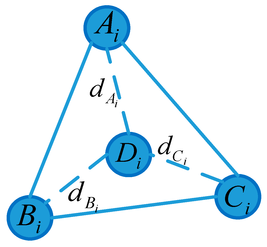
Figure 5.
Positioning error curves of variable weighting factors.
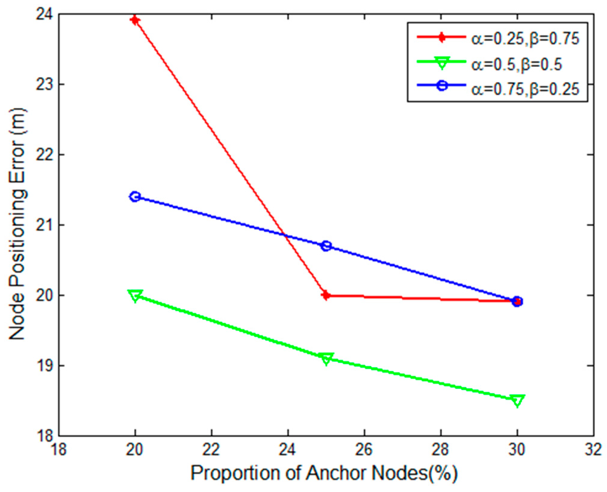
Figure 6.
Curves of localization coverage rates with the proportion of anchor nodes varying.

Figure 7.
Curves of the localization coverage rate with various communication radii of unknown nodes.
Figure 7.
Curves of the localization coverage rate with various communication radii of unknown nodes.

Figure 8.
Positioning error curves with the proportion of anchor nodes varying.
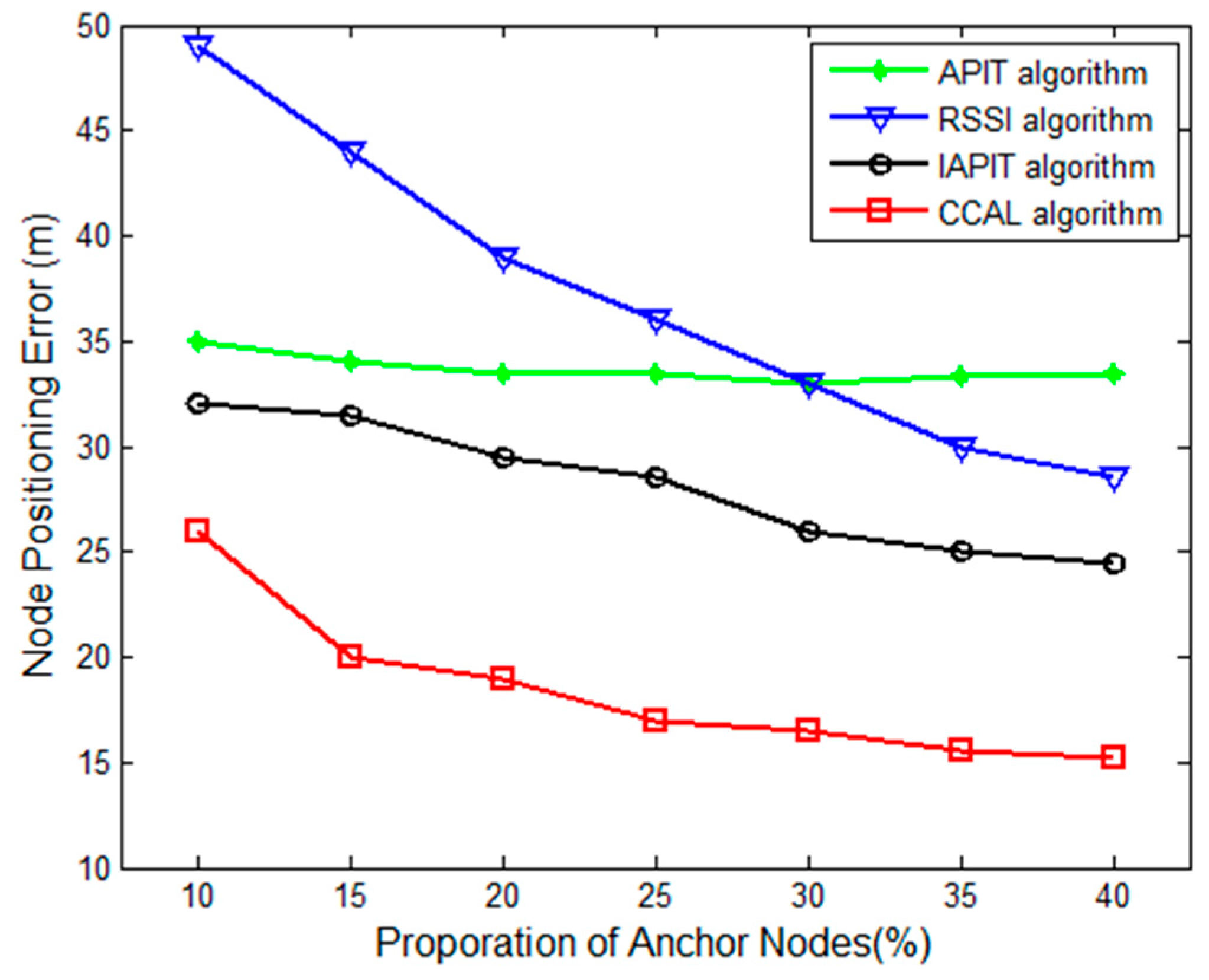
Figure 9.
Positioning error curves with the communication radius varying.

Figure 10.
The time complexity of different algorithms.


Table 1.
Default wireless sensor network (WSN) parameters in the algorithm simulation.
| Parameter | Configuration Information |
|---|---|
| Location area | 100 m × 100 m |
| Number of all nodes | 100 |
| Transmission model | DOI |
| Signaling irregularity | 0.005 |
| Send energy | 0 dBm |
| Reference distance | 1 m |
| Signal strength | 55 dBm |
| Scale factor | 4 |
© 2017 by the authors. Licensee MDPI, Basel, Switzerland. This article is an open access article distributed under the terms and conditions of the Creative Commons Attribution (CC BY) license (http://creativecommons.org/licenses/by/4.0/).
Share and Cite
MDPI and ACS Style
Chen, S.-T.; Zhang, C.; Li, P.; Zhang, Y.-Y.; Jiao, L.-B. An Indoor Collaborative Coefficient-Triangle APIT Localization Algorithm. Algorithms 2017, 10, 131. https://doi.org/10.3390/a10040131
AMA Style
Chen S-T, Zhang C, Li P, Zhang Y-Y, Jiao L-B. An Indoor Collaborative Coefficient-Triangle APIT Localization Algorithm. Algorithms. 2017; 10(4):131. https://doi.org/10.3390/a10040131
Chicago/Turabian StyleChen, Su-Ting, Chuang Zhang, Peng Li, Yan-Yan Zhang, and Liang-Bao Jiao. 2017. "An Indoor Collaborative Coefficient-Triangle APIT Localization Algorithm" Algorithms 10, no. 4: 131. https://doi.org/10.3390/a10040131
Note that from the first issue of 2016, this journal uses article numbers instead of page numbers. See further details here.