Algebraic Dynamic Programming on Trees


1
Bioinformatics Group, Department of Computer Science, Interdisciplinary Center for Bioinformatics, University Leipzig, Härtelstraße 16-18, D-04107 Leipzig, Germany
2
Max Planck Institute for Mathematics in the Sciences, Inselstraße 22, D-04103 Leipzig, Germany
3
German Centre for Integrative Biodiversity Research (iDiv) Halle-Jena-Leipzig, Competence Center for Scalable Data Services and Solutions, and Leipzig Research Center for Civilization Diseases, University Leipzig, D-04103 Leipzig, Germany
4
Fraunhofer Institute for Cell Therapy and Immunology, Perlickstrasse 1, D-04103 Leipzig, Germany
5
Institute for Theoretical Chemistry, University of Vienna, Währingerstraße 17, A-1090 Wien, Austria
6
Center for RNA in Technology and Health, Univ. Copenhagen, Grønnegårdsvej 3, 1870 Frederiksberg C, Denmark
7
Santa Fe Institute, 1399 Hyde Park Rd., Santa Fe, NM 87501, USA
*
Author to whom correspondence should be addressed.
Algorithms 2017, 10(4), 135; https://doi.org/10.3390/a10040135
Submission received: 13 October 2017
/
Revised: 1 December 2017
/
Accepted: 2 December 2017
/
Published: 6 December 2017
Abstract
:Where string grammars describe how to generate and parse strings, tree grammars describe how to generate and parse trees. We show how to extend generalized algebraic dynamic programming to tree grammars. The resulting dynamic programming algorithms are efficient and provide the complete feature set available to string grammars, including automatic generation of outside parsers and algebra products for efficient backtracking. The complete parsing infrastructure is available as an embedded domain-specific language in Haskell. In addition to the formal framework, we provide implementations for both tree alignment and tree editing. Both algorithms are in active use in, among others, the area of bioinformatics, where optimization problems on trees are of considerable practical importance. This framework and the accompanying algorithms provide a beneficial starting point for developing complex grammars with tree- and forest-based inputs.
1. Introduction
Dynamic programming (DP) is a general paradigm for solving combinatorial problems with a search space of exponential size in polynomial time (and space). The key idea is that the optimal solution for the overall problem can be constructed by combining the optimal solutions to subproblems (known as optimal substructure). During the recursive deconstruction of the original problem instance, the same smaller subproblems (known as overlapping subproblems) are required repeatedly and thus memoized. DP is typically applied to optimization and (weighted) enumeration problems. Not all such problems are amenable to this strategy however.
Bellman’s principle [1] codifies the key necessary condition, the intuition of which can be expressed for optimization problems as follows: The optimal solution of any (sub)problem can be obtained as a suitable combination of optimal solutions of its subproblems.
In Bioinformatics, DP algorithms are a useful tool to solve tasks such as sequence alignment [2] or RNA secondary structure prediction [3,4]. Here, the description of dynamic programming algorithms as formal grammars is common practice [5]. Problems whose natural input structure is a tree typically have no satisfactory solution using an encoding as strings, because one “dimension” within the input is lost. As a consequence, solutions to seemingly similar string problems can be very different. A simple example is comparison of two patterns of matching parentheses:
	  ((((((())))))) ((((((())))))--)
	  (((((()))))()) ((((((--)))))())
On the l.h.s., they are interpreted as strings differing by two substitutions. On the r.h.s., interpreted as trees the difference is the insertion and deletion of matching pairs in each pattern.
A simple, yet often encountered, example of a tree is the structure of a text such as a book. Books are divided into chapters, sections, subsections, and blocks of text, imposing a hierarchical structure in addition to the linear order of words. Many other formats for data exchange are based on similar structures, including json and xml. In bioinformatics, tree structures encode, among others, the (secondary) structure of RNA and phylogenetic trees, hence DP algorithms on trees have a long history in computational biology. Well-studied problems include the computation of parsimony and likelihood scores for given phylogenies [6], tree alignment [7] and tree editing [8], reconciliation of phylogenetic trees [9], and RNA secondary structure comparison [10,11]. Giegerich and Touzet [12] developed a system of inverse coupled rewrite systems (ICOREs) which unify dynamic programming on sequences and trees. Rules written in this system bear a certain semblance to our system. We are not aware of an implementation of ICORES, however, making comparisons beyond the formalism difficult. All of these approaches use trees and/or forests as input structures. Aims and methods, however, are different. We argue here that a common high-level framework will substantially simplify the design and development of such algorithms and thus provide a very useful addition to the toolbox of someone working with tree-like data. There are implementations for most of the problems mentioned above. However, they use problem-specific choices for the recursions and memoization tables that seem to be hard to generalize. A particularly difficult challenge is the construction of DP algorithms that are not only complete but also semantically unambiguous. The latter property ensures that each configuration is considered only once, so that the DP recursion correctly counts and thus can be used to compute partition functions. A recent example is the approach of [7] to tree alignment. In general, recognizing ambiguity for context-free grammars is undecidable [13,14]. There are, however, quite efficient heuristics that can be used successfully to prove that string grammars describing many problems in computational biology are unambiguous [15]. The aim of the present contribution is to develop a general framework as a generic basis for the design and implementations of DP algorithms on trees and forests. We focus here on well-known algorithms with existing implementations as examples because in these cases the advantages of the ADP approach can be discussed directly in comparison to the literature. Since DP algorithms are usually formulated in terms of recursion equations, their structure is usually reflected by formal grammars. These are more compact than the recursions and more easily lend themselves to direct comparisons. In this way, we therefore can compare results and make sure that the algorithms are either unambiguous or work well even in the ambiguous case. Here, ambiguity does not affect the running time of the algorithms.
The most difficult issue in this context is to identify a sufficiently generic representation of the search spaces on which the individual application problems are defined. Following [16], a natural starting point is a formal grammar G as a rewriting system specifying a set of rules on how to generate strings or read strings of the corresponding language . The benefit of using formal grammars compared to, say, explicit recurrences, is mostly in the high-level description of the solution space defined by the problem at hand. For formal grammars describing dynamic programming problems on strings several approaches have been developed in recent years [16,17,18,19,20]. Formal grammars can describe tree languages just as well as string languages. This opens up the benefits of using formal languages (in abstracting away the minutia of implementation details) for this expanded input type [21,22].
Our contributions are twofold. First, we provide a theoretical framework for describing formal languages on trees. We give a small set of combinators—functions that formalize the recursive deconstruction of a given tree structure into smaller components—for the design of such formal languages. Second, we show that an implementation in the ADPfusion [18] variant of algebraic dynamic programming (ADP) [23] yields short and elegant implementations for a number of well-known algorithms on tree structures.
2. Algebraic Dynamic Programming (ADP)
Algebraic dynamic programming (ADP) [18,25] is designed around the idea of higher order programming and starts from the realization that a dynamic programming algorithm can be separated into four parts: (i) grammar, (ii) algebra, (iii) signature, and (iv) memoization. These four components are devised and written separately and combined to form possible solutions. One advantage of ADP is that the decoupling of the individual components makes each individual component much easier to design and implement. Another advantage is that different components can be re-used easily. This is in particular true for the grammar, which defines the search space. Hence, it needs to be specified only once. The grammar only specifies the input alphabet and the production rules on how to split the input data structure in subparts. The algebra specifies the cost function and the selection criterion, also called objective function, and thus defines formally what is considered as an “optimal” solution. Based on the objective function, the optimal solution is selected from the possible solutions. The scope of the evaluation algebra is quite broad. It can be used e.g., to count and list prioritized (sub-)optimal solutions. The signature is used as a connecting element between grammar and algebra such that they can be re-used and exchanged independently from each other as long as they fit to the signature. In order to recursively use subsolutions to the problem, they are stored using a data structure easy to save and look-up the subsolution to the current instance. This is called memoization. In this section, the four parts of ADP will be explained using string alignment as an example.
Before we delve into dynamic programming on trees and forests, we recapitulate the notations for the case of dynamic programming on strings. The problem instance is the venerable Needleman-Wunsch [26] string alignment algorithm. The algorithm expects two strings as input. When run, it produces a score based on the number of matches, mismatches, deletions, and insertions that are needed to rewrite the first into the second input string.
One normally assigns a positive score to a match, and negative scores to mismatches, deletions, and insertions. With the separation of concerns provided by algebraic dynamic programming, the algebra that encodes this scoring becomes almost trivial, while the logic of the algorithm, or the encoding of the search space of all possible alignments in the form of a grammar, is the main problem. As such, we mostly concentrate on the grammars, delegating scoring algebras to a secondary place.
A simple version of the Needleman-Wunsch algorithm [26] is given by:
The grammar has one 2-line symbol on the left-hand side, the non-terminal . The notion of two lines of X is indicative of the algorithm requiring two input sequences. This notion will be made more formal in the next section. Here, X is a non-terminal of the grammar, a a terminal character, $ the termination symbol and ‘−’ the “no input read”-symbol. Non-terminals such as are always regarded as one symbol, and can be replaced by any of the rules on the right-hand side that have said symbol on the left-hand side. Terminals, say , act on individual inputs, here not moving on the first input, but reading a character “into” a on the second input. In theory of automata it is customary to refer to independent inputs as “input tapes”. The operations of the grammar can be explained for each symbol individually, while grouping into columns indicates that the symbol on each line, and thereby input, operates in lockstep with the other symbols in the column. Multiple tapes thus are not processed independently, i.e., ‘actions’ are taken concurrently on all tapes. Since we consider the insertion of a gap symbol also as an ‘action’, it is not allowed to insert gap symbols on all the tapes at the same time. Hence, in each step at least one of the tapes is ‘consuming’ an input character. The algorithm is therefore guaranteed to terminate.
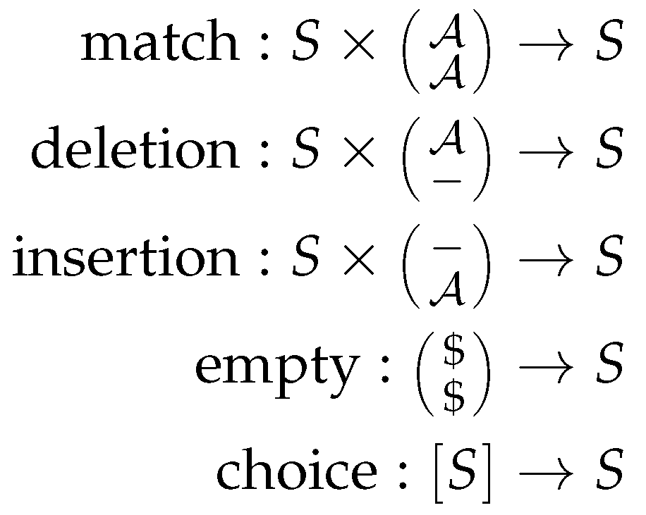
The grammar defines 4 different cases: (i) matching the current positions of the input strings, (ii)–(iii) inserting a gap symbol in one or the other of the input strings or the case (iv) when both input strings are empty. As the algorithm should return the best possible alignment of the input strings, each of the production rules is assigned a scoring function in the scoring algebra. The scoring function will take the current score and return an updated score including the weight for the current case (match, deletion or insertion). Figure 1 shows two different scoring algebras for the grammar of string alignment, with being the input alphabet, and S the set of scores. Thus, for each grammar, we can choose a scoring algebra independently. The choice function corresponds to the objective function of the dynamic programming algorithm. As it is used to rank given (sub)solutions, it is not part of the grammar but part of the scoring algebra and the signature, as seen in Figure 1 and Figure 2.
The signature in ADP provides a set of function symbols that provide the glue between the grammar and the algebra. Thus, we define the type signatures for each of the scoring functions, analogously to type signatures found in functional programming. Figure 2 shows the signature for the Needleman-Wunsch algorithm. This signature fits to both scoring algebras and the grammar. Here, is the input alphabet, and S the set of scores as above.
The last part needed for ADP is the memoization to store the subsolutions. For the Needleman-Wunsch algorithm we simply use a matrix of size where s and t are the lengths of the input strings to store the subsolutions.
3. DP Algorithms on Trees and Forests
Algebraic dynamic programming [25] in its original form was designed for single-sequence problems. Alignment-style problems were solved by concatenating the two inputs and including a separator.
Originally, ADPfusion [18] was designed along the lines of ADP, but gained provisions to abstract over both the input type(s), and the index space with the advent of generalized algebraic dynamic programming [17,24,27,28,29] inputs were generalized to strings and sets, as well as multiple tapes (or inputs) of those.
Trees as data structures sit “somehow between” strings and sets. They have more complex structures, in that each node not only has siblings, but also children compared to lists which only have siblings for each node in the list or string. Sets on the other hand are typically used based on the principle of having edges between all nodes, with each edge having a particular weight. This alone makes trees an interesting structure to design a formal dynamic programming environment for. Tree and forest structures have, as discussed above, important functions in (for example) bioinformatics and linguistics.
DP algorithms can be applied not only to just one input structure but also to two or more independent inputs. In the context of formal grammars describing DP algorithms we denote DP algorithms applied to one input structure as single-tape and two or more inputs as two-tape or multi-tape algorithms in analogy to the terminology used in the theory of automata in theoretical computer science. Mixing tapes, i.e., having a tree on one tape and a string on the other is possible. Due to the splitting of grammar, signature, algebra and memoization, the underlying machinery is presented with an index structure to traverse that corresponds to the decomposition rules of the data structure(s). Hence, during one iteration step it is possible that the algorithm consumes one character of the input string on one tape whereas the second tape recurses on a tree.
We now formalize the notion of an input tape on which formal grammars act. For sequences, an input tape is a data type that holds a finite number of ordered elements. The ordering is one-dimensional. It provides the ability to address each element. For all algorithms considered here, the input tape is immutable. Sequences are the focus of earlier work [17,18].
Input tapes on trees hold a finite number of elements with a parent-child-sibling relationship. Each element has a single parent or is a root element. Each element has between zero and many children. The children are ordered. For each child, its left and right sibling can be defined, unless the child is the left-most or right-most child. Input tapes on forests introduce a total order between the root elements of the trees forming the forest. These structures are discussed in this work. For sets, the tape structure is the power set and the partial order defined by subset inclusion. Set structures have been discussed earlier [24].
A multi-tape grammar, such as the example above, extends this notion to tuples of input tapes. We will formalize the notion of multi-tape inputs later in Definition 8. We note in passing that in the case of multiple context-free grammars the one-to-one correspondence between the i’th element of the tuple and the i’th row of each rule does not hold for interleaved symbols. We refer to [29] for the details.
In order to define formal grammars for DP algorithms on trees and forests, we have to define how to split a tree or a forest into its substructures. On strings, the concatenation operator is assumed implicitly to concatenate single symbols of the string. We make the operators explicit as there is more than one operator on trees and forests.
Definition 1 (trees and forests).
Let T be a rooted, ordered tree. Then, either T is empty and contains no nodes, or there is a designated node r, the root of the tree. In addition, for each non-leaf node, there is a given order of its children from left to right. Furthermore, let F be the ordered forest of trees , where the order is given by assuming a global root node , of which are the direct, ordered children. Labels are associated with both leaves and inner nodes of the tree or forest.
We now define the set of operations that will lead to dynamic programming operations on ordered trees and forests. Each operation transforms a tree or forest on the left-hand side of a rule (→) into one or two elements on the right-hand side of a rule. Rules can fail. If a rule fails, it does not produce a result on the right-hand side. In an implementation, right-hand sides typically yield sets or lists of results, where a failure of a rule naturally leads to an empty set or an empty list.
Definition 2 (empty tree or forest).
If T is empty, then the rule yields ϵ. If F is empty, then the rule yields ϵ.
Definition 3 (single root).
If T with root r contains just the root r, then yields r.
Definition 4 (root separation).
Given non-empty T, the rule yields the root r of T, as well as the ordered forest of trees. Each is uniquely defined as the k’th child of the root r of T. is isomorphic to this rule.
Definition 5 (leaf separation).
Given non-empty T, the left-most leaf that is defined as the leaf the can be reached by following the unique path from the root r of T via each left-most child until a leaf has been reached. We write for the tree obtained from T by deleting the leaf l and its incident edge. The rule breaks up T into the leaf l and the remaining tree . The rule likewise extracts the right-most leaf.
Definition 6 (forest root separation).
Let be non-empty forest and let r be the root of , the right-most tree in F. The rule separates the right-most root, that is, the resulting forest replaces in the the original forrest by the child-trees of r. The rule analogously separates the left-most root r by replacing the the leftmost tree of F by the child-trees of its root.
Definition 4 is a special case where the forest only consists of one tree.
Definition 7 (forest separation)
The rule separates the non-empty forest F into the left-most tree T, and the remaining forest . T is uniquely defined by the ordering of F. The rule likewise yields the right-most tree.
The following lemma gives that both tree and forest decomposition are well defined and always lead to a decomposition using at least one of the definitions above.
Lemma 1 (tree decomposition).
Given any (empty or non-empty) tree T, at least one of the rules Definitions 2–5 yields a decomposition of the tree, where either T is decomposed into “atomic” elements (ϵ or a single node), or into two parts, each with fewer vertices than T.
Proof.
Every tree T is either empty (Definition 2), contains just one node which then is the root (Definition 3), or contains one or more nodes (Definitions 4 and 5), of which one is separated from the remainder of the structure. ☐
Lemma 2 (forest decomposition).
For every forest F the operations Definitions 2, 6 and 7 yield a decomposition.
Proof.
The argument is analogously to the case of trees. The forest root separation cases given in Definition 6 remove the left- or right-most root from the forest, hence they constitute a decompostion of the structure. This might lead to a larger number of trees in the resulting forest but reduces the total number of nodes. ☐
Given those tree and forest concatenation operators, we are now able to define formal grammars to describe DP algorithms on trees and forests. In our framework, rules are either executed as a whole or fail completely. A rule failing partially is not possible.
Lemma 3 (Totality).
Given an arbitrary tree or forest, at least one of the operations specified in Definitions 2–7 and Lemmas 1 and 2 can be applied. Each of these operations reduces the number of nodes associated with each non-terminal symbol or results in a single node or an empty structure. Thus any finite input tree or forest can be decomposed by a finite number of operations.
Proof.
Let F be a forest. For the case of the empty forest, we apply Definition 2. In the case of more than one tree, we apply Definition 7 which yields a single tree and another forest that are both smaller than the original forest. This is also shown in Lemma 2.
In case of Definition 7, the resulting forest structure can be empty such that the original forest only consisted of a single tree. Here, we continue with the possible tree structures.
A tree T can be empty, or consist either of a single node or more than one node. For the empty case, we apply Definition 2. In case of the tree consisting only of a single node, we apply Definition 3. If T consists of more than one node, we either apply Definition 4 or Definition 5. In case of Definition 4 the resulting structure consists of a single node (an atomic structure) and a forest which in total has a smaller number of nodes than the original tree.
In the case of Definition 5, one leaf is eliminated from the tree, thus this yields a tree that just differs from the original structure by one leaf.
For the case of algorithms working on two input structures, it is ensured that at least one of the current structures is decomposed such that the total number of nodes decreases within the next recursion step. ☐
The operators on tree and forest structures defined above specify how these data structures can be traversed. They specify a basis for the formulation of at least a large collection of DP problems using tree and forest decomposition. Different DP problems thus can be formulated (as a formal grammar) based on the same set of decomposition rules. There are many ways of designing DP algorithms on tree structures [30,31,32]. In case they apply the same tree and forest decomposition rules, the index structures and operators will be same and only grammar and signature, and possible the scoring algebra, need to be edited. At present we lack a formalized theory of decompositions for arbitrary data structures hence we cannot formally prove that this set of operators is sufficient to formulate any meaningful DP problem on trees. If necessary, however, additional decomposition operators can be added to the list.
4. Single-Tape DP on Trees and Forests
Dynamic programming algorithms on a single input tend to be concerned with the internal structure of the input. Single-tape problems and their associated grammars therefore deal with the structural decomposition of this one input. A well-known example in bioinformatics is the Nussinov algorithm [33] that is applied to one input sequence and returns the optimal secondary structure based on a scoring scheme (often maximal number of paired nucleotides).
4.1. Dynamic Programming on Single-Tape Inputs
Analogously to single-tape DP on strings, there exist single-tape DP algorithms on trees and forests. Here, problems include the search for an optimal partitioning of the tree or detection of paths within the input structure. In contrast, two- or multi-tape DP algorithms are usually used to compare two or more input structures with each other with the aim of finding an optimal way of transforming one into the other or composing them into a consensus structure. We start with two examples of dynamic programming algorithms on single trees. Both solve well-known problems in computational biology but are also easy to state without reference to their usual applications. We consider these trees as ordered since in practice they are given with fixed, albeit arbitrary, order of the children. In the following section we will then address algorithms that take pairs of labeled trees as input.
4.2. The Minimum Evolution Problem
Given a tree T with leaf set X, vertex set and edge set . The relation returns the set of children of a vertex v in a tree. is the alphabet of the vertex labels. The problem is described as given a labelling , and a similarity function , find an extension such that: (i) on X and (ii) is maximal. Maximizing similarity amounts to minimizing the number of evolutionary events that occur along the edges of the (phylogenetic) tree, explaining the traditional name of the problem. This combinatorial optimization problem is known as the “Minimum Evolution” or “Small Parsimony” problem.
A well-known solution to Minimum Evolution Problem, known as Sankoff’s Algorithm [34], consists of computing for each complete subtree of T, which by construction is rooted in a vertex , and each possible label of v, the score of the best scoring labeling of that subtree. Let us call this quantity . It satisfies the recursion
The initialization for enforces that a score different from is obtained only for configurations where the label a at leaf v coincides with the input . Otherwise, v incurs a score of that propagates upwards through the recursion for the inner nodes. Probabilistic versions of the algorithm assign probabilities proportional to to each configuration, and thus a probability of 0 to any solution in which the leaf labels deviate from the input. The grammar to Sankoff’s algorithm, Equation (2), is given by
We remark that the same grammar can also be use to describe Fitch’s solution to the Small Parsimony problem [35] for binary trees, which was later generalized by Hartigan [36] for arbitrary trees. Even though the same grammar is used, the scoring algebra is completely different in the two algorithms, see Appendix C.
4.3. The Phylogenetic Targeting Problem
Here we are again given a tree T with leaf set X, this time together with a weight function . The weight w models the amount of information that can be gained by comparing data measured for a pair of two taxa, i.e., a pair of leaves. Two pairs of taxa and are said to be phylogenetically independent if the two paths from u to v and from x to y, respectively, have no edge in common [37]. The task is to find a set of mutually phylogenetically independent pairs of taxa that maximizes total amount of information, i.e., that maximizes the total score . This problem is of practical interest whenever the acquisition of the data is very expensive, e.g., when extensive behavioral studies of animals need to be conducted. It is natural then to “target” the most informative selection of species [37,38].
We consider here only binary, i.e., fully resolved phylogenetic trees. Feasible solutions to this problem thus consist of a tree T endowed with a set of disjoint paths that connect pairs of leaves. Let us now consider a subtree. Depending on the choice of the paths, we can distinguish two distinct types of partial solutions: In subtrees of type U all paths between leaves in U are confined to U. In the other case, which we denote by W, a path leaves the subtree through its root. In this case the root is connected by a path to one leaf in the subtree. This path is incomplete and must be connected to a leaf in another subtree. The solution of the complete problem must be of type U. The child-trees of a type U tree are either both of type U or both of type W. In the latter case a path runs through the root of U and connects the roots of the two type-W children. Further, denote by G a forest consisting of two trees of the same type, and let H be a forest comprising two trees of different type. This yields the following grammar:
The first and third rule, resp., remove the root of a binary tree and leave us with the forest of its two children. The rules for G and H describe the composition of these two forests in terms of its constituent trees. Note that and refer to distinct solutions since we assume that the phylogenetic tree is given as an ordered tree. There are again several possible scoring algebras. As described in [38,39], to obtain the best possible path system, the objective function maximizes over the best possible path systems of the subtrees given from the current instance of the program and adds up the scores.
5. Two-Tape and Multi-Tape DP on Trees and Forests
We begin with the formal definition of multi-tape inputs, where the type of input can be generic. However, for the purpose of this work we will deal with multiple trees or forests. Here, we also need to make an important distinction. When we discuss trees and forests, then a forest is composed of many trees, but the forest by itself is a single input or single tape.
Definition 8 (multi-tape inputs).
A multi-tape input with k inputs is a k-tuple of input tapes. In a multi-tape grammar operating on k inputs, the i’th element of the tuple is operated on by symbols in the i’th row of each rule.
Now that we have a formal definition of multiple input tapes, we can also formalize the notion of DP algorithms on forests. We first note that any forest can be represented as a tree with the introduction of a root node of which the trees of the forest are the children. As such, a definition on trees is enough to cover forests as well. See [7] for a similar definition.
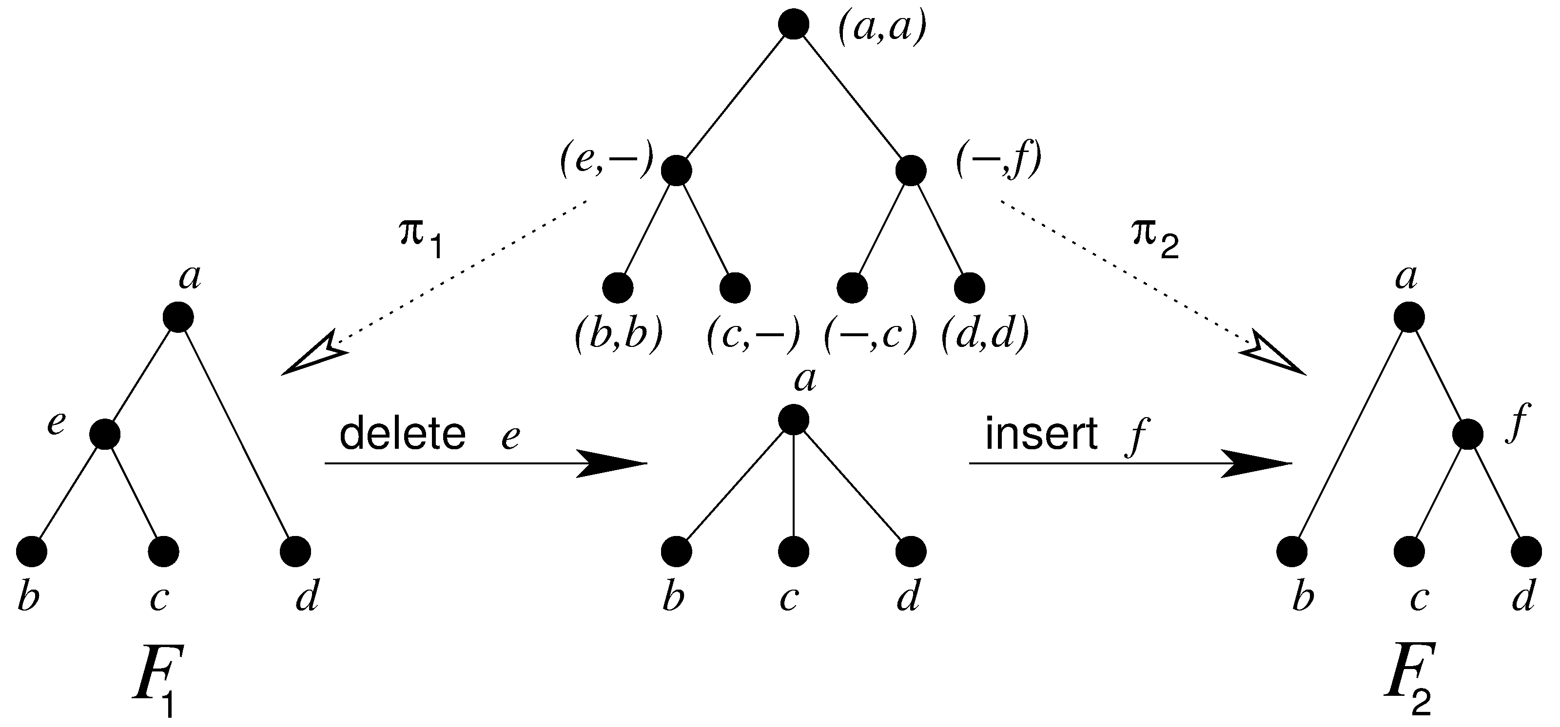
As examples for DP algorithms on trees and forests, we will use the following sections to describe two important and often-used DP problems on trees, the tree editing [32,40] (Section 9) and tree alignment [41] (Section 6) problems. Tree editing is concerned with finding the optimal edit script that transforms the first input tree into the second input tree. Tree alignment, on the other hand, gives the optimal alignment of two trees with each other, as will be described below in more detail. Figure 3 shows the differences between tree alignment and tree editing of two trees and . Tree alignment will find an optimal consensus tree (top) whereas tree editing will find the least number of edit operations in order to transform one tree into the other (bottom). Hence, tree alignment conserves the original structure of both trees opposite to tree editing. More details will be explained in Section 6 and Section 9, respectively. These algorithms serve as a tutorial on how grammars on trees are to be formulated. We expand on earlier work by introducing several variants. While some are known from previous work [17,28,29], the terse and high level notation, ability to construct combined grammars, and automatic derivation of the corresponding outside grammar give a unique framework. Here, we also include some notations on multi-tape DP.
6. Tree Alignment
Our grammar for the case of tree alignment is based on the grammars formulated in [42,43]. We expand those grammars with explicit tree concatenation operators as shown in the previous section. This allows our algorithms to parse both trees and forests as input structures.
Furthermore, we extend the grammars with the automatic derivation of an outside algorithm [24], described in Section 8. The combination of the inside and outside grammar allows for easy calculation of match probabilities. Since this is automatic, any user-defined grammar can be extended in this way as well. Though we point out that this still requires careful design of the inside grammar [7].
Representations of alignments (cf. Figure 3) are typically in the form of a tree that includes nodes from both trees, where matching nodes are given as a pair and deleted nodes from both trees are inserted in a partial-order preserving fashion.
Definition 9 (Tree alignment).
Consider a forest G with vertex labels taken from with as alphabet. Then we obtain mappings and by considering only the first or the second coordinate of the labels, respectively, and by then deleting all nodes that are labeled with the gap character ‘−’, see Figure 3. G is an alignment of the two forests and if and .
The cost of the alignment G based on the original forests and is the sum of the costs based on the labels in G as formulated in Equation (5). Each label consists of a pair of labels , whereas corresponds to a label in the vertex set of or a gap symbol ‘−’ and analogously for .
Every alignment G defines unique mappings and , but the converse is not true. The minimum cost alignment is in general more costly than the minimum cost edit script.
We will need a bit of notation. Let F be an ordered forest. By we denote the subforest consisting of the first i trees, while denotes the subforest starting with the -st tree. By we denote the forest consisting of the children-trees of the root of the first tree in F. is the forest of the right sibling trees of F.
Now consider an alignment A of two forests and . Let be the root of its first tree. We have either:
- . Then and ; is an alignment of and ; is an alignment of and .
- . Then ; for some k, is an alignment of and , and is an alignment of with .
- . Then ; for some k, is an alignment of and and is an alignment of with .
These three cases imply the following dynamic programming recursion:
with initial condition . The formal grammar underlying this recursion is
It is worth noting that single tape projections of the form make perfect sense. Since − is a parser that always matches and returns an empty string, which in turn is the neutral element of the concatenator this formal production is equivalent to . Hence, it produces a forest F that happens to consist just of a single tree T.
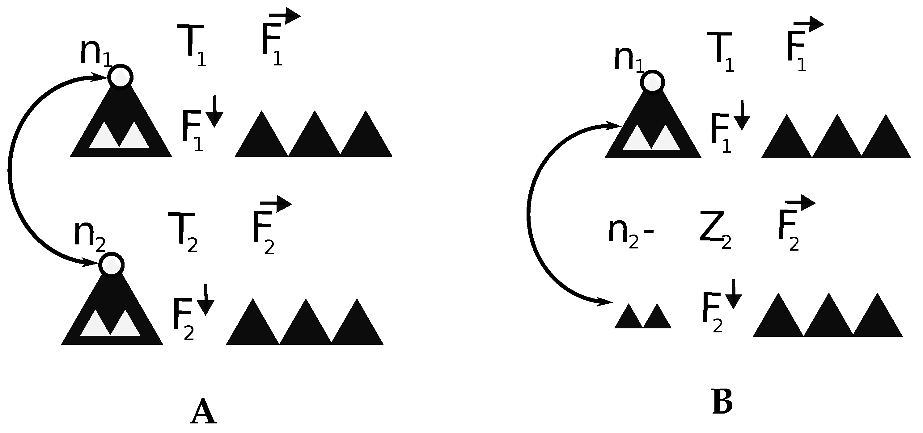
As depicted in Figure 4, fixing the left-most tree T in a forest, there are two directions to traverse the forest: downwards towards the forests of the root’s children and sideways towards the remaining forest . Regarding one single forest, the subforests and are two disjoint entities, thus once split, they do not share any nodes in a further step of the decomposition algorithm. The grammar for tree alignment as described above is inefficient, however, because there is no explicit split between and in the first step. The grammar shown in Equation (8) explicitly splits the two forests in an earlier step to avoid redundancy.
An efficient variant that makes use of a number of facts that turn this problem into the equivalent of a linear grammar on trees has been described [44]. Trees are separated from their forests from left to right, and forests are always right-maximal. Given a local root node for the tree, and a ternary identifier ({T,F,E}), each forest, tree, and empty forest can be uniquely identified. Trees by the local root, forests by the local root of their left-most tree, and empty forests by the leaves “above” them. The asymptotic running time and space complexity for trees with m and n nodes respectively is then . This also holds for multifurcating trees as the decomposition rules do not care if the tree is a binary tree or not. The children of a node in a tree always form a forest, independent of the number of children.
If the nodes of the tree are labelled in pre-order fashion several operations on the forest can be done more efficiently. By splitting a forest into a tree and the remaining forest, we need to store the tree’s indices to know where it is located in the forest. In case of a pre-order indexing we can take the left-most tree without storing additional indices as the left border of the tree is the smallest index (which is its root) of the original forest and the right border of the tree is just the predecessor of the left-most root of the remaining forest. Thus, storing the roots’ indices in a forest will directly give us the right-most leaves of the corresponding trees.
We finally consider a variant of Equation (7) that distinguishes the match rule with a unique non-terminal on the left-hand side of Equation (8). This rule, which corresponds to the matching of the roots of two subtrees, is critical for the calculation of match probabilities and will play a major role in Section 8. The non-terminals and designate insertion and deletion states, respectively. Thus, we can formulate the formal grammar for tree alignment as follows:
This grammar explicitly splits and by applying iter. Hence, these parts recurse independently from each other. As shown in Figure 4, aligning two trees can lead to aligning the downwards forest of one tree to the forest to the right of the other tree. Given Equation (6), the first case corresponds to our first rule in iter and the align rule. Thus replacing in iter we obtain . Here, will give the score for aligning two non-terminals thus . The tree concatenation operators and correspond to and , respectively. Replacing and in the deletion and insertion rules, we get and . This corresponds to case 2 and 3 in Equation (6). As depicted in Figure 4, given a deleted root in one tree, we recurse by aligning both subforests. In case one of the subforests is empty, it will be replaced by the first tree (the first k trees, respectively) of the remaining forest.
The following shows an example scoring algebra for the case of tree alignment with linear gap costs. No costs are added in the iter case but scores obtained from subsolutions are added, given by and . Here, U and V stand for the non-terminal characters whereas are terminals.
Two and Multi-Tape Tree Alignment
Definition 10 (multiple tree alignment).
Let be ordered trees following Definition 1. The partial order of nodes of each tree sorts parent nodes before their children and children are ordered from left to right. An alignment between trees is a triple of functions with defines a function matching nodes in tree to the consensus tree of the alignment:
(i) The set of matched nodes form a partial order-preserving bijection. That is, if are matched with the partial orders and hold for all nodes and pairs of trees . (ii) The set of deleted nodes form a simple surjection from a node onto a symbol (typically ‘-’) indicating no partner. (iii) For trees , (ii) holds analogously.
The problem descriptions in Definitions 9 and 10 are equivalent. Every forest can be defined as a tree with the roots of the forest as children of a trees’ root. Given Definition 9, the mappings and can therefore be applied to a tree as well.
Given Definition 10 (i), the partial order is also preserved in case of forests, as the roots of the forests are partially ordered, too. Definition 10 (ii) and (iii) define the order of the deleted nodes that is preserved within the tree. This is also true for forests, and obtained by the mappings and defined in Definition 9.
A multiple alignment of forest structures can be constructed given the Definitions 2–7 and Lemmas 1 and 2 We now show that, given these definitions, the alignment is well-defined and can always be constructed independent of the input structures. We do not show here that the resulting alignment is optimal in some sense, as this depends on the optimization function (or algebra) used.
Let be an input of k forests. Successive, independent application of the operations specified in Definitions 2–7 and Lemmas 1 and 2 to individual input trees yields the multi-tape version of the empty string , i.e., the input is reduced to empty structures. Not every order of application necessarily yields an alignment.
Just as in the case of sequence alignments [17] the allowed set of operations needs to be defined for multi-tape input. This amounts in particular to specify which operations act concurrently on multiple tapes. The above-given definitions can be subdivided into two sets. One set of operations takes a forest F and splits off the left- or right-most tree ( or ), where both and T are allowed to be empty. In case of T being empty then it holds that . If is empty, then this yields a decomposition of F only if F consists of just a single tree. The other set of operations removes atomic elements from a tree and yields a tree or forest, depending on the rule used.
As in [17], all operations have to operate in “type lockstep” on all inputs simultaneously. That is, either all inputs separate off the left- or right-most tree and yield the trees and remaining forests , or all operations remove a terminal or atomic element, yielding the terminal elements and remaining structure .
Furthermore, an operation ‘−’ is introduced. This operation does not further decompose T but provides a terminal symbol ‘−’ as element . This is analogous to the in/del case in string alignments.
Theorem 1 (Alignment).
Every input of forests can be deconstructed into by successive application of the steps outlined above.
Proof of Theorem 1.
At least one of the decompositions defined above for forests (Definitions 2, 6 and 7) or trees (Definitions 2–5) can always be applied for each input. Due to lockstep handling, all inputs simultaneously separate into a tree and remaining forest (yielding two structures), or apply a rule yielding a terminal element. As such, either all structures are already empty () or at least one structure can be further decomposed yielding a smaller structure.
7. The Affine Gap Cost Model for Alignments
The simple linear scoring of gaps in alignments as in the original formulation by Needleman-Wunsch [26] is often a poor model in computational biology. Instead, one typically uses affine gap cost with a large contribution for opening a gap and small contributions for extending the gaps. The sequence alignment problem with affine gap costs was solved by [45]. The corresponding formal grammar, which is based on the notation in [45] and in the version used by [17], reads
where u and v are terminal symbols, ‘−’ denotes the opening of a gap, and ‘.’ denotes the extension of a gap, typically scored differently. Considering only one tape or input dimension, a deletion is denoted by a leading ‘−’ followed by a number of ‘.’ characters, e.g., a sequence ‘’.
The sequence alignment problem with linear gap costs assumes a constant score for each inserted gap symbol ‘−’. This is not a very realistic assumption for biological sequences, however [46], where sequence intervals are often inserted or deleted as a unit. Hence, affine gap costs, i.e., a larger penalty for the insertion of the first gap symbol than for the extension of an already existing gap, are commonly used in this field. Consequently, algorithms prefer to insert longer connected gap regions than many singletons.
For trees, gap extensions can happen in two directions as a node in a tree has siblings as well as children that are successors given the index structure. Once a node has been aligned to an initial gap symbol (‘−’) both its siblings and its children are extending the initial gap. Compared to the three rules for matching, deletion and insertion, we now have to deal with seven different cases. In [42,43] seven rules for affine gap costs in forests are formulated based on different modes of scoring: no-gap mode, parent-gap mode and sibling-gap mode. Parent and sibling mode indicate that the preceding node (either parent or sibling node) was considered a deletion. The formal grammar expressing the seven rules for tree alignment with affine costs is shown in the Appendix A.
The grammar for tree alignment with affine gap costs in Equation (11) distinguishes between horizontal and vertical gap extension, corresponding to siblings and children in the tree. is the start symbol. Here, we either align the left-most trees or add a gap in one of the roots. Adding a gap in one of the roots leads to a gap extension in the horizontal case, hence and in the vertical case, thus . The rules on the right-hand side for and are the same, as is a forest, too. However, represents a state where the previous node included a gap symbol. Thus, each gap that is added in the next step will be scored with the gap extension score. For the case , no gap was inserted in the direct predecessors, hence every gap added in the next step will be scored with the gap opening score. The grammar was developed in several steps, starting from a larger set of rules and stepwise summarizing rules that are equivalent. An intermediate and larger grammar describing tree alignment with affine gap costs can be found in the Appendix B.
8. Inside and Outside Grammars
The grammars we defined in previous sections are considered as inside grammars in the DP terminology. Inside grammars can be used to calculate two kinds of results. As we have seen above, a globally optimal solution for optimization problems, say the alignment distance between two trees, can be obtained. Alternatively, the partition function can be computed. Here, the sum runs over all configurations , is the score of and is a scaling parameter. For , just counts the number of optimal solutions, for , all conformations are treated equally. The partition function thus provides access to a probabilistic model. This view plays a key role in practical applications.
As described e.g., in [5], the inside-outside algorithm for context-free grammars is analogous to the forward-backward algorithm for HMMs. The inside or forward part calculates the probability for a possible (sub)solution whereas the outside part calculates all possible solutions while keeping one (sub)solution fixed. In this way, it is possible to calculate the overall probability of, e.g., two nodes being aligned to each other in an alignment of two trees. To this end, one calculates the partition function that gives a value for two nodes being matched and the partition function for all possible cases of the complete alignment where those two nodes match. The desired probability is then the ratio of the constrained and the unconstrained partition functions.
In order to know which cases have to be calculated to obtain probabilities for possible (sub)solutions, an Outside grammar can be formulated. The Outside grammar usually has more rules than the Inside grammar and is more complex. In particular, it involves additional non-terminals such as that can be conceptualized as referring to complements of non-terminals of the inside grammar. Its productions specify how the outside object on the left-hand side can be decomposed. In general, the r.h.s. of the productions contain another outside non-terminal as well as inside terminals and non-terminals. The inside objects are the ones that are currently kept fixed wheres the outside objects on the right-hand side define the parts that are used to calculate all possible (sub)solutions with the inside object being fixed. For a detailed discussion of the relationship of Inside and Outside grammars we refer to [24]. Below, we give the outside grammar in Equation (12) (with start symbol , and outside “epsilon” symbols —given that in an outside grammar terminates with full input, not the empty input) for the simple linear-cost tree alignment problem (Equation (12)) and combine inside and outside grammar to yield match probabilities.
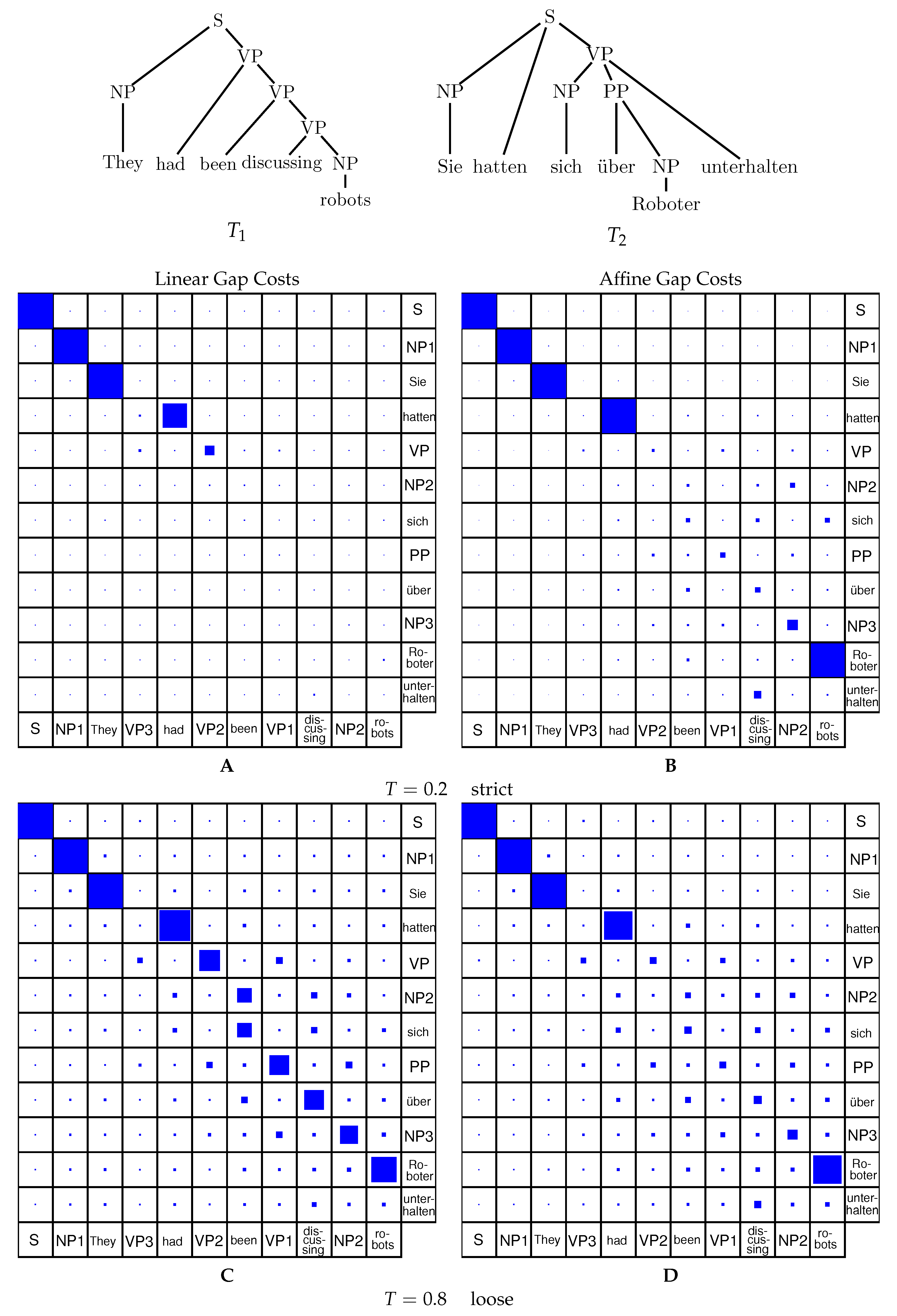
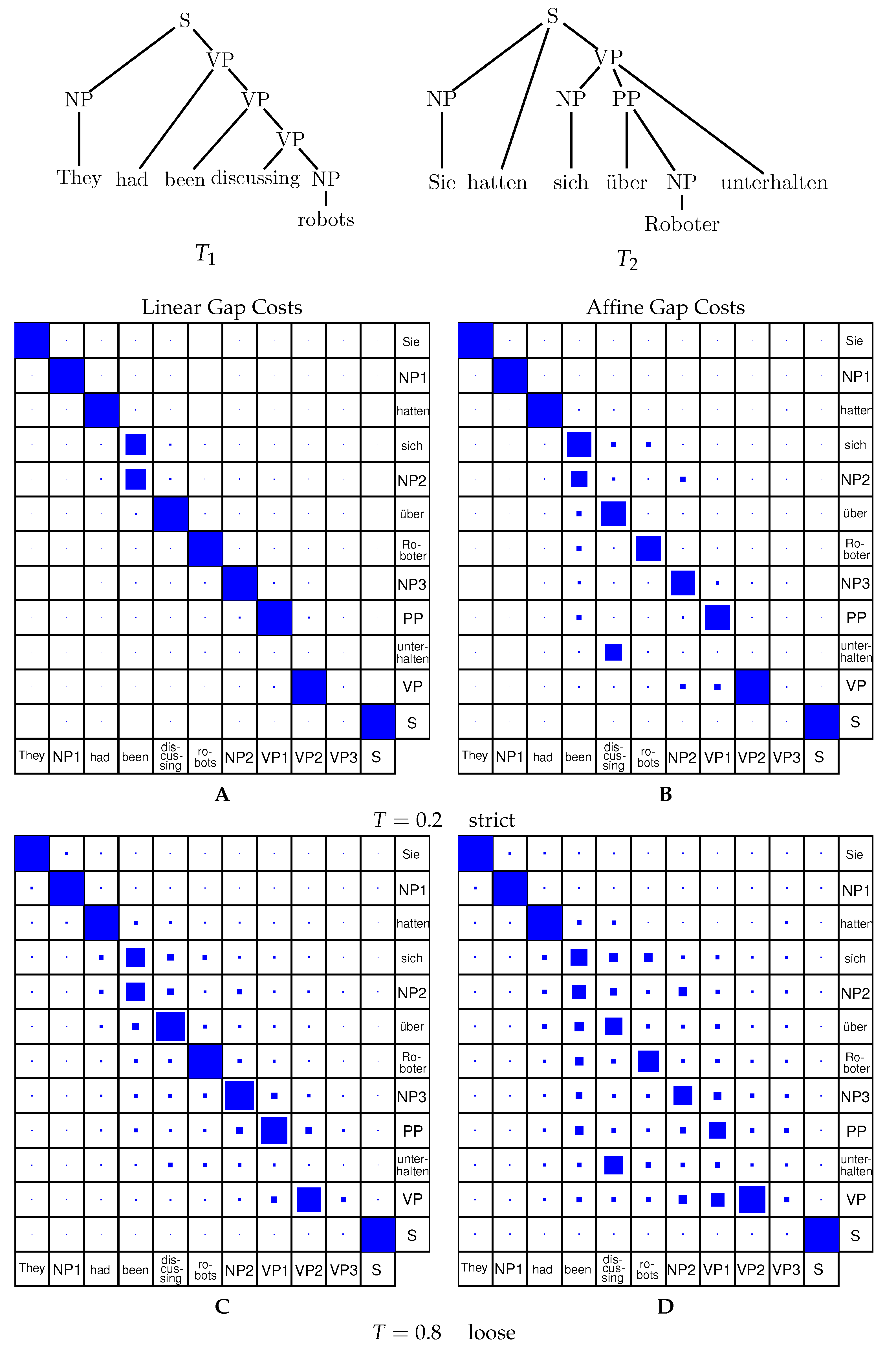
Inside-Outside Algorithm for Affine Gap Costs. The combined Inside-Outside algorithm with an affine gap cost model can be implemented in complete analogy to the linear model. One usually designs the inside grammar based on the recursion equations and the outside grammar is constructed automatically. This yields an algorithm that computes the match probabilities using the affine gap cost model. The example in Figure 5 shows the effect of the scaling parameter T.
Due to the small size of the inputs, alignment with linear and affine gap costs produces similar results. Depending on the scaling parameter, the alignment with the single highest probability mass will dominate ( small) or many sub-optimal solutions will show up with significant probability ( large). For higher scaling parameters, the cost of opening a gap becomes less pronounced yielding a much less constrained probability space than for low values of the scaling parameter—or the linear model with high values for the scaling parameter.
9. Tree Editing
The string-to-string correction problem can be generalized to forests. To this end, edit operations need to be explained for trees. We consider substitution, insertion, and deletion:
![Algorithms 10 00135 i001]() and associate them with costs , , or .
and associate them with costs , , or .

In this section, we explain our formal grammar for the string editing algorithm on trees instead of strings. Comparing and editing strings is a well-known algorithm in computer science applications, and hence, we expanded this application to trees as input described by a formal grammar.
Our grammar is based on [8] which shows one possible solution for the tree editing DP algorithm. There exist other ways which try to minimize the search space of possible solutions by explicitly choosing where to start the next iteration step [31,47,48].
Definition 11 (Tree editing).
A mapping [49] between two ordered forests to is a binary relation between the vertex sets of the two forests such that for pairs holds
- 1.
- if and only if . (one-to-one condition)
- 2.
- x is an ancestor of if and only if y is an ancestor of . (ancestor condition)
- 3.
- x is to the left of if and only if y is to the left of . (sibling condition)
The one-to-one condition implies that for each there is a unique “partner” , i.e., , or x has no matching partner at all. With each mapping we can associate the cost
Individual edit operations correspond to “elementary maps”. Maps can be composed in a natural manner. Thus every edit script corresponds to a map. Conversely every map can be composed of elementary maps, and thus corresponds to an edit script. Furthermore, the cost of maps is subadditive under composition. As a consequence, minimum cost mappings are equivalent to the minimum cost edit scripts [32].
The problem of minimizing has a dynamic programming solution. For a given forest F and a root node v in F, we denote by the forest obtained by deleting v and is the forest obtained from F by deleting with v all descendants of v. Note that is the forest consisting of all trees whose roots are the children of v. Equation (15) shows the recursion equations.
with for two empty forests. A key issue is to implement this algorithm in such a way that only certain classes of subforests need to be evaluated. Our grammar is based on the algorithm described in [8]. Here, forests are decomposed into the right-most tree and the remaining forest, which is not specified in the recursion equations in Equation (15). The corresponding tree editing grammar reads
Note that the empty symbol “−” acts as neutral element for the concatenation operators, which we take to act component-wise. The grammar is based on the tree editing algorithm of [8], for which several more efficient implementations exist. In particular, [50] provides a detailed analysis of the Zhang-Shasha algorithm.
Given the formal grammar (Equation (16)) to the tree editing problem, we modeled the individual cases of the recursion (Equation (15)). Replacing in the iteration rule we get . This matches the third case of the recursion equation, as we add the score for a match and recurse on the forests of the children and the remaining forests. The other two cases of the recursion equation delete the right-most root from one of the current forests using Definition 6, add the score for a deletion or insertion and recurse on the remaining forests.
Tree editing and tree alignment make use of the same decomposition operators and differ only in their formal grammars, index structure and algebras. Many related algorithms on trees, such as the ones described in [51,52], can also be expressed by formal grammars with these decomposition operators. Depending on the details of the problem at hand, the grammar might become more complicated; nevertheless, they usually show striking similarities to the corresponding recursion equations.
9.1. Outside Grammar
Analogously to the outside grammar for tree alignment (Equation (12)), we give the outside grammar for tree editing with start symbol , and outside “epsilon” symbols —given that in an outside grammar terminates with full input, not the empty input.
9.2. Inside-Outside and Affine Gap Costs
The following grammar given in Equation (18) describes tree editing with affine gap costs. Here, non-terminals R and Q describe the gap modes.
Analogous to Figure 5 comparing alignment probabilities for linear and affine gap costs in a strict and a loose case, Figure 6 shows the comparison in the case of tree editing. It can be seen that tree editing generally returns higher probabilities for most of the cases, as tree editing is less strict than tree alignment. This is due to the fact, that deletion and insertion cases for tree editing can freely delete the right-most leaf from the tree while tree alignment will only align root nodes to other root nodes or gap symbols.
10. Benchmarking against RNAforester
RNAforester [44], which is designed to compare RNA secondary structures, is the mostly widely used implementation of tree alignment. In order to compare our Haskell implementation ADPforestry with RNAforester we therefore use RNA secondary structures computed with RNAfold [4] for 50 pairs of RNA sequences of different lengths. The resulting pairs of secondary structures in “dot-bracket” notation together with the RNA sequences directly serve as input for RNAforester. We measured the performance of both programs with both for linear and affine gap costs models. In addition, we show running times for the Inside-Outside (partition function) algorithms implemented in ADPforestry.
Benchmarking results are compiled in Figure 7. Even our prototypical implementation is approximately on par with the performance of RNAforester. ADPforestry at present only implements a simple scoring scheme and none of the elaborate RNA specific scoring schemes provided RNAforester. It also does not attempt to reproduce the detailed, largely RNA-specific output. of RNAforester. In contrast to ADPforestry, RNAforester only solved the optimization version of the tree alignment problem. An alternative implementation of the inside/outside algorithms to compute the a posteriori probabilities of all possible alignment edges is not available at all.
The comparably large effort for the caculation of probabilities is explained by (a) the computation of not only the inside recursion as in case of optimization but also of the corresponding, automatically generated outside recursion, and (b) the fact that the outside recursion is more complex than the inside recursion. Here the inside grammar for tree alignment with linear costs contains 6 rules whereas the corresponding outside grammar is composed of 8 rules. For the affine case, the inside grammar has 16 rules, the outside grammar 25.
11. Implementation
Now that all required theory is in place, we turn toward a prototypical implementation. During the exposition we make several simplifications that are not present in the actual implementation. We also suppressed all references to monadic parametrization. The entire framework works for any monad, giving a type class class (Monad m) => MkStream m x i below. While this is powerful in practice, it is not required in the exposition. As such, the MkStream type class will be presented simply as MkStream x i.
Ordered forests are implemented as a set of vectors instead of using the more natural recursive structure in order to achieve asymptotically better access.
data TreeOrder = Pre | Post
data Forest (p :: TreeOrder) a where
  Forest
    { label     :: Vector a
    , parent    :: Vector Int
    , children  :: Vector (UVector Int)
    , lsib      :: Vector Int
    , rsib      :: Vector Int
    , roots     :: Vector Int
    } -> Forest p a
Each node has a unique index in the range
, and is associated with a label of type a, a parent, a vector of children, and its left and right sibling. In addition, we store a vector of roots for our forest. The Vector data type is assumed to have an index operator (!) with constant time random access. Forests are typed as either being in pre-order or post-order sorting of the nodes. The linear grammars presented beforehand make direct use of the given ordering and we can easily guarantee that only inputs of the correct type are being handled. The underlying machinery for tree alignments is more complex and our choice for an example implementation in this paper. The implementation for tree edit grammars is available in the sources.
Tree Alignment. The tree alignment grammar is a right-linear tree grammar and admits a running time and space optimization to linear complexity for each tape. The grammar itself has been presented in Section 6. Here, we discriminate between three types of sub-structures within a forest via
data TF = T | F | Ewhich allows a forest to be tagged as empty (E) at any node k, be a single tree T with local root k, or be the subforest F starting with the left-most tree rooted at k and be right-maximal. We can thus uniquely identify sub-structures with the index structure
data TreeIxR a t = TreeIxR (Forest Pre a) Int TFfor right-linear tree indices, including the Forest structure introduced above. The phantom type t allows us to tag the index structure as being used in an inside (I) or outside (O) context.
Since the Forest structure is static and not modified by each parsing symbol, it is beneficial to separate out the static parts. ADPfusion provides a data family for running indices RunIx i to this end. With a new structure,
data instance RunIx (TreeIxR (Forest Pre a) I) = Ix Int TFwe capture the variable parts for inside grammars. Not only do we not have to rely on the compiler to lift the static Forest Pre a out of the loops but we also can implement a variant for outside indices with
data instance RunIx (TreeIxR (Forest Pre a) O)
 = Ix Int TF Int TF
Outside index structures need to carry around a pair of indices. One (Int,TF) pair captures index movement for inside tables and terminal symbols in the outside grammar, the other pair captures index movement for outside tables.
Regular shape-polymorphic arrays in Haskell [53] provide inductive tuples. An inductive tuple (Z:.Int:.Int) is isomorphic to an index in
, with Z representing dimension 0, and (:.) constructs inductive tuples. A type class Shape provides, among others, a function toIndex of the index type to a linear index in
. We make use of an analogous type class (whose full definition we elude) that requires us to implement both a linearIndex and a size function. The linear index with largest (
) and current (
) index in the forest
linearIndex (TreeIxR _ u v) (TreeIxR _ k t)
  = (fromEnum v + 1) * k + fromEnum t
and size function
size (TreeIxR _ u v) = (fromEnum v + 1) * (u+1)together allow us to define inductive tuples with our specialized index structures as well. linearIndex and size are defined for the tuple constructor (a:.b) and combine both functions for a and b in such a way as to allow us to write grammars for any fixed dimension.
Parsing with Terminal Symbols. In a production rule of the form
, terminal symbols, denoted t perform the actual parsing, while non-terminals (L, R) provide recursion points (and memoization of intermediate results).
For tree grammars, three terminal symbols are required. The $-parser is successful only on empty substructures, the deletion symbol (−) performs no parse on the given tape, while only the Node parser performs actual work. The first two parsers can be constructed easily, given a node parser. Hence, we give only its construction here.
First, we need a data constructor
data Node r x where
  Node (Vector x -> Int -> r) (Vector x) -> Node r x
that allows us to define a function from an input vector with elements of type x to parses of type r, and the actual input vector of type x. While quite often , this generalization allows to provide additional context for the element at a given index if necessary. We can now bind the labels for all nodes of given input forest f to a node terminal:
let node frst = Node (!) (label frst)where (!) is the index operator into the label vector.
Construction of a Parser for a Terminal Symbol. Before we can construct a parser for a rule such as
, we need a bit of machinery in place. First, we decorate the rule with an evaluation function (f) from the interface (see Section 2), thus turning the rule into
. The left-hand side will not play a role in the construction of the parser as it will only be bound to the result of the parse.
For the right-hand side we need to be able to create a stream of parses. Streams enable us to use the powerful stream-fusion framework [54]. We will denote streams with angled brackets <x> akin to the usual list notation of [x] in Haskell. The elements x of our parse streams are complicated. The element type class
class Element x i where
  data Elm x i :: *
  type Arg x   :: *
  getArg :: Elm x i -> Arg x
  getIdx :: Elm x i -> RunIx i
allows us to capture the important structure for each symbol in a parse. For the above terminal symbol Node we have
instance (Element ls i) => Element (ls , Node r x) i where
  data Elm (ls,Node r x) i = ENd r (RunIx i) (Elm ls i)
  type Arg (ls,Node r x)   = (Arg ls , r)
  getArg (ENd x _ ls)      = (getArg ls , r)
  getIdx (ENd _ i _ )      = i
Each Elem instance is defined with variable left partial parses (ls) and variable index (i) as all index-specific information is encoded in RunIx instances.
Given a partial parse of all elements to the left of the node symbol in ls, we extend the Elm structure for ls inductively with the structure for a Node. The Haskell compiler is able to take a stream of Elm structures, i.e., <Elm x> and erase all type constructors during optimization. In particular, the data family constructors like ENd are erased, as well as the running index constructors, say Ix Int TF. This means that
Elm (ls, Node r x) (RunIx (TreeIxR (Forest Pre a) t))has a runtime representation in a stream fusion stream that is isomorphic to (r,(Int,TF),ls) and can be further unboxed, leading to efficient, tight loops. In case forest labels are unboxable r will be unboxed as well. The recursive content in ls receives the same treatment, leading to total erasure of all constructors.
The MkStream type class does the actual work of turning a right-hand side into a stream of elements. Its definition is simple enough:
class MkStream x i where
  mkStream :: x -> StaticVar -> i -> <Elm x i>
Streams are to be generated for symbols x and some index structure i. Depending on the position of x in a production rule, it might be considered static – having no right neighbor, or variable. In
we have D in variable and R in static position. data StaticVar = Static | Var takes care of this below.
We distinguish two types of elements x for which we need to construct streams. Non-terminals always produce a single value for an index i, independent of the dimensionality of i. Terminal symbols need to deconstruct the dimension of i and produce independent values (or parses) for each dimension or input tape.
Multi-tape Terminal Symbols. For terminal symbols, we introduce yet another inductive tuple, (:|) with zero-dimensional symbol M. We can now construct a terminal that parses a node on each tape via M :| Node (!) i1 :| Node (!) i2. The corresponding MkStream instance hands off work to another type class TermStream for tape-wise handling of each terminal:
instance (TermStream (ts:|t) => MkStream (ls , ts:|t) i
  where mkStream (ls , ts:|t) c i
          = fromTermStream
          . termStream (ts:|t) c i
          . prepareTermStream
          $ mkStream ls i
The required packing and unpacking is performed by fromTermStream and prepareTermStream, and the actual handling is done via TermStream with the help of a type family to capture each parse result.
type family   TArg x :: *
type instance TArg M = Z
type instance TArg (ts:|t) = TermArg ts :. TermArg t
class TermStream t s i where
  termStream :: t -> StaticVar -> i -> <(s,Z,Z)> -> <(s,i,(TArg t))>
Now, we can actually implement the functionality for a stream of Node parses on any given tape for an inside (I) tree grammar:
instance TermStream (ts :| Node r x) s (is:.TreeIxR a I)
where
  termStream (ts:|Node f xs) (_both) (is:.TreeIxR frst i tfe)
  = map (\(s, ii, ee) ->
      let Ix l _ = getIndex s (Proxy :: Proxy (RunIx (is:.TreeIxR a I)))
          l’ = l+1
          ltf’ = if null (children frst ! l) then E else F
      in (s, (ii:.Ix l’ ltf’) (ee:.f xs l)))
  . termStream ts is
  . staticCheck (tfe == T)
We are given the current partial multi-tape terminal state (s,ii,ee) from the left symbol (s), the partial tape index for dimensions 0 to the current dimension
(ii), and parses from dimension 0 up to
(ee).
Then we extract the node index l via getIndex. getIndex makes use of the inductive type-level structure of the index (is:.TreeIxR a I) to extract exactly the right index for the current tape. Since all computations inside getIndex are done on the type level, we have two benefits: (i) it is incredibly hard to confuse two different tapes because we never match explicitly on the structure is of the inductive index structure for the previous
dimensions. (ii) the recursive traversal of the index structure (is:.TreeIxR a I) is a type-level operation. The runtime representation is just a set of unboxed parameters of the loop functions. This means that getIndex is a runtime “no-op” since there is no structure to traverse.
For a forest in pre-order, the first child of the current node l is just
. In case of a node without children, we set this to be empty (E), and otherwise we have a forest starting at
. We then extend the partial index ii to include the index for this tape, and analogously extend the partial parse ee with this parse.
Non-Terminals. Streams are generated differently for non-terminals. A non-terminal captures the parsing state for a complete (multi-dimensional) index, not for individual tapes. The ITbl i x data type captures memoizing behaviour for indices of type i, and memoized elements of type x. One may consider this data type to behave essentially like a memoizing function of type
. We can capture this behaviour thus:
instance (Elem ls i) => Elem (ls, ITbl i x) i where
  data Elm (ls, ITbl i x) i = EIt x (RunIx i) (Elm ls i)
  type Arg (ls, ITbl i x)   = (Arg ls, r)
  getArg (EIt x _ ls)       = (getArg ls, r)
  getIdx (EIt _ i _ )       = i
instance MkStream (ls, ITbl (is:.i) x) (is:.i) where
  mkStream (ls, ITbl t f) ix
    = map ((s,tt,ii) -> ElmITbl (t!tt) ii s)
    . addIndexDense ix
    $ mkStream ls ix
Again, we require the use of an additional type class capturing addIndexDense. In this case, this makes it possible to provide n different ways on how to memoize (via ITbl for dense structures, IRec if no memoization is needed, etc.) with m different index types using just
instances instead of
.
class AddIndexDense i where
  addIndexDense :: i -> <s Z> -> <s i>
Indexing into non-terminals can be quite involved however, and tree structures are no exception. A production rule
splits a forest into the tree-like element D that is explored further downwards from its local root, and the remaining right forest R. Both D and R can be in various states. These states are
data TFsize s = EpsFull TF s | FullEps s | OneRem s
              | OneEps s | Finis
In the implementation below, the optimizer makes use of constructor specialization [55] to erase the TFsize constructors, while they allow us to provide certain guarantees of having captured all possible ways on how to partition a forest.
Excluding Finis, which denotes that no more parses are possible, we consider four major split operations:
-
EpsFull denotes an empty tree D meaning that the “left-most” element to be aligned to another subforest will actually be empty. This will later on induce a deletion on the current tape, if an empty D needs to be aligned to a non-empty structure.
-
FullEps will assign the complete remaining subforest to D, which will (obviously) not be a tree but a forest. While no tree (on another tape) can be aligned to a forest, the subforest below a tree on another tape can be aligned to this forest.
-
OneRem splits off the left-most tree to be bound to D, with the remaining siblings (the tail) being bound to R.
-
Finally, OneEps takes care of single trees masquerading as forests during a sequence of deletions on another tape.
All the logic of fixing the indices happens in the variable case for the D non-terminal. The static case for R just needs to extract the index and disallow further non-terminals from accessing any subforest as all subforests are right-maximal.
instance AddIndexDense (is:.TreeIxR a I) where
  addIndexDense (vs:.Static) (is:.TreeIxR _ _ _)
  = map go . addIndexDense vs is where
    go (s,tt,ii) =
      let t = getIndex s (Proxy :: Proxy (RunIx (is:.TreeIxR a)))
      in (s, tt:.t, ii:.Ix maxBound E)
-- continued below
In the variable case, we need to take care of all possible variations. The use of flatten to implement “nested loops” in Haskell follows in the same way as in [18]. Done and Yield are stream fusion step constructors [54] that are explicit only in flatten.
-- continued
 addIndexDense (vs:.Variable) (is:.TreeIxR f j tj)
 = flatten mk step . addIndexDense vs is where
 mk = return . EpsFull jj
-- forests
 step (EpsFull E (s,t,i))
   = Yield (s, t:.TreeIxR f j E, i:.Ix j E) Finis
 step (EpsFull F (s,t,i))
   = let Ix k _ = getIndex s (Proxy :: Proxy (RunIx (is:.TreeIxR a)))
   in Yield (s, t:.TreeIxR f k E, i:.Ix k F) (FullEps (s,t,i))
 step (FullEps (s,t,i))
   = let Ix k _ = getIndex s (Proxy :: Proxy (RunIx (is:.TreeIxR a)))
         u = maxBound
   in Yield (s, t:.TreeIxR f k F, i:.Ix u E) (OneRem (s,t,i))
 step (OneRem (s,t,i))
   = let Ix k _ = getIndex (Proxy :: Proxy (RunIx (is:.TreeIxR a)))
         l = rightSibling f k
   in Yield (s, t:.TreeIxR f k T, i:.Ix l F) Finis
-- trees
 step (EpsFull T (s,t,i))
   = let Ix k _ = getIndex (Proxy :: Proxy (RunIx (is:.TreeIxR a)))
   in Yield (s,tt:.TreeIxR f k E,ii:.Ix k T) (OneEps (s,t,i))
 step (OneEps (s,t,i))
   = let Ix k _ = getIndex (Proxy :: Proxy (RunIx (is:.TreeIxR a)))
   in Yield (s,tt:.TreeIxR f k T,ii:.Ix k E) Finis
rightSibling :: Forest -> Int -> Int
rightSibling f k = rsib f ! k
This concludes the presentation of the machinery necessary to extend ADPfusion to parse forest structures. The full implementation includes an extension to Outside grammars as well, in order to implement the algorithms as described in Section 8. We will not describe the full implementation for outside-style algorithms here as they require some effort. The source library has extensive annotations in the comments that describe all cases that need to be considered.
The entire low-level implementation given above can remain transparent to a user who just wants to implement grammars on tree and forest structures since the implementation works seamlessly together with the embedded domain-specific languages ADPfusion [18] and its abstraction that uses a quasi-quotation [56] mechanism to hide most of this more intermediate-level library.
12. Conclusions
Tree comparison has many applications and there exist several approaches in the literature that optimize exisiting algorithms based on the size of the search space or time and memory requirements. Based on existing optimizations, we formalized the algorithms tree editing [8] and tree alignment [42,43] such that they can be written as formal grammars as it has been done for string comparison [17]. Compared to strings, trees can be traversed in two directions, thus our data structure is 2-dimensional. Each grammar consists of terminals and non-terminals, whereas the terminals are single nodes and the non-terminals specify a tree and a forest.
In addition to the linear gap cost version of the algorithms, we developed grammars that provide variants with affine gap costs. Compared to simple, linear cost functions, additional non-terminals are required to distinguish between the initialization of a gap, or gap opening, and gap extension.
For each (inside) grammar, the corresponding outside grammar of the original algorithm [24] can be automatically calculated. Using inside and outside versions, we can specify match probabilities for each pair of subtrees. The inside and outside grammar together thus allow the calculation of ensemble properties such as the probability of each pair of local tree roots to be paired with each other.
For a concrete example from the area of linguistics, we give programs that calculate the pair and editing probabilities for sentences in German and English. While these programs are prototypical and not intended for serious analysis of sentence similarities between languages, they already provide information on conserved sentence structure.
In addition they show how the inclusion of affine costs modifies the observed behaviour. This leads to one of the major points of our framework: trying a variant, such as affine costs for tree alignment including Inside-Outside calculations can now be done with sufficient ease to allow for exploration of the “space of grammars” that describe a problem instance well.
Combining ADP with tree and forest structures as input, we are now able to apply single-tape and multi-tape DP algorithms on tree-like data. Together with the inclusion of Inside-Outside algorithms, the search space of DP algorithms on trees and forests can be explored broadly. As grammar and algebra can be changed easily, it is possible to compare results based on distinct grammars or cost functions.
One area we have touched only in passing are extensions of both tree alignment and tree editing beyond two inputs. The basic Definition 10 for tree alignment gives the minimum required structure of an alignment, both alignments and edit scripts for trees deserve further treatment outside of the scope of this work. For sequence-based algorithms, we have a formal framework [17,27] that extends any desired number of sequences and an extension to tree-based algorithms should be investigated.
Further complications arise whenever non-ambiguity is desired. Here, we were mostly concerned with the theoretical basis for a formal language on tree inputs, but as shown by, e.g., [7], the design of a non-ambiguous algorithm on tree inputs is non-trivial. This topic deserves further treatment since proof of non-ambiguity would allow users of our framework to calculate ensemble properties (almost for free thanks to [24,28]) with the knowledge that their underlying algorithm does not overcount certain structures.
Supplementary Materials
Implementations for the algorithms discussed here are available on hackage and github. The ADPfusionForest framework extensions are available here http://hackage.haskell.org/package/ADPfusionSet and prototypical implementations of the forest-based algorithms here http://hackage.haskell.org/package/Forestry. The latter are accompanied by a simple RNAforester variant.
Acknowledgments
S.J.B. was supported by DAAD and JSPS (within the JSPS Summer Program 2017). The authors thank the reviewers for helpful comments and hints.
Author Contributions
S.J.B., C.H.z.S. and P.F.S. jointly designed the study and wrote the manuscript. S.J.B. implemented the algorithms and analyzed the data.
Conflicts of Interest
The authors declare no conflict of interest.
Appendix A. Original Grammar for Affine Gap Costs
The following grammer expresses the seven rules for affine gap costs in forests [42,43]. Here, different modes of scoring are applied: no-gap mode, parent-gap mode and sibling-gap mode. Parent and sibling mode indicate that the preceding node (either parent or sibling node) was considered a deletion. Correspondingly, the non-terminal symbol F denotes a no-gap state, P denotes a parent gap, and G denotes a sibling gap. This means that in P mode a gap was introduced in a node further toward the root, while in G mode a gap was introduced in a sibling. In both modes, an unbroken chain of deletions then follows on that tape.
This grammar supports different scoring functions for parent and sibling gaps. Gap opening and gap extension can be distinguished explicitly by including the two additional rules given in Equation (A2). They are useful in particular to produce a more expressive output in the backtracing step.
Appendix B. Intermediary Version of Grammar for Affine Gap Costs
As, in most applications, there is little reason to distinguish the parent and sibling mode gaps in the scoring function. Omitting also the explicit rules for gap extension, the grammar can be simplified considerably, see also [42,43]. Here, denotes the non-gap mode, whereas the gap-mode is represented by mixed terms. In particular, and open gaps, while the remaining mixed terms refer to gap extensions.
The rules for , , and produce the same cases on their right-hand sides. The difference are the l.h.s. cases, which distinguish between no-gap mode and gap mode, thus between affine extension cost and gap opening cost. Additionally, the rules expressing parent gap modes and are recursively calling themselves. Some rules of the grammar can be condensed as they model equivalent cases. The fully compressed version is described in Section 7.
Appendix C. Sankoff’s and Fitch’s Algorithms
Sankoff’s algorithm, and many others often used in particular in computational biology, proceeds using two decomposition steps, namely, the separation of the root from the forest of its child trees, and the stepwise decomposition of a forest into its component trees. The grammar underlying Equation (2) thus is
The same grammar can be use to describe Fitch’s small parsimony problem [35] for binary trees, which was later generalized by Hartigan [36] for arbitrary trees. Even though, both problems, the Sankoff as well as the Fitch/Hartigan algorithm use the same grammar, the evaluation algebras differ significantly. Each scoring algebra consists of functions corresponding to the rules in the grammar, thus in this case, a tree function, a forest function, a function for the empty case together with the choice function form the algebra. Each (sub)solution consists of a list of pairs consisting of the score for the input tree T and a set , containing the nodes included in the solution. Thus, each instance of the problem will also receive the list of pairs as an input. Let A be the set of possible labels in the tree and l the length of the input list. Then Fitch/Hartigan uses the scoring algebra depicted in Figure A1. For the Sankoff version, only a label-dependent score w for the trees is given as input, with as the set of labels in the current subtree T, as it can be seen in Figure A2. Thus, the second algebra considers the Sankoff version of the small parsimony problem.
Figure A1.
Scoring algebra for the Fitch/Hartigan version of the small parsimony problem.
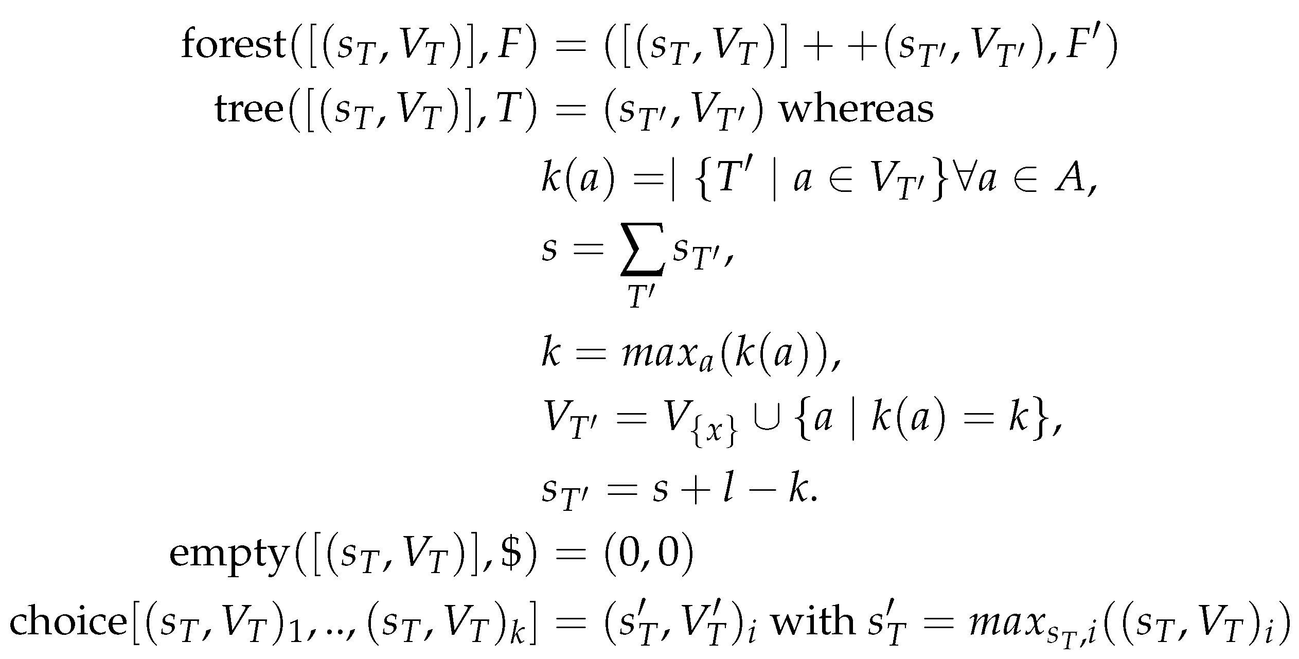
Figure A2.
Scoring algebra for the Sankoff version of the small parsimony problem. Here, is the list of scores for possible (sub)solutions and with a further element is added to the list.
Figure A2.
Scoring algebra for the Sankoff version of the small parsimony problem. Here, is the list of scores for possible (sub)solutions and with a further element is added to the list.
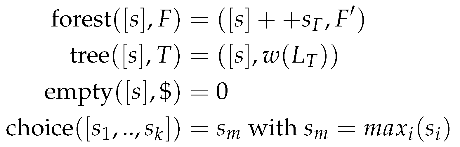
References
- Bellman, R. On the theory of dynamic programming. Proc. Natl. Acad. Sci. USA 1952, 38, 716–719. [Google Scholar] [CrossRef] [PubMed]
- Sankoff, D.; Kruskal, J.B. (Eds.) Time Warps, String Edits, and Macromolecules: The Theory and Practice of Sequence Comparison; Addison-Wesley: Reading, MA, USA; Don Mills, ON, Canada, 1983. [Google Scholar]
- Hofacker, I.L.; Fontana, W.; Stadler, P.F.; Bonhoeffer, L.S.; Tacker, M.; Schuster, P. Fast folding and comparison of RNA secondary structures. Monatshefte für Chemie/Chem. Mon. 1994, 125, 167–188. [Google Scholar] [CrossRef]
- Lorenz, R.; Bernhart, S.H.; Höner zu Siederdissen, C.; Tafer, H.; Flamm, C.; Stadler, P.F.; Hofacker, I.L. ViennaRNA Package 2.0. Algorithms Mol. Biol. 2011. [Google Scholar] [CrossRef] [PubMed]
- Durbin, R.; Eddy, S.R.; Krogh, A.; Mitchison, G. Biological Sequence Analysis: Probabilistic Models of Proteins and Nucleic Acids; Cambridge University Press: Cambridge, UK, 1998. [Google Scholar]
- Felsenstein, J. Evolutionary trees from DNA sequences: A maximum likelihood approach. J. Mol. Evol. 1981, 17, 368–376. [Google Scholar] [CrossRef] [PubMed]
- Chauve, C.; Courtiel, J.; Ponty, Y. Counting, generating and sampling tree alignments. In Proceedings of the International Conference on Algorithms for Computational Biology, Trujillo, Spain, 21–22 June 2016; pp. 53–64. [Google Scholar]
- Zhang, K.; Shasha, D. Simple fast algorithms for the editing distance between trees and related problems. SIAM J Comput. 1989, 18, 1245–1262. [Google Scholar] [CrossRef]
- Jacox, E.; Chauve, C.; Szöllősi, G.J.; Ponty, Y.; Scornavacca, C. ecceTERA: Comprehensive gene tree-species tree reconciliation using parsimony. Bioinformatics 2016, 32, 2056–2058. [Google Scholar] [CrossRef] [PubMed]
- Schirmer, S.; Ponty, Y.; Giegerich, R. Introduction to RNA secondary structure comparison. In RNA Sequence, Structure, and Function: Computational and Bioinformatic Methods; Humana Press: Totowa, NJ, USA, 2014; pp. 247–273. [Google Scholar]
- Rinaudo, P.; Ponty, Y.; Barth, D.; Denise, A. Tree decomposition and parameterized algorithms for RNA structure-sequence alignment including tertiary interactions and pseudoknots. In Proceedings of the 12th Workshop on Algorithms in Bioinformatics (WABI 2012), Ljubljana, Slovenia, 9–11 September 2012; pp. 149–164. [Google Scholar]
- Giegerich, R.; Touzet, H. Modeling Dynamic Programming Problems over Sequences and Trees with Inverse Coupled Rewrite Systems. Algorithms 2014, 7, 62–144. [Google Scholar] [CrossRef] [Green Version]
- Cantor, D.G. On the ambiguity problem of Backus systems. J. ACM 1962, 9, 477–479. [Google Scholar] [CrossRef]
- Floyd, R.W. On ambiguity in phrase structure languages. Commun. ACM 1962, 5, 526–534. [Google Scholar] [CrossRef]
- Brabrand, C.; Giegerich, R.; Møller, A. Analyzing ambiguity of context-free grammars. Sci. Comput. Program. 2010, 75, 176–191. [Google Scholar] [CrossRef]
- Giegerich, R. A systematic approach to dynamic programming in bioinformatics. Bioinformatics 2000, 16, 665–677. [Google Scholar] [CrossRef] [PubMed]
- Höner zu Siederdissen, C.; Hofacker, I.L.; Stadler, P.F. Product Grammars for Alignment and Folding. IEEE/ACM Trans. Comput. Biol. Bioinform. 2015, 12, 507–519. [Google Scholar] [CrossRef] [PubMed]
- Höner zu Siederdissen, C. Sneaking around concatMap: Efficient combinators for dynamic programming. In Proceedings of the 17th ACM SIGPLAN International Conference on Functional Programming, ICFP ’12, Copenhagen, Denmark, 9–15 September 2012; ACM: New York, NY, USA, 2012; Volume 47, pp. 215–226. [Google Scholar]
- Sauthoff, G.; Janssen, S.; Giegerich, R. Bellman’s GAP—A Declarative Language for Dynamic Programming. In Proceedings of the 13th International ACM SIGPLAN Symposium on Principles and Practices of Declarative Programming, PPDP ’11, Odense, Denmark, 20–22 July 2011; pp. 29–40. [Google Scholar]
- Sauthoff, G.; Möhl, M.; Janssen, S.; Giegerich, R. Bellman’s GAP—A Language and Compiler for Dynamic Programming in Sequence Analysis. Bioinformatics 2013, 29, 551–560. [Google Scholar] [CrossRef] [PubMed]
- Brainerd, W.S. Tree generating regular systems. Inf. Control 1969, 14, 217–231. [Google Scholar] [CrossRef]
- Giegerich, R. Code selection by inversion of order-sorted derivors. Theor. Comput. Sci. 1990, 73, 177–211. [Google Scholar] [CrossRef]
- Giegerich, R.; Meyer, C.; Steffen, P. A Discipline of Dynamic Programming over Sequence Data. Sci. Comput. Program. 2004, 51, 215–263. [Google Scholar] [CrossRef]
- Höner zu Siederdissen, C.; Prohaska, S.J.; Stadler, P.F. Algebraic Dynamic Programming over General Data Structures. BMC Bioinform. 2015, 16, S2. [Google Scholar] [CrossRef] [PubMed]
- Giegerich, R.; Meyer, C. Algebraic Dynamic Programming. In Algebraic Methodology and Software Technology; Springer: Berlin/Heidelberg, Germany, 2002; Volume 2422, pp. 243–257. [Google Scholar]
- Needleman, S.B.; Wunsch, C.D. A general method applicable to the search for similarities in the amino acid sequence of two proteins. J. Mol. Biol. 1970, 48, 443–453. [Google Scholar] [CrossRef]
- Höner zu Siederdissen, C.; Hofacker, I.L.; Stadler, P.F. How to Multiply Dynamic Programming Algorithms. In Brazilian Symposium on Bioinformatics (BSB 2013); Lecture Notes in Bioinformatics; Springer: Heidelberg, Germany, 2013; Volume 8213, pp. 82–93. [Google Scholar]
- Höner zu Siederdissen, C.; Prohaska, S.J.; Stadler, P.F. Dynamic Programming for Set Data Types. In Brazilian Sympositum on Bioinformatics (BSB 2014); Lecture Notes in Bioinformatics; Springer: Heidelberg, Germany, 2014; Volume 8826, pp. 57–64. [Google Scholar]
- Riechert, M.; Höner zu Siederdissen, C.; Stadler, P.F. Algebraic Dynamic Programming for Multiple Context-Free Languages. Theor. Comput. Sci. 2016, 639, 91–109. [Google Scholar] [CrossRef]
- Chen, W. New algorithm for ordered tree-to-tree correction problem. J. Algorithms 2001, 40, 135–158. [Google Scholar] [CrossRef]
- Schwarz, S.; Pawlik, M.; Augsten, N. A New Perspective on the Tree Edit Distance. In Proceedings of the International Conference on Similarity Search and Applications, Munich, Germany, 4–6 October 2017; pp. 156–170. [Google Scholar]
- Tai, K.C. The tree-to-tree correction problem. J. ACM (JACM) 1979, 26, 422–433. [Google Scholar] [CrossRef]
- Nussinov, R.; Jacobson, A.B. Fast algorithm for predicting the secondary structure of single-stranded RNA. Proc. Natl. Acad. Sci. USA 1980, 77, 6309–6313. [Google Scholar] [CrossRef] [PubMed]
- Sankoff, D. Minimal mutation trees of sequences. SIAM J. Appl. Math. 1975, 28, 35–42. [Google Scholar] [CrossRef]
- Fitch, W.M. Towards defining the course of evolution: Minimum change for a specific tree topology. Syst. Biol. 1971, 20, 406–416. [Google Scholar] [CrossRef]
- Hartigan, J.A. Minimum mutation fits to a given tree. Biometrics 1973, 29, 53–65. [Google Scholar] [CrossRef]
- Maddison, W.P. Testing Character Correlation using Pairwise Comparisons on a Phylogeny. J. Theor. Biol. 2000, 202, 195–204. [Google Scholar] [CrossRef] [PubMed]
- Arnold, C.; Nunn, C.L. Phylogenetic Targeting of Research Effort in Evolutionary Biology. Am. Nat. 2010, 176, 601–612. [Google Scholar] [CrossRef] [PubMed] [Green Version]
- Arnold, C.; Stadler, P.F. Polynomial algorithms for the Maximal Pairing Problem: Efficient phylogenetic targeting on arbitrary trees. Algorithms Mol. Biol. 2010, 5, 25. [Google Scholar] [CrossRef] [PubMed] [Green Version]
- Selkow, S.M. The tree-to-tree editing problem. Inf. Process. Lett. 1977, 6, 184–186. [Google Scholar] [CrossRef]
- Jiang, T.; Wang, L.; Zhang, K. Alignment of trees – an alternative to tree edit. Theor. Comput. Sci. 1995, 143, 137–148. [Google Scholar] [CrossRef]
- Schirmer, S. Comparing Forests. Ph.D. Thesis, Bielefeld University, Bielefeld, Germany, 2011. [Google Scholar]
- Schirmer, S.; Giegerich, R. Forest alignment with affine gaps and anchors. In Combinatorial Pattern Matching; Springer: Berlin/Heidelberg, Germany, 2011; pp. 104–117. [Google Scholar]
- Höchsmann, M. The Tree Alignment Model: Algorithms, Implementations and Applications for the Analysis of RNA Secondary Structures. Ph.D. Thesis, Technische Fakultät, Universität Bielefeld, Bielefeld, Germany, 2005. [Google Scholar]
- Gotoh, O. An improved algorithm for matching biological sequences. J. Mol. Biol. 1982, 162, 705–708. [Google Scholar] [CrossRef]
- Reese, J.T.; Pearson, W.R. Empirical determination of effective gap penalties for sequence comparison. Bioinformatics 2002, 18, 1500–1507. [Google Scholar] [CrossRef] [PubMed]
- Pawlik, M.; Augsten, N. Tree edit distance: Robust and memory-efficient. Inf. Syst. 2016, 56, 157–173. [Google Scholar] [CrossRef]
- Bringmann, K.; Gawrychowski, P.; Mozes, S.; Weimann, O. Tree Edit Distance Cannot be Computed in Strongly Subcubic Time (unless APSP can). In Proceedings of the SODA 2018, New Orleans, LA, USA, 7–8 January 2018. [Google Scholar]
- Bille, P. A survey on tree edit distance and related problems. Theor. Comput. Sci. 2005, 337, 217–239. [Google Scholar] [CrossRef]
- Dulucq, S.; Tichit, L. RNA secondary structure comparison: Exact analysis of the Zhang-Shasha tree edit algorithm. Theor. Comput. Sci. 2003, 306, 471–484. [Google Scholar] [CrossRef]
- Kan, T.; Higuchi, S.; Hirata, K. Segmental mapping and distance for rooted labeled ordered trees. Fundam. Inform. 2014, 132, 461–483. [Google Scholar]
- Kuboyama, T. Matching and Learning in Trees. Ph.D. Thesis, Gakushuin University, Tokyo, Japan, 2007. [Google Scholar]
- Keller, G.; Chakravarty, M.M.; Leshchinskiy, R.; Peyton Jones, S.; Lippmeier, B. Regular, Shape-polymorphic, Parallel Arrays in Haskell. In Proceedings of the 15th ACM SIGPLAN International Conference on Functional Programming, ICFP ’10, Baltimore, MD, USA, 27–29 September 2010; pp. 261–272. [Google Scholar]
- Coutts, D.; Leshchinskiy, R.; Stewart, D. Stream Fusion: From Lists to Streams to Nothing at All. In Proceedings of the 12th ACM SIGPLAN International Conference on Functional Programming, ICFP ’07, Freiburg, Germany, 1–3 October 2007; pp. 315–326. [Google Scholar]
- Peyton Jones, S. Call-pattern Specialisation for Haskell Programs. In Proceedings of the 12th ACM SIGPLAN International Conference on Functional Programming, ICFP ’07, Freiburg, Germany, 1–3 October 2007; pp. 327–337. [Google Scholar]
- Mainland, G. Why It’s Nice to be Quoted: Quasiquoting for Haskell. In Proceedings of the ACM SIGPLAN Workshop on Haskell Workshop, Freiburg, Germany, 1–3 October 2007; pp. 73–82. [Google Scholar]
Figure 1.
Two different scoring algebras written for the grammar of string alignment. Here, is the score, the input alphabet, − the gap symbol and $ the empty string. The score contributions evaluate the edit operations, here (mis)matches, deletions and insertions, depending on the values of emitted terminal symbols. The choice function formalizes the selection criterion, or objective function applied in each recursion step. In the count algebra (left) it returns the sum of the alternatives. In the eval algebra (right), the choice function h is usually defined as max or min to retrieve the optimal value.
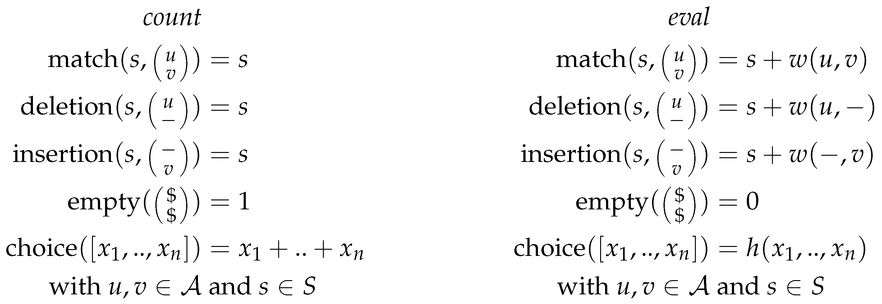
Figure 2.
Signature for the problem of string alignment. The signature lists the situations that need to be evaluated differently by specifying the input and output for each situation. Here, S is the score, a letter from the alphabet, − the none symbol and $ the empty symbol.
Figure 2.
Signature for the problem of string alignment. The signature lists the situations that need to be evaluated differently by specifying the input and output for each situation. Here, S is the score, a letter from the alphabet, − the none symbol and $ the empty symbol.

Figure 3.
Alignment of two forests and (top) and a sequence of edit operations (relabel, delete, insert) in order to transform into (below). Tree alignment conserves the structures of both original trees that can be recovered using the mapping or , respectively. For more details, see Section 6.
Figure 3.
Alignment of two forests and (top) and a sequence of edit operations (relabel, delete, insert) in order to transform into (below). Tree alignment conserves the structures of both original trees that can be recovered using the mapping or , respectively. For more details, see Section 6.

Figure 4.
Alignment of two forests 1 (top) and 2 (bottom). Each of the forests is split into its left-most tree and the remaining forest . (A) The left-most tree will be split into its root nodes and the forests of its children, . (B) In case is deleted, a gap symbol is added and the recursion continues with and .

Figure 5.
Match probabilities for alignments of the trees and for linear (A,C) and affine (B,D) gap costs, and for two different choices of the scaling parameter T, 0.2 (A,B) and 0.8 (C,D). The size of the squares scales logarithmically with the probability as . The score were set to −2 for indels and mismatch, 2 for matches and −1 for the affine gap costs in the affine case. The trees refer to syntax trees for a sentence in German () and in English () as shown above.

Figure 6.
Match probabilities for edits of the trees and for linear (A,C) and affine (B,D) gap costs, and for two different choices of the scaling parameter T, 0.2 (A,B) and 0.8 (C,D). The size of the squares scales logarithmically with the probability as . The scores were set to −2 for indels and mismatch, 2 for matches and −1 for the affine gap costs in the affine case. The trees refer to syntax trees for a sentence in German () and in English () as depicted in the figure. In comparison to the tree alignment case, the labels of the trees’ nodes are in a slightly different order, as tree editing uses postorder while tree alignment is based on trees in preorder.

Figure 7.
Comparison of the running times (in seconds) of RNAforester and algebraic dynamic programming (ADP)forestry measured as an average over 50 instances of random RNA secondary structures of different lengths using linear and affine gap costs, respectively. The benchmarks were performed on an Intel(R) Core(TM) i5-4570 machine with 32 Gb memory. RNAforester does not implement an Inside-Outside (partition function) version of tree alignment.
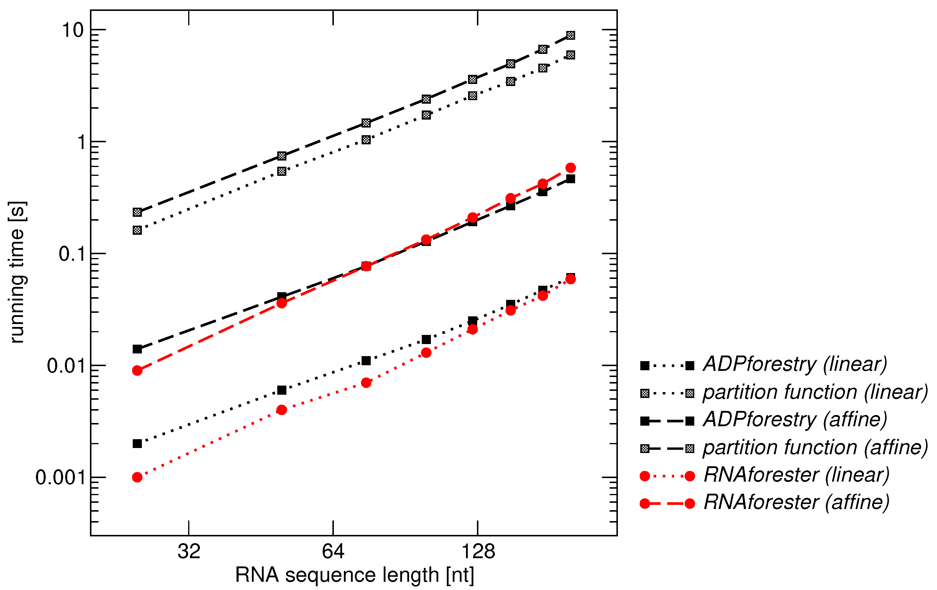
© 2017 by the authors. Licensee MDPI, Basel, Switzerland. This article is an open access article distributed under the terms and conditions of the Creative Commons Attribution (CC BY) license (http://creativecommons.org/licenses/by/4.0/).
Share and Cite
MDPI and ACS Style
Berkemer, S.J.; Höner zu Siederdissen, C.; Stadler, P.F. Algebraic Dynamic Programming on Trees. Algorithms 2017, 10, 135. https://doi.org/10.3390/a10040135
AMA Style
Berkemer SJ, Höner zu Siederdissen C, Stadler PF. Algebraic Dynamic Programming on Trees. Algorithms. 2017; 10(4):135. https://doi.org/10.3390/a10040135
Chicago/Turabian StyleBerkemer, Sarah J., Christian Höner zu Siederdissen, and Peter F. Stadler. 2017. "Algebraic Dynamic Programming on Trees" Algorithms 10, no. 4: 135. https://doi.org/10.3390/a10040135
Note that from the first issue of 2016, this journal uses article numbers instead of page numbers. See further details here.