Weakly Coupled Distributed Calculation of Lyapunov Exponents for Non-Linear Dynamical Systems

Abstract

Numerical estimation of Lyapunov exponents in non-linear dynamical systems results in a very high computational cost. This is due to the large-scale computational cost of several Runge–Kutta problems that need to be calculated. In this work we introduce a parallel implementation based on MPI (Message Passing Interface) for the calculation of the Lyapunov exponents for a multidimensional dynamical system, considering a weakly coupled algorithm. Since we work on an academic high-latency cluster interconnected with a gigabit switch, the design has to be oriented to reduce the number of messages required. With the design introduced in this work, the computing time is drastically reduced, and the obtained performance leads to close to optimal speed-up ratios. The implemented parallelisation allows us to carry out many experiments for the calculation of several Lyapunov exponents with a low-cost cluster. The numerical experiments showed a high scalability, which we showed with up to 68 cores.

1. Introduction

Although the study of non-linear differential equations began with the rise of differential equations themselves, formally, the birth of the modern field of non-linear dynamical systems began in 1962 when Edward Lorenz, a MIT meteorologist, computationally simulated a set of differential equations for fluid convection in the atmosphere. In such simulations, he noticed a complicated behaviour that seemed to depend sensitively on initial conditions, and here he found the “Lorenz” strange attractor. The field of non-linear dynamical systems, particularly chaos theory, is a very active research field today, and its applications cover huge areas of science as well as other disciplines.

Nowadays, it is widely accepted that if a system of differential equations possesses significant dependence on initial conditions, then its behaviour is catalogued as chaotic [1]. The most popular tools to measure sensitivity dependence on initial conditions are the Lyapunov exponents (LE), named after the Russian mathematician A. M. Lyapunov (1857–1918) [2]. As Lyapunov exponents give a measure of the separation of closely adjacent solutions (in initial conditions) to the set of differential equations when the system has evolved into a steady state (after a very long time), their numerical calculation has always led to high processing times. Moreover, the smaller the step in which possible initial conditions are swept and the smaller the time step of the simulation as well as the larger the final simulation time, the better the obtained approach to the theoretical Lyapunov exponent.

The numerical processing time problem is aggravated when the set of ODEs (Ordinary Differential Equations) is large, because for each degree of freedom, a Lyapunov exponent ought to be calculated. Historically, in order to alleviate computational load, different approximation techniques have been developed. The most popular is the calculation of the maximal Lyapunov exponent, which, if negative, guarantees that the system is not chaotic. Several methods to estimate the maximal Lyapunov exponent have been developed [3,4,5,6].

Nevertheless, the calculation of the maximal Lyapunov exponent only serves as a guide to detect chaos—or not—in a system. In order to fully exploit the richness of the non-linear dynamical behaviour embodied in the set of ODEs, the full Lyapunov spectrum is required. This way, the calculation of Lyapunov exponents is a high-computational-load problem that is benefited by parallelisation techniques. Notwithstanding, the parallelisation might be tricky because the dependence of the adjacent initial conditions solutions of the system in order to calculate each exponent of the spectra. Thus, in this work we present the weakly coupled distributed calculation of Lyapunov exponents in a high latency cluster. This paper is organized as follows: In Section 2 we present the theory of Lyapunov exponents as well as the system of differential equations to be tackled in this paper. In Section 3 we describe the design of the application, focusing in the MPI-distributed implementation for a high-latency cluster. In Section 4 we describe the performance experiments along with their results. Finally, in Section 6 we present some interesting final remarks.

2. Lyapunov Exponents in Non-Linear Dynamical Systems

There are several different definitions of Lyapunov exponents which can be found in the literature. For instance, there are at least two widely used definitions of Lyapunov exponents for linearised systems [7]. For the sake of simplicity, and in order to focus this paper into the development of the parallel scheme, we work with a simple definition of Lyapunov exponents for the fully non-linear dynamical system herein treated (see Section 2.1).

Let $\dot{r}=f(r,t)$ be a first-order differential equation. In order to solve it numerically, it must be discretised, for example, by an Euler method for the sake of brevity. Then, the value of r in the n-th time step would be

$$r_n=r_{n-1}+\Delta tf(r_{n-1},t_{n-1})$$

Now let $t_0$ and $t_1$ be two initial conditions such that $|t_1-t_0|=\delta <<1$, and let the values of r in the ($n+1$)-th time step with the simulation started at $t_0$ and $t_1$ be $r_n^{\left(0\right)}$ and $r_n^{\left(1\right)}$, respectively. Then, the separation of both solutions with adjacent initial conditions is defined to be

$$\left|r_n^{\left(0\right)}-r_n^{\left(1\right)}\right|=\delta e^{n\lambda }$$

where $\lambda$ is the Lyapunov exponent. From this definition, we can observe that if $\lambda$ is negative, the two trajectories shall converge (at time step n), but if it is positive, the nearby orbits diverge (at least exponentially), with chaotic dynamics arising. The Lyapunov exponent thus represents the average exponential growth per unit time between the two nearby states. It can be shown that, with some algebra, $\lambda$ is:

$$\lambda =\underset{n\to \infty }{lim}\frac{1}{n}\sum _{i=0}^{n-1}ln\left|\frac{r_n^{\left(0\right)}-r_n^{\left(1\right)}}{\delta }\right|$$

where the limit and the sum take into account the separation of adjacent trajectories (in initial conditions) for the whole dynamics of the system [8]. Again, in the last equation it can be seen that if the Lyapunov exponent is positive, the separation of the trajectories grows at least exponentially, indicating the presence of chaotic behaviour. The set of all possible values of $\lambda$, when sweeping the interval of possible values for the initial conditions, constitute the Lyapunov spectrum of the system. It must be noted that, for a given system, there are as many Lyapunov exponents as there are variables.

2.1. Coupled Oscillations Model

The set of ODEs to solve in this work is given by the following six first-order equations with variable coefficients:

$$\dot{x}=v_x\equiv V_x\left(v_x\right)$$

(1)

$$\dot{\theta }=v_{\theta }\equiv V_{\theta }\left(v_{\theta }\right)$$

(2)

$$\dot{\varphi }=v_{\varphi }\equiv V_{\varphi }\left(v_{\varphi }\right)$$

(3)

$$\dot{v_x}=X\left(x,\theta ,\varphi ,v_x,v_{\theta },v_{\varphi },t\right)$$

(4)

$$\dot{v_{\theta }}=\Theta \left(x,\theta ,\varphi ,v_x,v_{\theta },v_{\varphi },t\right)$$

(5)

$$\dot{v_{\varphi }}=\Phi \left(x,\theta ,\varphi ,v_x,v_{\theta },v_{\varphi },t\right)$$

(6)

where $x,\theta ,\varphi ,v_x,v_{\theta }$, and $v_{\varphi }$ are the dynamic variables (x is linear and $\theta$ and $\varphi$ are angular variables), t is the curve parameter (time), the dot represents t-derivative, and the functions X, $\Theta$ and $\Phi$ are given by

$$X=\frac{Akcos\omega t+\frac{g}{2}(m_{\theta }sin2\theta +m_{\varphi }sin2\varphi )+m_{\theta }{l}_{\theta }{\dot{\theta }}^{2}sin\theta +m_{\varphi }{l}_{\varphi }{\dot{\varphi }}^{2}sin\varphi -kx-\gamma \dot{x}}{M-m_{\theta }{cos}^2\theta -m_{\varphi }{cos}^2\varphi }$$

(7)

$$\Theta =-\frac{g}{l_{\theta }}sin\theta -X\frac{cos\theta }{l_{\theta }}$$

(8)

$$\Phi =-\frac{g}{l_{\varphi }}sin\varphi -X\frac{cos\varphi }{l_{\varphi }}$$

(9)

where A, k, $\omega$, g, $m_g$, $m_{\theta }$, $m_{\varphi }$, $l_{\theta }$, $l_{\varphi }$, $\gamma$ and $M=m_g+m_{\theta }+m_{\varphi }$ are physical parameters. Equations (1)–(6) represent three highly-coupled (one harmonic and two pendular) oscillators, and were physically derived by Hernández-Gómez et al. [9]. Thus, in order to obtain the whole spectra of Lyapunov exponents of the system, six of them ought to be calculated.

3. Parallel Application Design

The type of design used in this application is through message passing, due to the fact that it is a cluster with a network interconnection of 100 MB. The features of the cluster are:

• A master node.
• 17 slave nodes with Intel i5-4670 processors (four cores without HT), and 32 GB PC3-12800 of RAM memory each.
• TL-SG1024 24-Port Gigabit Switch.
• Cluster Rocks 6.2 OS.
• Intel FORTRAN 17.0.1.

3.1. MPI Distributed Implementation

One of the big advantages of using MPI is that it is a standard for coding message-passing based applications [10]. Although there exist some other message-passing implementations, like Java Parallel Virtual Machine (JPVM) http://www.cs.virginia.edu/ajf2j/jpvm.html [11], MPI http://mpi-forum.org is more widespread, and it is more commonly used with implementations like OpenMPI, MPICH, LAM/MPI and Intel-MPI [12]. The version used in this work is Intel-MPI for FORTRAN.

Considering a gigabit-based intercommunication interface in our cluster, we must minimise the message-passing between nodes to get good performance. Therefore, we have to look for a design that lets us overcome network limitations. The parallel design that we developed demands that little data be sent, therefore, a Gigabit network for intercommunication is enough.

Basically, the computational problem consists in solving the system of Equations (1)–(6) for very large times, which in our case turns into the solving of a huge amount of subproblems with the fourth-order Runge–Kutta (RK) method. This occurs by slightly varying the initial conditions in each RK calling to determine the Lyapunov coefficient between such two initial conditions. One of the first tactics one might think of to solve the problem is that it could be addressed by carrying out the parallelisation of the Runge–Kutta method, for which a series of procedures already exists for shared memory architectures [13], as well as for technologies such as the Xeon Phi [14] and Graphic Processing Units (GPUs) [15]. There are also options for Runge–Kutta parallelisation using MPI [16], but they are not good options considering the network’s latency. Thus, the best strategy is to disrupt the N (RK) problems that should be solved, and analyse the dependencies.

By analysing the algorithm, we see that it is necessary to execute $(N-1)$ Runge–Kutta instances for a different set of initial conditions ${\left\{C_n\right\}}_{n=0}^N$. Obviously, in the serial implementation, the recalculation of the Runge–Kutta method is avoided by storing the previous adjacent result (in initial condition); that is, once the Lyapunov coefficient is calculated between $C_{i-1}$ and $C_i$, the calculation of $C_i$ is no longer necessary to obtain the Lyapunov coefficient between $C_i$ and $C_{i+1}$ in the next iteration $\forall i(0<i<N)$. Therefore, in this way, the algorithm has no strong dependencies rather than the adjacent ones, i.e., is weakly coupled.

To divide tasks in a balanced way, we follow the procedure described by Couder-Castañeda et al. [17], and Arroyo et al. [18]. Let $p_n$ be the number of MPI processes and $C_n$ the number of problems to solve, then we define the problem number with which a process, p, must start and finish as $p_s$ and $p_e$, respectively. To determine $p_s$ and $p_e$ in each process, p, we proceed as follows:

$$\begin{array}{cc}\hfill s& :=\lfloor C_n/p_n\rfloor ,\hfill \end{array}$$

(10)

$$\begin{array}{cc}\hfill r& :=C_n(mod{p}_n).\hfill \end{array}$$

(11)

Therefore

$$p_{\mathrm{start}}:=p\times s+1$$

(12)

and

$$p_{\mathrm{end}}:=(p+1)\times s.$$

(13)

If $r\ne 0$ and $p<r$, then we make an adjustment as:

$$p_{\mathrm{start}}:=p_{\mathrm{start}}+p$$

(14)

and

$$p_{\mathrm{end}}:=p_{\mathrm{end}}+(p+1).$$

(15)

If $r\ne 0$ and $p\ge r$, then:

$$p_{\mathrm{start}}:=p_{\mathrm{start}}+r$$

(16)

and

$$p_{\mathrm{end}}:=p_{\mathrm{end}}+r.$$

(17)

In this way, the number of problems to be solved (distributed) in the nodes is thus divided: because the previous problem must be calculated together with the present (except for the process $p_0$), it is necessary that $p_{\mathrm{start}}$ be decremented by 1. Therefore, $p_{\mathrm{start}}=p_{\mathrm{start}}-1$ for all processes from $p_1$ to $p_n$.

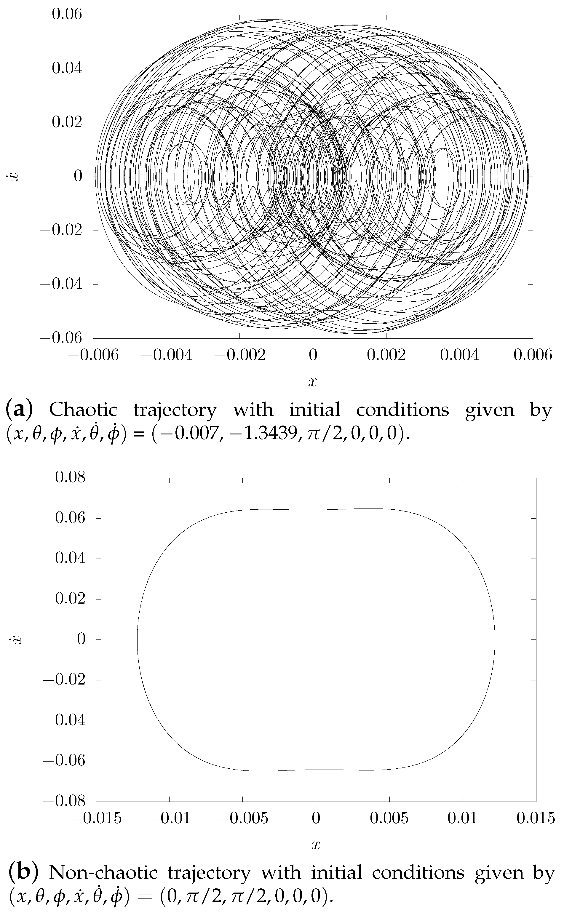
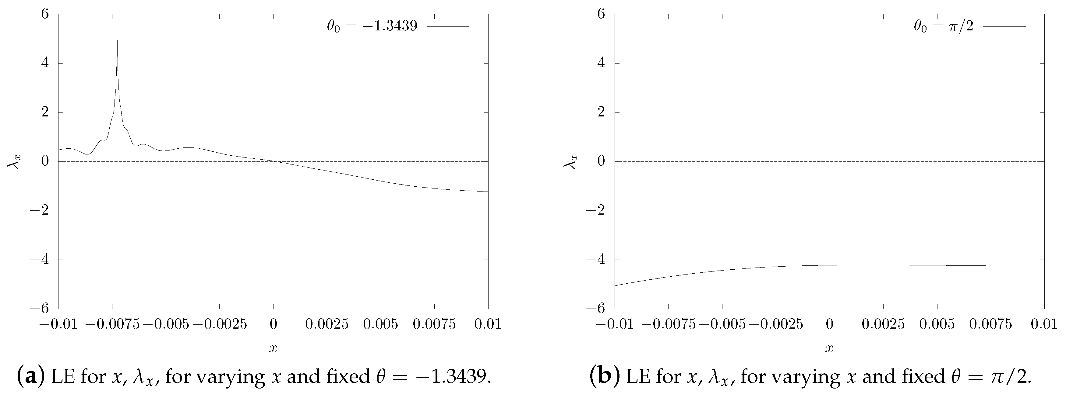
4. Physical Experiments

The system has six degrees of freedom, two of which were varied simultaneously. The initial conditions that remained fixed in each simulation of the dynamical system were: ${\varphi }_0=\pi /2$ and ${\dot{x}}_0={\dot{\theta }}_0={\dot{\varphi }}_0=0.0$. The initial conditions that were simultaneously swept were: $\left|x_0\right|\le 0.01$ and $\left|\theta \right|\le \pi /2$, with $dx=0.0001$ and $d\theta =\pi /180$, giving a total of 200 iterations in x and 180 iterations in $\theta$. It ought to be noted that the scanning regions are imposed by the physical limitations of the model. In this way, the sweeping of both initial conditions constitutes a total of $36,000$ Runge–Kutta instances to execute, each one simulated for 600 s (10 min) with $\Delta t=0.0001$ ($6\times {10}^7$ iterations).

For this experiment, the parameters of the model were initialised as follows: $A=0.0055555$ m, $k=5.15$ N/m, $\omega =2\pi$ Hz, $g=9.78$ kg s${}^{-2}$ (this value of gravity’s acceleration is valid in Mexico City, where the experiments were performed), $m_g=0.0686$ kg, $m_{\theta }=m_{\varphi }=0.0049$ kg, $l_{\theta }=l_{\varphi }=0.22$ m and $\gamma =0.029$ kg s${}^{-1}$.

The system does exhibit both chaotic and stable regions for the time span herein studied. There are three characteristic times in this system: $t_{c_x}=2\pi /\omega =1$ s and $t_{c_{\theta }}=t_{c_{\varphi }}\approx 1.11232$ s (when oscillating pendula are initially dropped from $\pi /2$). As an illustrative issue, we show phase planes for x, for chaotic and a non-chaotic cases, in Figure 1. The initial conditions for the chaotic trajectory are given by: $(x,\theta ,\varphi ,\dot{x},\dot{\theta },\dot{\varphi })=(-0.007,-1.3439,\pi /2,0,0,0)$. Meanwhile, for the non-chaotic trajectory the initial conditions were: $(x,\theta ,\varphi ,\dot{x},\dot{\theta },\dot{\varphi })=(0,\pi /2,\pi /2,0,0,0)$.

In Figure 2, Lyapunov exponents for varying x and fixed $\theta$ are shown. The chaotic phase plane trajectory shown in Figure 1a has a Lyapunov exponent, ${\lambda }_x=1.584224$, that corresponds to that of Figure 2a with $x=-0.007$. On the other hand, the non-chaotic phase plane trajectory shown in Figure 1b has a Lyapunov exponent, ${\lambda }_x=-4.214377$, as shown in Figure 2b with $x=0$

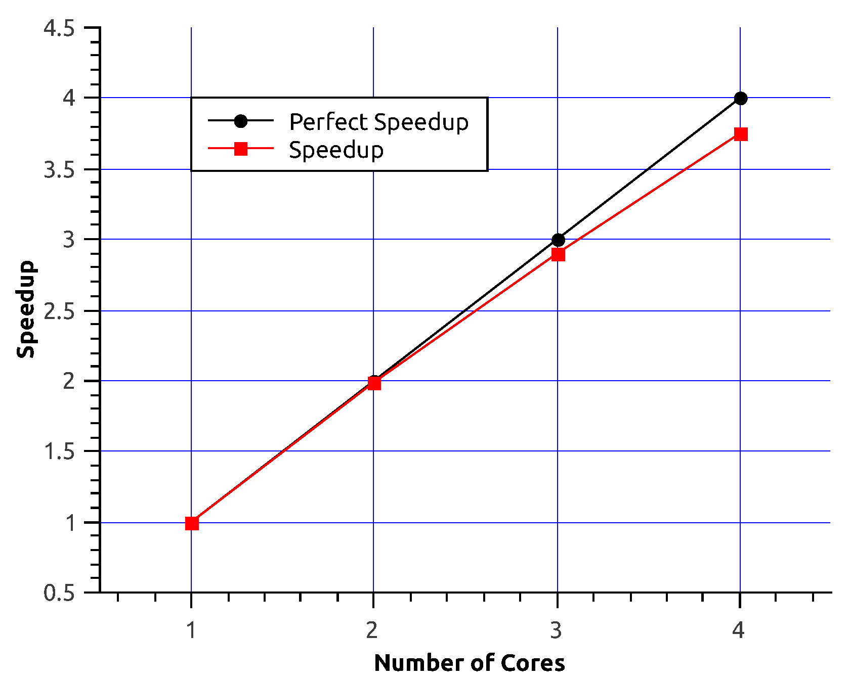
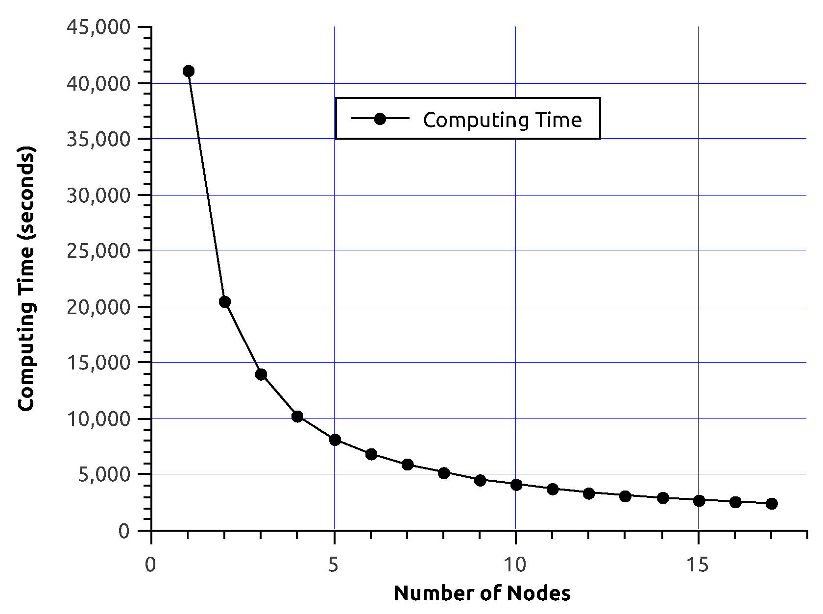
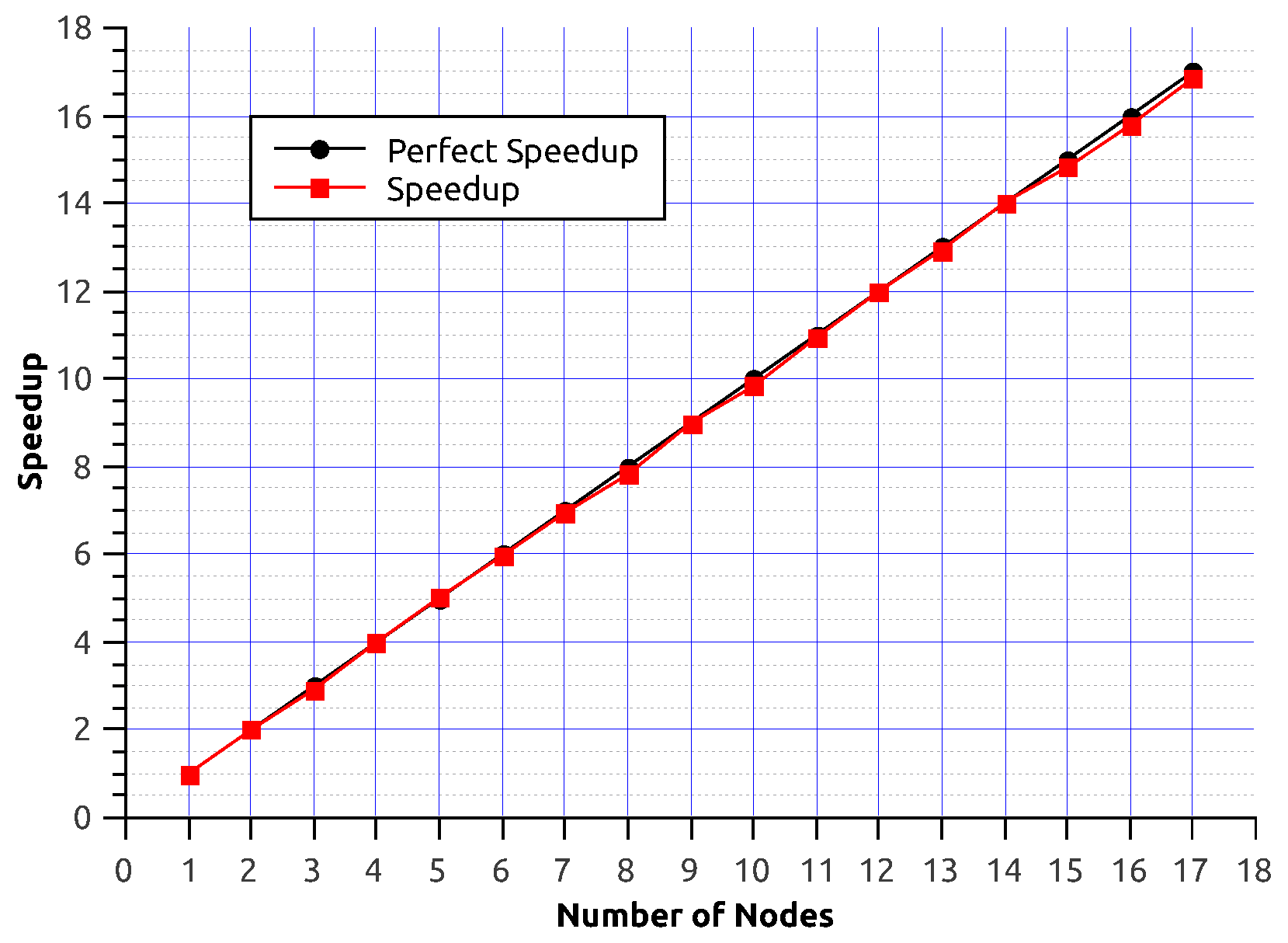
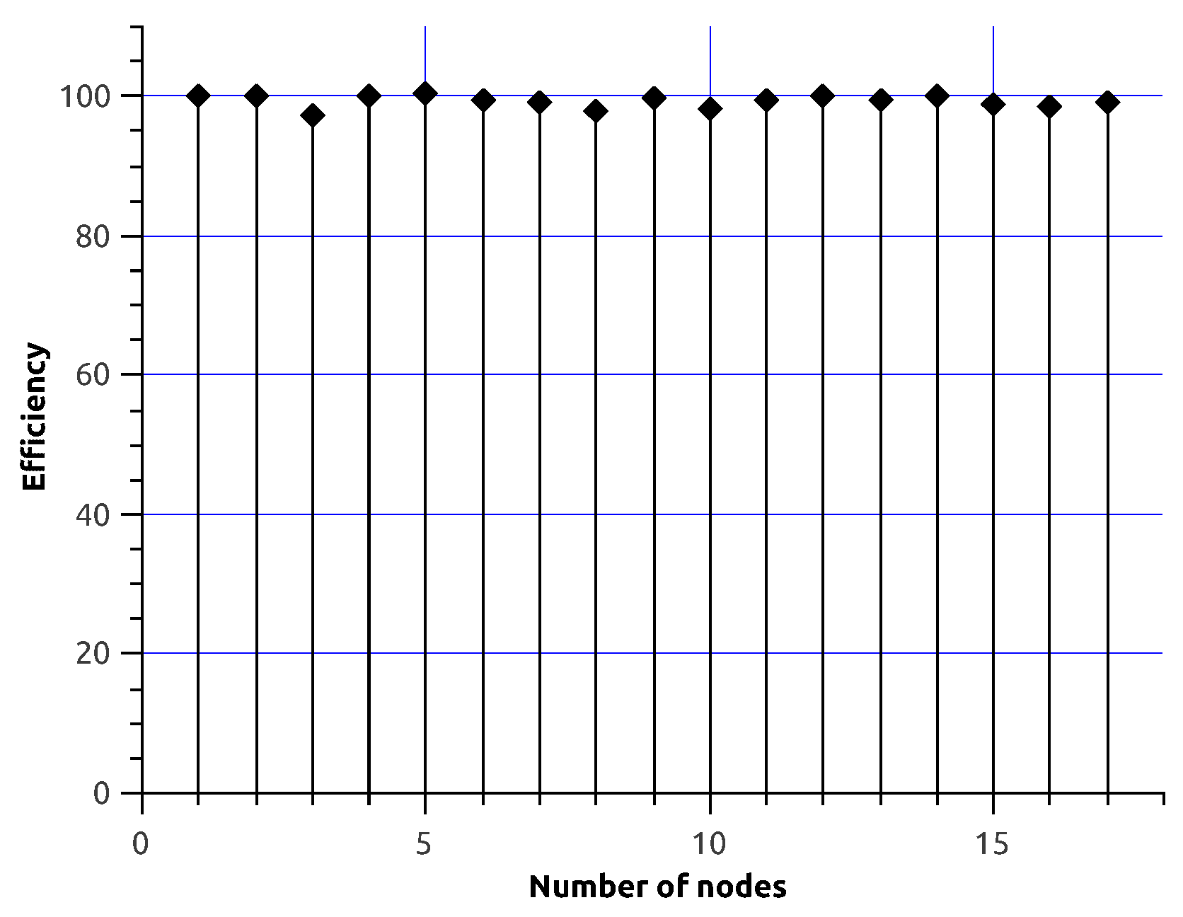
5. Performance Experiments

We started the experiments over a node to verify the performance without the latency of the network. We ought to recall the importance of controlling the affinity so that the MPI processes do not commute within the node and so that the final result remains as reliable as possible. Thus, the following environment variable was defined: export I_MPI_PIN_PROCESSOR_LIST=allcores:grain=core.

In Figure 3 we show the speed-up obtained using just one node with four cores executing from one to four MPI processes. The behaviour is practically linear, so the serial fraction is very low.

From Figure 3 we can conclude that execution time is considerably reduced. In the next experiment we launch from 1 to 17 MPI processes to measure, taking one node as a unit of computation, the performance. In Figure 4 we show computing times per computation unit, while in Figure 5 we feature the corresponding speed-up along the cluster. From the results we can observe a low introduction of the overhead latency as expected in the design.

An important metric indicator which must be calculated is the efficiency E, defined as

$$E=\frac{S\left(n\right)}{n}\times 100\%$$

(18)

where $S\left(n\right)$ is the obtained speed-up with n processes, and indicates how busy are the nodes during execution. Figure 6 shows that the efficiency obtained is high, since on average every node is kept busy 99.3% of the time. The efficiency also indicates that the partitioning of tasks herein implemented is scalable, which means that we can increase the number of computing units to improve time reduction while not losing efficiency in the use of many nodes. The scalability must be contemplated as a good design of the parallel program, since it allows scaling of the algorithm, a fact that we could expect when increasing the number of processing units in the cluster. Similar implementations where the problem consists of processing recursively the first, second, third, and fourth Runge–Kutta coefficients in a parallel fashion, achieve a maximum performance which decreases when adding more processing units [19].

6. Conclusions

A parallel design for the calculation of Lyapunov exponents in non-linear dynamical systems field was implemented and validated using MPI implementation. The numerical experiments and the obtained indicators validate the high efficiency of the implementation herein proposed, being able to overcome the networking speed.

As is well known, it is necessary to use the most convenient implementation that contributes to the attainment of the best performance or the greatest exploitation of the platform. For our case, distributing the calculation of serial Runge–Kutta problems is more efficient than using a parallelised version of the ODE solving method. Moreover, not only with respect to the performance we obtain excellent speed-ups, but this scheme results in an easier implementation of the parallelisation.

Finally, we must say that the parallelisation of the calculation of Lyapunov exponents, in the field of non-linear dynamical systems, allows researchers to drastically reduce the required time for exhaustive exploration of the manifold of initial conditions in order to quickly and accurately identify chaotic and non-chaotic dynamical regions, discarding, through high-latency and low-cost clusters, regions that appear to be chaotic that arise from large-sized temporal or spatial steps.

References

1. Strogatz, S. Nonlinear Dynamics and Chaos: With Applications to Physics, Biology, Chemistry, and Engineering; Studies in Nonlinearity; Avalon Publishing: New York, NY, USA, 2014. [Google Scholar]
2. Lyapunov, A.M. The General Problem of the Stability of Motion. Ph.D. Thesis, University of Kharkov, Kharkiv Oblast, Ukraine, 1892. [Google Scholar]
3. Benettin, G.; Galgani, L.; Strelcyn, J.M. Kolmogorov entropy and numerical experiments. Phys. Rev. A 1976, 14, 2338. [Google Scholar] [CrossRef]
4. Contopoulos, G.; Galgani, L.; Giorgilli, A. On the number of isolating integrals in Hamiltonian systems. Phys. Rev. A 1978, 18, 1183. [Google Scholar] [CrossRef]
5. Sato, S.; Sano, M.; Sawada, Y. Practical methods of measuring the generalized dimension and the largest Lyapunov exponent in high dimensional chaotic systems. Prog. Theor. Phys. 1987, 77, 1–5. [Google Scholar] [CrossRef]
6. Kantz, H. A robust method to estimate the maximal Lyapunov exponent of a time series. Phys. Lett. A 1994, 185, 77–87. [Google Scholar] [CrossRef]
7. Kuznetsov, N.; Alexeeva, T.; Leonov, G. Invariance of Lyapunov exponents and Lyapunov dimension for regular and irregular linearizations. Nonlinear Dyn. 2016, 85, 195–201. [Google Scholar] [CrossRef]
8. Wolf, A.; Swift, J.B.; Swinney, H.L.; Vastano, J.A. Determining Lyapunov exponents from a time series. Phys. D Nonlinear Phenom. 1985, 16, 285–317. [Google Scholar] [CrossRef]
9. Hernández-Gómez, J.J.; Couder-Castañeda, C.; Gómez-Cruz, E.; Solis-Santomé, A.; Ortiz-Alemán, J.C. A simple experimental setup to approach chaos theory. Eur. J. Phys. 2017. under review. [Google Scholar]
10. Rauber, T.; Rünger, G. Parallel Programming: For Multicore and Cluster Systems; Springer Science & Business Media: New York, NY, USA, 2013; pp. 1–516. [Google Scholar]
11. Couder-Castañeda, C. Simulation of supersonic flow in an ejector diffuser using the JPVM. J. Appl. Math. 2009, 2009, 497013. [Google Scholar] [CrossRef]
12. Kshemkalyani, A.; Singhal, M. Distributed Computing: Principles, Algorithms, and Systems; Cambridge University Press: Cambridge, UK, 2008; pp. 1–736. [Google Scholar]
13. Iserles, A.; Nørsett, S. On the Theory of Parallel Runge—Kutta Methods. IMA J. Numer. Anal. 1990, 10, 463. [Google Scholar] [CrossRef]
14. Bylina, B.; Potiopa, J. Explicit Fourth-Order Runge–Kutta Method on Intel Xeon Phi Coprocessor. Int. J. Parallel Program. 2017, 45, 1073–1090. [Google Scholar] [CrossRef]
15. Murray, L. GPU Acceleration of Runge-Kutta Integrators. IEEE Trans. Parallel Distrib. Syst. 2012, 23, 94–101. [Google Scholar] [CrossRef]
16. Majid, Z.; Mehrkanoon, S.; Othman, K. Parallel block method for solving large systems of ODEs using MPI. In Proceedings of the 4th International Conference on Applied Mathematics, Simulation, Modelling—Proceedings, Corfu Island, Greece, 22-25 July 2010; pp. 34–38. [Google Scholar]
17. Couder-Castañeda, C.; Ortiz-Alemán, J.; Orozco-del Castillo, M.; Nava-Flores, M. Forward modeling of gravitational fields on hybrid multi-threaded cluster. Geofis. Int. 2015, 54, 31–48. [Google Scholar] [CrossRef]
18. Arroyo, M.; Couder-Castañeda, C.; Trujillo-Alcantara, A.; Herrera-Diaz, I.E.; Vera-Chavez, N. A performance study of a dual Xeon-Phi cluster for the forward modelling of gravitational fields. Sci. Program. 2015, 2015, 316012. [Google Scholar] [CrossRef]
19. Zemlyanaya, E.; Bashashin, M.; Rahmonov, I.; Shukrinov, Y.; Atanasova, P.; Volokhova, A. Model of stacked long Josephson junctions: Parallel algorithm and numerical results in case of weak coupling. In Proceedings of the 8th International Conference for Promoting the Application of Mathematics in Technical and Natural Sciences—AMiTaNS 16, Albena, Bulgaria, 22–27 June 2016; Volume 1773. [Google Scholar]
Figure 1. Phase plane trajectories of x showing long-term chaotic (a) and non-chaotic (b) behaviour. (a) corresponds to λ x = 1.584224 as shown in Figure 2a, while (b) corresponds to λ x = 4.214377 as shown in Figure 2b.
Algorithms 10 00137 g001
Figure 2. Lyapunov exponents for varying x and fixed θ . (a) shows two regions. The first half describes chaos, while the second half shows stability. (b) has a large region of pure stability.
Algorithms 10 00137 g002
Figure 3. Speed-up obtained in one node. As can be observed the speed-up is almost linear. The computing times are 154,158 s, 77,395 s, 53,214 s and 41,082 s.
Algorithms 10 00137 g003
Figure 4. Computing times obtained from 1 to 17 processes in the cluster; the processes follow an ordered affinity.
Algorithms 10 00137 g004
Figure 5. Speed-up obtained in the cluster. The perfect speedup is 17 and the obtained speedup is 16.85, giving us a very good performance.
Algorithms 10 00137 g005
Figure 6. Efficiency on the cluster.
Algorithms 10 00137 g006