A Hierarchical Multi-Label Classification Algorithm for Gene Function Prediction

Abstract

Gene function prediction is a complicated and challenging hierarchical multi-label classification (HMC) task, in which genes may have many functions at the same time and these functions are organized in a hierarchy. This paper proposed a novel HMC algorithm for solving this problem based on the Gene Ontology (GO), the hierarchy of which is a directed acyclic graph (DAG) and is more difficult to tackle. In the proposed algorithm, the HMC task is firstly changed into a set of binary classification tasks. Then, two measures are implemented in the algorithm to enhance the HMC performance by considering the hierarchy structure during the learning procedures. Firstly, negative instances selecting policy associated with the SMOTE approach are proposed to alleviate the imbalanced data set problem. Secondly, a nodes interaction method is introduced to combine the results of binary classifiers. It can guarantee that the predictions are consistent with the hierarchy constraint. The experiments on eight benchmark yeast data sets annotated by the Gene Ontology show the promising performance of the proposed algorithm compared with other state-of-the-art algorithms.

1. Introduction

In recent years, the diverse applications of hierarchical multi-label classification (HMC) are studied in several domains, such as text categorization, digital libraries, and gene function prediction [1]. In these real world problems, each instance may have many classes simultaneously. These classes are organised in a predefined hierarchical structure [2], and an instance associated with one class is automatically assigned with all its ancestor classes [3]. Gene function prediction is a complicated HMC problem, as a single gene may have many functions and these functions are structured according to a predefined hierarchy [4]. A directed acyclic graph (DAG) for the Gene Ontology (GO) and a rooted tree for the Functional Catalogue (FunCat) are two main hierarchy structures of gene functional classes [5]. The former one is more complicated to cope with, due to the fact that a node in a DAG can have many parent nodes [6], so the classification on the GO taxonomy of DAG structure is our focus in this paper.

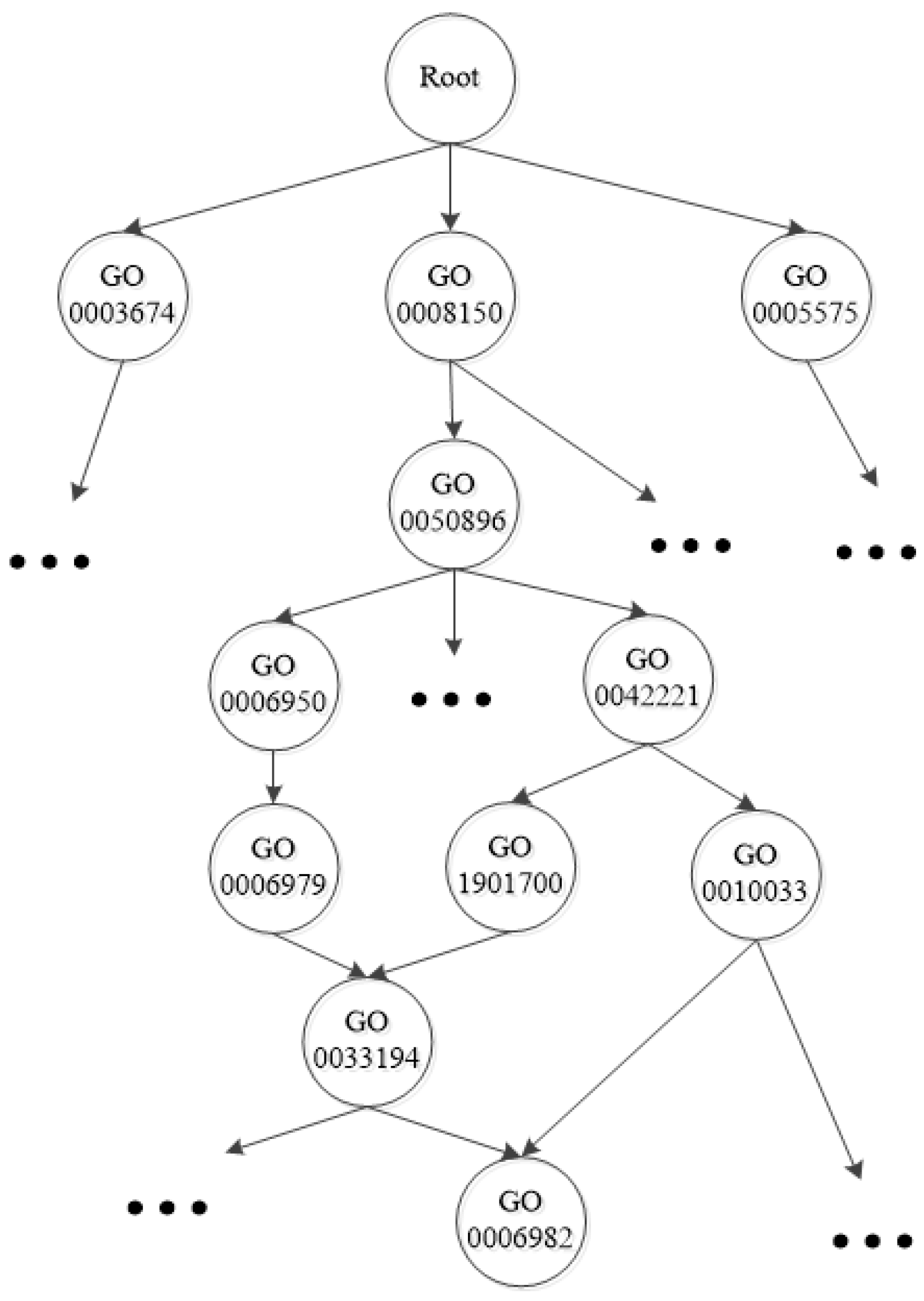
The Gene Ontology [7] is a widely used protein function classification scheme. It is made up of thousands of functional class terms and each term corresponds to a functional class.The hierarchy structure of the GO is a DAG. The GO contains three separated parts: biological process ontology, molecular function ontology and cellular component ontology [8]. Each of them is also organized as a DAG. Figure 1 illustrates a fraction of the Gene Ontology taxonomy.

Some classification algorithms have been designed to solve the HMC tasks, and these algorithms could be divided into two types: the global approach and the local approach [9].

Only a single model is generated in the global approach, and it predicts all the labels of an instance during a single run of the classification model [10]. When the size of the data set increases, the model usually becomes very complex and thus time-consuming [11]. The algorithms proposed in paper [12,13] are examples of the global approach.

The local approach transforms a HMC task into a separate binary classification task for each class, and then combines the results of all binary classifiers by considering the hierarchy [14]. It is easy to solve the complicated HMC problems with high dimensional attributes by using conventional classification algorithms [15]. Barutcuoglu et al. [16] selected support vector machine (SVM) as the base classifier for every class in the method they proposed. The results of these base classifiers were processed via a Bayesian network to guarantee the hierarchy constraint for the final results. Valentini et al. [17] presented a true path rule (TPR) hierarchical ensemble method to deal with the tree structure by using probabilistic SVMs for binary classifications. Chen et al. [15] improved the TPR approach for the tree structure. Robinson et al. [18] proposed a TPR ensemble strategy for the DAG structure.

There are two major challenges when applying the local approach to tackle the HMC task using the GO taxonomy. Firstly, as the hierarchy is traversed down to the leaves, classes at lower levels of the hierarchy usually have very fewer positive instances, requiring base classifiers at these hierarchy levels to be learned from very skewed data sets [19]. In such imbalanced data set learning scenarios, standard classifiers might be overwhelmed by the majority class and can not detect the minority one. Secondly, the prediction result needs to be consistent with the hierarchy constraint. It means an instance should automatically belong to all the ancestor classes of the class to which it belongs, and an instance should not belong to any of the descendant classes of the class to which it does not belong [20].

Conventional HMC methods in published papers mainly focus on these challenges for the FunCat taxonomy because the structure of it is easy to tackle. These days, the Gene Ontology has become the most popular functional classification scheme for gene and protein function prediction studies [21], but only a few HMC methods have been proposed for the GO as its DAG structure is more complicated to handle. In this paper, we deal with these problems based on the GO taxonomy.

For the gene function prediction problem based on GO, a hierarchical multi-label classification algorithm is proposed in this paper. Specifically, we make the following contributions. Negative instances selecting policy and a synthetic minority over-sampling technique (SMOTE) [22] are introduced to preprocess the imbalanced training data sets; in the proposed algorithm, SVM is chosen as the base classifier considering its good performance for binary classification; a two-phase approach based on the Bayesian network is used for combining the outputs of all binary classifiers to guarantee the hierarchy constraint. All of these techniques together lead to the improvement of the final gene function prediction results. Experiments are implemented to evaluate the performance of the proposed algorithm on eight benchmark data sets by comparing it with state-of-the-art algorithms. The experimental results indicate that the algorithm has better performance than the existing algorithms.

The rest of this paper is organized as follows. Section 2 revisits the definition of hierarchical multi-label classification and shows the proposed HMC algorithm for the GO. Experimental results on the eight benchmark GO data sets are given in Section 3. The discussion is presented and then, in the last section, the conclusions are introduced.

2. The Proposed Algorithm

2.1. Notation and Basic Definitions

Let X be a set of n gene instances, $x_i$ be any gene instance with m attributes written as $x_i=(a_1,a_2,\dots ,a_m),$ where $x_i\in X$$(1\le i\le n)$. Let C be a set of all the GO classes, $C=\{c_1,c_2,\dots ,c_{|C|}\}$. The GO hierarchy is a DAG denoted by $G=<V,E>$. $V=\{1,2,\dots ,|V|\}$ is the set of vertices and the edges set is E, where $e=(k,l)\in E,k,l\in V$ means an edge. Each node in V represents a class, so $V=C$ and the class $c_k$ is represented simply by the node k if there is no ambiguity. Each node represents one gene function, and a direct edge $e=(k,l)\in E$ describes the hierarchical relationship that k is the parent node of l. We further denote the set of children nodes of a node k as $child(k)$, the set of its parent nodes as $par(k)$, the set of its ancestor nodes as $anc(k)$, the set of its descendant nodes as $desc(k)$ and the set of its siblings as $sib(k)$.

Given an instance $x_i\in X$, if $x_i$ has the function the node k presents, the real label at the node k is 1, and this is also called that this instance $x_i$ belongs to the node k. If there is no ambiguity, it is said that its node k is 1 for short. The result of a binary classifier $f_k$ for the class $c_k$ is denoted as $d_{ik}^{*}$, where $1\le k\le |C|$, and it is used to predict the label of $x_i$ at node k. $d_{ik}^{*}$ represents the probability of the instance $x_i$ belonging to the node k given by this classifier $f_k$, which is also written as $P_i^{*}(k=1)$.

The set of $|C|$ binary classifiers provides a multi-label score $d_i^{*}=(d_{i1}^{*},d_{i2}^{*},\dots ,d_{i|C|}^{*})$, which is called the preliminary results. The preliminary predicted label for an instance $x_i\in X$ with all the classes is denoted as a vector $y_i^{*}=(y_{i1}^{*},y_{i2}^{*},\dots ,y_{i|C|}^{*})$ for $1\le k\le |C|$. It is obtained by selecting a threshold $\theta$ for $d_i^{*}$. If $d_{ik}^{*}\ge \theta$, set $y_{ik}^{*}=1$, the representing $x_i$ belongs to class $c_k$; otherwise, set $y_{ik}^{*}=0$ for $1\le k\le |C|$. We say that this result for an instance $x_i$ is consistent with the hierarchy constraint if and only if $d_{ik}^{*}\ge d_{il}^{*}$, where k is the parent class of l. The final predicted score at the node k is written as $d_{ik}$, which is the posterior probability $P_i(k=1)$. If we get the consistent preliminary result, then $d_i=d_i^{*}$; otherwise, we need to use other methods to get the final consistent score $d_i$. Similarly, the final prediction vector $y_i=(y_{i1},y_{i2},\dots ,y_{i|C|})$ can be obtained by selecting a threshold $\theta$ for $d_i$.

2.2. The Main Steps of the Proposed Method

The proposed algorithm contains four steps. Its main processes are described as follows. The first step is the data set preparing step. In this step, training data set is partitioned into $|C|$ subsets by utilizing negative instances selecting policy, where $|C|$ means the total number of all the classes in the GO. The second step is the data set rebalancing step, where the over-sampling technique is applied to modify the data distribution. Then, $|C|$ binary classifiers, which are also called base classifiers or local classifiers, are trained by using these training subsets in the third step. The final step is the prediction step. In the prediction phase, the instances in the test set are first predicted by $|C|$ binary classifiers; then, these results are changed into probabilities by the sigmoid method. Finally, these probabilistic prediction results are combined by the nodes interaction method to ensure the hierarchy constraint.

2.3. Step 1: Training Data Set Preparation

Selecting suitable positive and negative instances to build the training set is very important for a classifier. To explore the hierarchical structure, according to the paper [23], the siblings policy is suggested for building the training subset for each class, which is designed as follows. For the training data set of the class k, instances that belong to k are chosen as the positive instances, and other instances belonging to the siblings of k are selected as negative instances. In the case that the class k has no siblings, instances that belong to the siblings of its parent nodes are selected [24].

2.4. Step 2: Data Set Rebalancing

In the HMC problems, from the top to the bottom of the hierarchy, as the specificity of the classes increases, fewer number of instances are annotated to more specific classes, so there are many more instances of some classes than others. As the hierarchy level lowers, the number of instances belonging to the class drops significantly. Most of the binary classifiers need to be learned from strongly skewed training data sets. Such case is called an imbalanced data set, which leads to difficulty in making accurate predictions for standard classifiers, since the minority class tends to be overwhelmed by the majority one [25]. In step 1, a negative instances selecting policy is proposed to alleviate the imbalanced data set problem.

Even after using the siblings policy to build training subsets for all classes, the training subsets of some classes are still high degree imbalanced. In order to change the distribution of the training data set, re-sampling method is used to augment either some positive instances or some negative instances.

SMOTE proposed in [22] is an efficient re-sampling approach. It produces new synthetic instances along the line between the minority instances and their selected nearest neighbor instances. The advantage of this method is that it changes the decision domains to be larger and less specific. SMOTE creates synthetic minority instances to over-sample the minority class. For each minority instance, a certain number (it is usually set to 5 as a default) of its nearest neighbor instances at the same class are figured out first; then, some instances are randomly chosen from them according to the over-sampling rate. After this step, new synthetic instances are produced.

In the GO hierarchy, the classes at higher levels may have more positive instances than negative ones, and, therefore, the negative class is the minority class. On the contrary, for the lower classes, there are more negative instances, and the positive class is the minority class. SMOTE is used to over-simplify the minority instances for each training subset. Then, a balanced data set is provided to the binary classifier to enhance the detection rate of the minority class.

2.5. Step 3: Base Classifier Training

After the two steps above, we build a particular data set per node, and get $|C|$ different balanced data sets for $|C|$ classes totally. For each node, an SVM is trained by using the training data set at this node. The reason for choosing SVM as the base classifier is that it performs best among the state-of-the-art classifiers, and its good ability to tackle the classification problems that are linearly inseparable [26].

The result of SVM should be changed into the probability, which is needed by the nodes interaction method. As the standard SVM does not give such probability, the sigmoid method is often used to figure out the probabilistic result of SVM [27]. It changes the output of the SVM to probability by training an additional sigmoid function, which is described as follows:

$$ps(y=1|x)=\frac{1}{1+exp(Af(x)+B)},$$

(1)

where x is an instance, y represents the class label of x, $f(x)$ is the output of SVM for x, and A and B are the parameters. To calculate these two parameters A and B, any validated subset with $n^{\prime }$ instances of the training data set could be applied to solve the following maximum likelihood problem, where $i=1,2,\dots ,n^{\prime }$:

$$\underset{Z=(A,B)}{min}\{-\sum _{i=1}^l(t_{i}log(p{s}_i)+(1-t_i)log(1-p{s}_i))\},$$

(2)

$$p{s}_i=\frac{1}{1+exp(Af(x_i)+B)},$$

(3)

$$t_i=\left\{\begin{array}{c}\frac{N_{+}+1}{N_{+}+2}{y}_i=1,\hfill \\ \frac{1}{N_{-}+2}{y}_i=-1.\hfill \end{array}\right.$$

(4)

2.6. Step 4: Prediction

In this step, the instances that need to be predicted are first classified by $|C|$ base classifiers and get the probabilistic preliminary results. As the base classifiers are trained separately, these preliminary results usually violate the TPR rule, so we need some method to ensure that the final results are consistent with the hierarchy constraint. The TPR rule is also described as the hierarchy constraint, which guarantees the consistency of the function annotations in the GO [28].

In practice, for a given instance $x_i$, considering a node k, $d_{ik}^{*}$ is the preliminary result calculated by the binary classifier at this node, if $y_{ik}^{*}$ shows that $x_i$ has the label 0 at this node k, but some preliminary results of its children nodes $d_{ichild(k)}^{*}$ are 1; in this case, the preliminary results for the given instance $x_i$ violate the TPR rule. When such case occurs, we need to use some methods to revise the results of $x_i$ to ensure the final results obey the TPR rule. In this paper, a novel method based on the Bayesian network is proposed to tackle this problem [29], which is called the nodes interaction method.

The nodes interaction method is designed to resolve the problem that the results of parent and children nodes are inconsistent with the hierarchy. The key idea of this method is that, when determining the final predicted labels, the hierarchy of the classes should be considered. As the GO hierarchy is a DAG structure, the prediction of a node is not only decided by its base classifier, but also influenced by its adjacent nodes, such as parent or children nodes.

There are two phases in the nodes interaction method: preliminary results correction phase and final decision determination phase. In the preliminary results correction phase, for each instance, the DAG is visited from top to bottom across the hierarchy to correct the predictions that violate the TPR rule. The main purpose of this step is to consider the influence of its parent and children nodes when making decisions for a node.

As the base classifier of each node provides the probability for which label an instance should have at this node, this preliminary result can be seen as prior probability of this instance at this node. These nodes are organized as a DAG, and we want to get the final result of an instance at each node, which is to calculate the posterior probability of this instance at each node. This circumstance is very similar to the Bayesian network [30]. Given an instance $x_i$, its preliminary result at node k is $d_{ik}^{*}$, and $d_{ik}^{*}$ along with the results at parent nodes $d_{ipar(k)}^{*}$ or at children nodes $d_{ichild(k)}^{*}$ violate the true path rule. In the preliminary results’ correction phase, the Bayesian network is used to make the decision at the node k.

For the instance $x_i$, considering the node k, its parent nodes $par(k)$ and children nodes $child(k)$, the DAG is detached into two parts: the parent nodes part and the children nodes part. The Bayesian network is utilized in each part, respectively, to calculate the posterior probability $P(k=1)$. When only considering the parent nodes of a particular node k, the posterior probability $P(k=1)$ is denoted as $P_{par}(k)$, and the formula to get $P_{par}(k)$ is:

$$\left\{\begin{array}{c}{P}_{par}(k=1)=P^{*}(k=1)\prod _{j\in par(i)}{P}^{*}(j=1),\hfill \\ P_{par}(k=0)=1-P_{par}(k=1).\hfill \end{array}\right.$$

(5)

Similarly, when considering the children nodes of a particular node k, the formula of $P_{child}(k)$ is:

$$\left\{\begin{array}{c}{P}_{child}(k=0)=P^{*}(k=0)\prod _{j\in par(i)}{P}^{*}(j=0),\hfill \\ P_{child}(k=1)=1-P_{child}(k=0).\hfill \end{array}\right.$$

(6)

To make the final decision, we compare these two probabilities $P_{par}(k=0)$ and $P_{child}(k=1)$, and select the bigger one as the decision of this phase. More precisely, for a node k, let ${\widehat{y}}_k=p{s}_k$, and ${\tilde{y}}_k$ be the result of x to be calculated in the preliminary results correction phase. It is derived as follows:

$${\tilde{y}}_k=\left\{\begin{array}{cc}{P}_{par}(k=1),\hfill & if{P}_{par}(k=0)\ge P_{child}(k=1),\hfill \\ P_{child}(k=1),\hfill & otherwise.\hfill \end{array}\right.$$

(7)

The main goal of the preliminary results correction phase is to consider the influence of its parent and children nodes when making decision for a node, but it cannot ensure the hierarchical consistent of the predictions. The final decision determination phase is introduced to assure the hierarchical consistent of the predictions by propagating negative decisions towards the children nodes recursively. It modifies the results computed in the previous phase by visiting all the nodes again from top to bottom of the DAG. If ${\tilde{y}}_k$ is the prediction computed in the first phase, then the final predictions ${\overline{y}}_k$ for the class k are calculated as follows:

$${\overline{y}}_k=\left\{\begin{array}{cc}{\tilde{y}}_k,\hfill & ifkisarootnode,\hfill \\ \underset{j\in par(k)}{min}{\overline{y}}_j,\hfill & if{\tilde{y}}_k>\underset{j\in par(k)}{min}{\overline{y}}_j,\hfill \\ {\tilde{y}}_k,\hfill & otherwise.\hfill \end{array}\right.$$

(8)

3. Experiment

3.1. Data Sets and Experimental Setup

Several real-world databases from the field of functional genomics downloaded from the DTAI website refer to paper [13] were selected to evaluate the proposed algorithm [31]. Since Saccharomyces cerevisiae, which is a type of baker’s or brewer’s yeast, is one of the well-studied model organisms with high-throughput data available, the task is to predict gene functions of the yeast. In this paper, we worked with eight data sets annotated by the GO structured as a DAG. Each data set describes a different aspect of the genes in the yeast genome. For example, the data set 8 (seq) contains the sequence statistics data of each gene, which include the sequence length, molecular weight and so on. The detailed description of these yeast data sets can be obtained to from paper [13].

The characteristics of the experimental data sets, such as instance number and attribute number of each data set, are summarized in

Table 1. The characteristics of the experimental datasets.

Data Set	Attributes	Training Instances	Testing Instances
D1 Cellcycle	77	2290	1202
D2 eisen	79	2252	1182
D3 derisi	63	1537	817
D4 gasch1	173	2294	1205
D5 gasch2	52	1301	1212
D6 church	27	2289	1202
D7 spo	80	2354	1183
D8 seq	478	2321	1225

.

As in [13], two thirds of each data set is used as the training data set and the remaining one third for testing. In each training set, two thirds of it is used for the actual training and the remaining one third is for optimizing parameters. In addition, as some of the data sets contain missing features, the mean of the non-missing values for that feature have managed to replace the missing values of that feature [32].

We downloaded the GO file from the GO website [21], which includes hierarchical relationships between different GO terms [33]. The Gene Ontology Annotation (GOA) file of Yeast was obtained from the European Bioinformatics Institute. The GO terms annotated as ‘obsolete’ were excluded from the GO file. The GOA file was processed to only include the annotations with evidence codes EXP (Inferred from Experiment), IDA (Inferred from Direct Assay), IPI (Inferred from Physical Interaction), IMP (Inferred from Mutant Phenotype), IGI (Inferred from Genetic Interaction), IEP (Inferred from Expression Pattern), TAS (Traceable Author Statement ) or IC (Inferred by Curator) [34]. Among three separated ontology in the GO, we focus on the biological process aspect for the experiment in this study.

Assuming that rare classes cannot be reliably induced, only the nodes with more than 100 instances are considered. The resultant DAG has a depth of 11, and each instance has labels, on average, of 32. The threshold of each binary classifier SVM is set as 0.5 in all experiments.

3.2. Evaluation Metrics

Due to the hierarchy and multi-label pecularities of the HMC problem, two sorts of metrics are used to evaluate the proposed algorithm. The first metric category is the classical precision ($Prec$), recall ($Rec$), and $F_1$ [35]. These metrics are mainly designed for the binary classification task with only two classes. We don’t select the accuracy ($Acc$) as the evaluation metric because it is not suitable for the imbalanced data set problem. Precision expresses the ratio of positive predictions that are labelled correctly, and recall is the percentage of positive instances that are exactly predicted as positive. $F_1$ is a parameter to combine the tradeoff of $Prec$ and $Rec$ in a single formula. These three metrics are used to evaluate the binary base classifiers:

$$Prec=\frac{TP}{TP+FP},$$

(9)

$$Rec=\frac{TP}{TP+FN},$$

(10)

$$F_1=\frac{2\times Prec\times Rec}{Prec+Rec},$$

(11)

where $TP$ is the number of true positives (positive instances that are correctly predicted as positive), $FP$ is the number of false positives (negative predictions that are incorrectly predicted as positive), and $FN$ is the number of false negatives (positive instances that are incorrectly predicted as negative). Note that these measures do not take into account the number of the negative instances that are predicted correctly.

How to evaluate the performance of hierarchical classification algorithms is an open question. Some researchers used the above-defined classical metrics as evaluation measures, but these metrics might not show enough information about which algorithm is really better by not considering the structure of the hierarchy taxonomy [36]. Some authors proposed their own evaluation measures for hierarchical classification, but these measures are used by themselves only. Some evaluation measures such as h-loss are proposed for the tree-structured problems but can not cope with DAGs. Although at present, for all possible hierarchical classification tasks and applications, no hierarchical classification measure can be regarded as the best one, a set of relational metrics is proposed and suggested in [23] to use for evaluation. They are hierarchical precision, hierarchical recall and hierarchical $F_1$, which are denoted as $hPre$, $hRec$ and $h{F}_1$. These metrics are used widely by researchers.

The hierarchical precision, hierarchical recall and hierarchical $F_1$ for the i-th example $hPr{e}_i$, $hRe{c}_i$ and $h{F}_{1,i}$ are defined as :

$$hPr{e}_i=\frac{|\widehat{P_i}\bigcap \widehat{T_i}|}{|\widehat{P_i}|},$$

(12)

$$hRe{c}_i=\frac{|\widehat{P_i}\bigcap \widehat{T_i}|}{|\widehat{T_i}|},$$

(13)

$$h{F}_{1,i}=\frac{2\times hPr{e}_i\times hRe{c}_i}{hPre+hRec},$$

(14)

where, for a test instance i, $\widehat{P_i}$ is the set containing all of the predicted classes and their ancestor classes, and $\widehat{T_i}$ is the set including all of its true classes and their ancestor classes.

These measures are extended versions of the widely used metrics of precision, recall and $F_1$, and are specially designed for the hierarchical classification problem. Furthermore, they can be effectively adapted to both the tree and the DAG structures. Supposing the evaluation of the results measured on a data set with n instances labeled with m hierarchical structured classes, there are two methods to combine the performance of all instances: the micro-averaging version and the macro-averaging version [37].

In the micro-averaging version, the precision and recall are figured out by summing over all individual instances, and these metrics are given as follows:

$$hPr{e}^{\mu }=\frac{{\sum }_{i=1}^n|\widehat{P_i}\bigcap \widehat{T_i}|}{{\sum }_{i=1}^n|\widehat{P_i}|},$$

(15)

$$hRe{c}^{\mu }=\frac{{\sum }_{i=1}^n|\widehat{P_i}\bigcap \widehat{T_i}|}{{\sum }_{i=1}^n|\widehat{T_i}|},$$

(16)

$$h{F}_1^{\mu }=\frac{2\times hPr{e}^{\mu }\times hRe{c}^{\mu }}{hPr{e}^{\mu }+hRe{c}^{\mu }}.$$

(17)

In the macro-averaging version, the precision and recall are first computed for each instance and then averaged. The metrics are written as:

$$hPr{e}^M=\frac{{\sum }_{i=1}^{n}hPr{e}_i}{n},$$

(18)

$$hRe{c}^M=\frac{{\sum }_{i=1}^{n}hRe{c}_i}{n},$$

(19)

$$h{F}_1^M=\frac{{\sum }_{i=1}^{n}h{F}_{1,i}}{n}.$$

(20)

For all of these metrics, it should be noted that there is a common feature, the higher measure value means the better performance of a classifier. The hierarchical precision indicates the capability of a classifier to predict the most general functional classes of an instance, while the hierarchical recall shows the predictor’s ability to predict the most specific functional classes. The hierarchical F-measure takes into account both hierarchical precision and hierarchical recall to calculate an overall value [38].

3.3. Experiment Results and Analysis

3.3.1. Experiments for Specific Classes

To observe the performance of the data set rebalance method, which consists of the negative instances selecting policy and the SMOTE over-sampling method, we implemented binary experiments for specific classes. A comparative experiment is designed as follows: in step 1, when building training data set for each class, the positive instances are assigned according to the specified class, while the negative instances are all the others not labelled as positive in the data set. As in the comparative experiment, most of the training data sets are highly imbalanced, so the base classifier SVM tends to predict all test samples as negative, and these kinds of results show no significance. The D1 data set is used in this part to show the difference, and SVM is used as the base classifier. $Prec$, $Rec$ and $F_1$ are used for evaluation and part of the experimental results are shown in

Table 2. The experimental results for specific classes.

GO ID	Original $\mathit{Prec}$	Original $\mathit{Rec}$	Original ${\mathit{F}}_1$	Improved $\mathit{Prec}$	Improved $\mathit{Rec}$	Improved ${\mathit{F}}_1$
GO:0065007	NaN	0	NaN	0.408	0.454	0.430
GO:0016043	NaN	0	NaN	0.486	0.539	0.511
GO:0044710	0.577	0.121	0.206	0.478	0.433	0.455
GO:0006996	NaN	0	NaN	0.358	0.775	0.490
GO:0044249	0.552	0.181	0.272	0.440	0.630	0.518
GO:0046483	NaN	0	NaN	0.437	0.699	0.538
GO:1901360	0.750	0.013	0.025	0.448	0.734	0.557
GO:1901564	0.591	0.050	0.092	0.373	0.431	0.400
GO:0009059	0.472	0.045	0.082	0.384	0.451	0.415
GO:0019538	0.520	0.040	0.073	0.352	0.489	0.410
GO:0044271	0.500	0.011	0.021	0.344	0.603	0.438
GO:0034645	0.472	0.045	0.082	0.364	0.596	0.452

. “The original $F_1$” represents the results of the comparative data set and “the improved $F_1$” represents the results of the rebalanced data set, and NaN means that the result is not a number. The results show that the negative instances selecting policy associated with the SMOTE approach improved the performance of the base classifier.

3.3.2. Experiments on Eight Data Sets

This algorithm is designed to tackle the HMC problem for solving the gene function prediction task based on GO. To present the performance of this algorithm, it is also necessary to compare with other state-of-the-art algorithms. Due to the complexity of the HMC problem with DAG structure, only a few algorithms have been proposed by others. The TPR ensemble method and the CLUS-HMC method are two typical state-of-the-art algorithms used for gene function prediction. The TPR ensemble method is the representation of the algorithms that belongs to the local approach. It has better performance than other local algorithms such as the flat ensemble method and the hierarchical top-down method. As a representative of global algorithms, the CLUS-HMC method outperforms the HLCS-Multi algorithm, the HLCS-DAG algorithm and the HMC-LMLP algorithm. Thus, these two algorithms are selected to be compared with the proposed HMC algorithm. For consistency, we used the same data sets and the same evaluation scheme for each algorithm we tested. The details of these two methods are listed below.

The TPR ensemble method: this method integrates the predictions of base classifiers with the positive results that come from the classifiers at the lower level, together with the negative results that are given by the higher level classifiers [18]. The TPR ensemble method contains two steps. In the bottom-up step, the positive predictions are moved towards the parent nodes and gradually towards the ancestor nodes. In the top-down step, negative predictions are propagated to the children nodes and the descendant nodes of each node, aiming to ensure the consistency of the final results and also give more precise predictions [17].

CLUS-HMC [13]: this method belongs to the global approach, and it predicts all class labels at the same time by inducing a single decision tree. The predictive clustering tree framework is used in this algorithm. The hierarchy structure is considered by modifying different weights to the labels according to the level, and the DAG can also be solved by this method. The level parameter is selected through the cross validation, and the weighted Euclidean distances are designed for the variance reduction.

We computed both the micro-averaged version and macro-averaged version of $hPre$, $hRec$ and $h{F}_1$ to appraise the performance of the proposed algorithm. In

Table 3. The micro-averaged version of experimental results on eight data sets.

Dataset	Method	${\mathit{hPre}}^{\mathit{\mu }}$	${\mathit{hRec}}^{\mathit{\mu }}$	${\mathit{hF}}_1^{\mathit{\mu }}$
D1	TPR	0.348	0.518	0.416
D1	CLUS-HMC	0.449	0.306	0.364
D1	Proposed	0.333	0.627	0.435
D2	TPR	0.360	0.397	0.377
D2	CLUS-HMC	0.402	0.335	0.365
D2	Proposed	0.331	0.533	0.408
D3	TPR	0.434	0.515	0.471
D3	CLUS-HMC	0.476	0.387	0.427
D3	Proposed	0.396	0.663	0.496
D4	TPR	0.385	0.477	0.426
D4	CLUS-HMC	0.453	0.355	0.398
D4	Proposed	0.358	0.585	0.444
D5	TPR	0.359	0.519	0.425
D5	CLUS-HMC	0.442	0.322	0.373
D5	Proposed	0.333	0.623	0.434
D6	TPR	0.331	0.483	0.393
D6	CLUS-HMC	0.487	0.270	0.348
D6	Proposed	0.314	0.606	0.413
D7	TPR	0.366	0.423	0.393
D7	CLUS-HMC	0.418	0.331	0.369
D7	Proposed	0.339	0.541	0.417
D8	TPR	0.388	0.509	0.441
D8	CLUS-HMC	0.444	0.390	0.415
D8	Proposed	0.372	0.577	0.454

, the micro-averaged version values of these algorithms on eight data sets are given.

Table 4. The macro-averaged version of experimental results on eight data sets.

Dataset	Method	${\mathit{hPre}}^{\mathit{M}}$	${\mathit{hRec}}^{\mathit{M}}$	${\mathit{hF}}_1^{\mathit{M}}$
D1	TPR	0.366	0.548	0.380
D1	CLUS-HMC	0.514	0.362	0.352
D1	Proposed	0.347	0.633	0.405
D2	TPR	0.385	0.441	0.346
D2	CLUS-HMC	0.468	0.392	0.347
D2	Proposed	0.347	0.598	0.385
D3	TPR	0.445	0.544	0.432
D3	CLUS-HMC	0.525	0.423	0.396
D3	Proposed	0.419	0.643	0.457
D4	TPR	0.406	0.514	0.389
D4	CLUS-HMC	0.518	0.408	0.379
D4	Proposed	0.368	0.625	0.413
D5	TPR	0.370	0.544	0.381
D5	CLUS-HMC	0.505	0.379	0.360
D5	Proposed	0.344	0.665	0.403
D6	TPR	0.360	0.521	0.365
D6	CLUS-HMC	0.554	0.335	0.350
D6	Proposed	0.324	0.674	0.390
D7	TPR	0.373	0.491	0.371
D7	CLUS-HMC	0.481	0.379	0.344
D7	Proposed	0.344	0.629	0.397
D8	TPR	0.393	0.536	0.400
D8	CLUS-HMC	0.501	0.438	0.395
D8	Proposed	0.371	0.626	0.418

compares the different algorithms with the macro-averaged version values.

In the ideal world, we expect both hierarchical precision and hierarchical recall to have higher values to show better performance. However, typically, precision and recall are inversely related. As one increasing leads to the other falling, the hierarchical F-measure is proposed to balance these two metrics. In this paper, the hierarchical F-measure is used to evaluate the performance of each algorithms, and the algorithm that has the highest value of F-measure shows the best performance. The other two values of precision and recall are also listed in the tables as details of the F-measure, and for whoever is interested in these values. According to these tables, we can come to a conclusion that the proposed HMC algorithm performs significantly better than the other two algorithms in terms of both micro-averaged and macro-averaged metrics on all eight data sets.

4. Discussion

We currently proposed a novel algorithm to resolve the gene function prediction task based on GO. It belongs to the local approach and is composed of many parts. In the current experiments, the results show that our algorithm has better performance on all eight data sets. In the first part of the experiment, the performance of the data set rebalance method, which consists of the negative instances selecting policy and the SMOTE over-sampling method, are shown through specific classification results. In the second part, the performance of this algorithm is compared with other state-of-the-art algorithms to show its good performance. It can be found that all of these techniques together lead to the improvement of the final gene function prediction results.

5. Conclusions

Gene function prediction is an important application area of hierarchical multi-label classification. In this problem, an instance is assigned to a set of class labels, and the class labels are structured as a hierarchy. In this paper, we present a novel HMC algorithm for solving the gene function prediction problem based on the GO, the hierarchy of which is a DAG. On the basis of the characteristics of the HMC problem, two measures are designed to take into account the hierarchy constraint, and to improve the performance of the proposed algorithm. First, in order to improve the performance of base classifiers, a negative instances selecting policy associated with the SMOTE method is proposed to process the imbalanced training data sets. Second, a nodes interaction method is proposed to integrate the results of the base classifiers. Experiment results on eight yeast data sets annotated by the GO show that the proposed algorithm significantly outperforms two state-of-the-art algorithms. Due to its good performance, the proposed algorithm is expected to be a practical and attractive approach for gene function prediction based on the Gene Ontology.

In the future work, we will do this experiment on more data sets—not only the data sets of the yeast, but also data sets of multi-cellular species, such as plants and humans. For the genes in some data sets that have many features, the appropriate feature selection method should also be considered and added to this framework. Moreover, from the aspect of the computational method, we can optimize the algorithm to improve the prediction performance and make contributions to guiding the biological validation experiments. For instance, better prediction might be achieved by changing the base classifier, or trying to use different classifiers for different nodes. Furthermore, when making decisions in the node interaction method, more nodes could take part in this process. All of the above mentioned perspectives will be considered in our future work.

References

- Madjarov, G.; Dimitrovski, I.; Gjorgjevikj, D.; Džeroski, S. Evaluation of Different Data-Derived Label Hierarchies in Multi-Label Classification; Springer: Cham, Switzerland, 2014; pp. 19–37. [Google Scholar]
- Cerri, R.; Pappa, G.L.; Carvalho, A.C.P.L.F.; Freitas, A.A. An Extensive Evaluation of Decision Tree—Based Hierarchical Multilabel Classification Methods and Performance Measures. Comput. Intell. 2013, 31, 1–46. [Google Scholar] [CrossRef] [Green Version]
- Romão, L.M.; Nievola, J.C. Hierarchical Multi-label Classification Problems: An LCS Approach. In Proceedings of the 12th International Conference on Distributed Computing and Artificial Intelligence, Salamanca, Spain, 3–5 June 2015; Springer: Cham, Switzerland, 2015; pp. 97–104. [Google Scholar]
- Blockeel, H.; Schietgat, L.; Struyf, J.; Džeroski, S.; Clare, A. Decision trees for hierarchical multilabel classification: A case study in functional genomics. In Proceedings of the 10th European Conference on Principle and Practice of Knowledge Discovery in Databases, Berlin, Germany, 18–22 September 2006; Springer: Berlin/Heidelberg, Germany, 2006; pp. 18–29. [Google Scholar]
- Bi, W.; Kwok, J.T. Bayes-Optimal Hierarchical Multilabel Classification. IEEE Trans. Knowl. Data Eng. 2015, 27, 2907–2918. [Google Scholar] [CrossRef]
- Merschmann, L.H.D.C.; Freitas, A.A. An Extended Local Hierarchical Classifier for Prediction of Protein and Gene Functions; Springer: Berlin/Heidelberg, Germany, 2013; pp. 159–171. [Google Scholar]
- Ashburner, M.; Ball, C.A.; Blake, J.A.; Botstein, D.; Butler, H.; Cherry, J.; Davis, A.; Dolinski, K.; Dwight, S.; Eppig, J.; et al. Gene ontology: Tool for the unification of biology. The Gene Ontology Consortium. Nat. Genet. 2015, 25, 25–29. [Google Scholar] [CrossRef] [PubMed]
- Alves, R.T.; Delgado, M.R.; Freitas, A.A. Multi-Label Hierarchical Classification of Protein Functions with Artificial Immune Systems; Springer: Berlin/Heidelberg, Germany, 2008; pp. 1–12. [Google Scholar]
- Santos, A.; Canuto, A. Applying semi-supervised learning in hierarchical multi-label classification. In Proceedings of the 2014 International Joint Conference on Neural Networks (IJCNN), Beijing, China, 6–11 July 2014; pp. 872–879. [Google Scholar]
- Cerri, R.; Barros, R.C.; de Carvalho, A. Hierarchical Multi-Label Classification for Protein Function Prediction: A Local Approach based on Neural Networks. In Proceedings of the 11th International Conference on Intelligent Systems Design and Applications (ISDA), Cordoba, Spain, 22–24 November 2011; pp. 337–343. [Google Scholar]
- Ramírez-Corona, M.; Sucar, L.E.; Morales, E.F. Multi-Label Classification for Tree and Directed Acyclic Graphs Hierarchies; Springer: Cham, Switzerland, 2014; pp. 409–425. [Google Scholar]
- Alves, R.T.; Delgado, M.R.; Freitas, A.A. Knowledge discovery with Artificial Immune Systems for hierarchical multi-label classification of protein functions. In Proceedings of the 2010 IEEE International Conference on Fuzzy Systems (FUZZ), Barcelona, Spain, 18–23 July 2010; pp. 1–8. [Google Scholar]
- Vens, C.; Struyf, J.; Schietgat, L.; Džeroski, S.; Blockeel, H. Decision trees for hierarchical multi-label classification. Mach. Learn. 2008, 73, 185–214. [Google Scholar] [CrossRef]
- Borges, H.B.; Nievola, J.C. Multi-Label Hierarchical Classification using a Competitive Neural Network for protein function prediction. In Proceedings of the International Joint Conference on Neural Networks, Brisbane, Australia, 10–15 June 2012; pp. 1–8. [Google Scholar]
- Chen, B.; Duan, L.; Hu, J. Composite kernel based SVM for hierarchical multi-label gene function classification. In Proceedings of the International Joint Conference on Neural Networks, Brisbane, Australia, 10–15 June 2012; pp. 1–6. [Google Scholar]
- Barutcuoglu, Z.; Schapire, R.; Troyanskaya, O. Hierarchical multi-label prediction of gene function. Bioinformatics 2006, 22, 830–836. [Google Scholar] [CrossRef] [PubMed]
- Valentini, G. True Path Rule Hierarchical Ensembles for Genome-Wide Gene Function Prediction. IEEE/ACM Trans. Comput. Biol. Bioinform. 2011, 8, 832–847. [Google Scholar] [CrossRef] [PubMed]
- Robinson, P.N.; Frasca, M.; Köhler, S.; Notaro, M.; Re, M.; Valentini, G. A Hierarchical Ensemble Method for DAG-Structured Taxonomies. In Lecture Notes in Computer Science; Springer: Cham, Switzerland, 2015; Volume 9132, pp. 15–26. [Google Scholar]
- Otero, F.E.B.; Freitas, A.A.; Johnson, C.G. A hierarchical multi-label classification ant colony algorithm for protein function prediction. Memet. Comput. 2010, 2, 165–181. [Google Scholar] [CrossRef] [Green Version]
- Stojanova, D.; Ceci, M.; Malerba, D.; Dzeroski, S. Using PPI network autocorrelation in hierarchical multi-label classification trees for gene function prediction. BMC Bioinform. 2013, 14, 3955–3957. [Google Scholar] [CrossRef] [PubMed]
- Parikesit, A.A.; Steiner, L.; Stadler, P.F.; Prohaska, S.J. Pitfalls of Ascertainment Biases in Genome Annotations—Computing Comparable Protein Domain Distributions in Eukarya. Malays. J. Fundam. Appl. Sci. 2014, 10, 64–73. [Google Scholar] [CrossRef]
- Chawla, N.V.; Bowyer, K.W.; Hall, L.O.; Kegelmeyer, W.P. SMOTE: Synthetic minority over-sampling technique. J. Artif. Intell. Res. 2011, 16, 321–357. [Google Scholar]
- Silla, C.N.; Freitas, A.A. A survey of hierarchical classification across different application domains. In Data Mining & Knowledge Discovery; Springer: New York, NY, USA, 2011; Volume 22, pp. 31–72. [Google Scholar]
- Ramírez-Corona, M.; Sucar, L.E.; Morales, E.F. Hierarchical multilabel classification based on path evaluation. Int. J. Approx. Reason. 2016, 68, 179–193. [Google Scholar] [CrossRef]
- Dendamrongvit, S.; Vateekul, P.; Kubat, M. Irrelevant attributes and imbalanced classes in multi-label text-categorization domains. Intell. Data Anal. 2011, 15, 843–859. [Google Scholar]
- Sun, A.; Lim, E.P.; Liu, Y. On strategies for imbalanced text classification using SVM: A comparative study. Decis. Support Syst. 2009, 48, 191–201. [Google Scholar] [CrossRef]
- Lin, H.T.; Lin, C.J.; Weng, R.C. A note on Platt’s probabilistic outputs for support vector machines. Mach. Learn. 2007, 68, 267–276. [Google Scholar] [CrossRef]
- Valentini, G. Hierarchical ensemble methods for protein function prediction. Int. Sch. Res. Not. 2014, 2014, 1–34. [Google Scholar] [CrossRef] [PubMed]
- Troyanskaya, O.G.; Dolinski, K.; Owen, A.B.; Altman, R.B.; Botstein, D. A Bayesian framework for combining heterogeneous data sources for gene function prediction (in Saccharomyces cerevisiae). Proc. Natl. Acad. Sci. USA 2003, 100, 8348–8353. [Google Scholar] [CrossRef] [PubMed]
- Li, H.; Liu, C.; Bürge, L.; Ko, K.D.; Southerland, W. Predicting protein-protein interactions using full Bayesian network. In Proceedings of the IEEE International Conference on Bioinformatics and Biomedicine Workshops, Philadelphia, PA, USA, 4–7 October 2012; pp. 544–550. [Google Scholar]
- Clare, A.; King, R.D. Predicting gene function in Saccharomyces cerevisiae. Bioinformatics 2003, 19 (Suppl. S2), ii42–ii49. [Google Scholar] [CrossRef] [PubMed]
- Bi, W.; Kwok, J.T. MultiLabel Classification on Tree- and DAG-Structured Hierarchies. In Proceedings of the 28th International Conference on International Conference on Machine Learning, Bellevue, WA, USA, 28 June–2 July 2011; pp. 17–24. [Google Scholar]
- Liangxi, C.; Hongfei, L.; Yuncui, H.; Jian, W.; Zhihao, Y. Gene function prediction based on the Gene Ontology hierarchical structure. PLoS ONE 2013, 9, 896–906. [Google Scholar]
- Radivojac, P.; Clark, W.T.; Oron, T.R.; Schnoes, A.M.; Wittkop, T.; Sokolov, A.; Graim, K.; Funk, C.; Verspoor, K.; Ben-Hur, A. A large-scale evaluation of computational protein function prediction. Nat. Methods 2013, 10, 221–227. [Google Scholar] [CrossRef] [PubMed]
- Aleksovski, D.; Kocev, D.; Dzeroski, S. Evaluation of distance measures for hierarchical multilabel classification in functional genomics. In Proceedings of the 1st Workshop on Learning from Mulit-Label Data (MLD), Bled, Slovenia, 7 September 2009; pp. 5–16. [Google Scholar]
- Chen, Y.; Li, Z.; Hu, X.; Liu, J. Hierarchical Classification with Dynamic-Threshold SVM Ensemble for Gene Function Prediction. In Proceedings of the 6th International Conference on Advanced Data Mining and Applications (ADMA), Chongqing, China, 19–21 November 2010; pp. 336–347. [Google Scholar]
- Vateekul, P.; Kubat, M.; Sarinnapakorn, K. Hierarchical multi-label classification with SVMs: A case study in gene function prediction. Intell. Data Anal. 2014, 18, 717–738. [Google Scholar]
- Alaydie, N.; Reddy, C.K.; Fotouhi, F. Exploiting Label Dependency for Hierarchical Multi-label Classification. In Proceedings of the 16th Pacific-Asia Conference on Advances in Knowledge Discovery and Data Mining, Kuala Lumpur, Malaysia, 29 May–1 June 2012; pp. 294–305. [Google Scholar]
Figure 1.
A fraction of the Gene Ontology taxonomy.