Modified Convolutional Neural Network Based on Dropout and the Stochastic Gradient Descent Optimizer


Key Laboratory of Advanced Manufacturing Technology of Ministry of Education, Guizhou University, Jixie Building 405 of West Campus, Huaxi District, Guiyang 550025, China
*
Author to whom correspondence should be addressed.
Algorithms 2018, 11(3), 28; https://doi.org/10.3390/a11030028
Submission received: 25 December 2017
/
Revised: 5 March 2018
/
Accepted: 5 March 2018
/
Published: 7 March 2018
(This article belongs to the Special Issue Advanced Artificial Neural Networks)
Abstract
:This study proposes a modified convolutional neural network (CNN) algorithm that is based on dropout and the stochastic gradient descent (SGD) optimizer (MCNN-DS), after analyzing the problems of CNNs in extracting the convolution features, to improve the feature recognition rate and reduce the time-cost of CNNs. The MCNN-DS has a quadratic CNN structure and adopts the rectified linear unit as the activation function to avoid the gradient problem and accelerate convergence. To address the overfitting problem, the algorithm uses an SGD optimizer, which is implemented by inserting a dropout layer into the all-connected and output layers, to minimize cross entropy. This study used the datasets MNIST, HCL2000, and EnglishHand as the benchmark data, analyzed the performance of the SGD optimizer under different learning parameters, and found that the proposed algorithm exhibited good recognition performance when the learning rate was set to [0.05, 0.07]. The performances of WCNN, MLP-CNN, SVM-ELM, and MCNN-DS were compared. Statistical results showed the following: (1) For the benchmark MNIST, the MCNN-DS exhibited a high recognition rate of 99.97%, and the time-cost of the proposed algorithm was merely 21.95% of MLP-CNN, and 10.02% of SVM-ELM; (2) Compared with SVM-ELM, the average improvement in the recognition rate of MCNN-DS was 2.35% for the benchmark HCL2000, and the time-cost of MCNN-DS was only 15.41%; (3) For the EnglishHand test set, the lowest recognition rate of the algorithm was 84.93%, the highest recognition rate was 95.29%, and the average recognition rate was 89.77%.
1. Introduction
The convolutional neural network (CNN) has attracted considerable attention because of its successful application in target detection, image classification, knowledge acquisition, and image semantic segmentation. Consequently, improving its performance is a research hotspot [1]. When solving the problem of image target detection, the central processing unit (CPU) controls the entire process and the data scheduling of the CNN, and the graphics processing unit (GPU) improves the convolution calculation in the neural network unit and the operation speed of the full-joint layer-merging cell [2]. Although the learning speed of the neural network has been improved, data conversion and scheduling between the CPU and the GPU lead to an increase in time-cost, and a weak GPU platform is prone to process interruption. In [3], an improved CNN based on the immune mechanism was obtained. Although a short recognition time of 108.501 s was obtained on the MNIST dataset, the recognition rate was merely 81.6%. In [4], the optimal network structure algorithm for the weighted value sharing of the multiple-input sigmoid activation function neural network of a feature mapping model was obtained. In [5], different-sized neuron kernels were used to form a feature graph by introducing neuron elements into the largest collection layer, thus mapping neurons of different sizes to the collection layer. Although the method obtained a 96.33% recognition rate in the feature character set, it consumed considerable time. The convolutional neural network with fully connected Multilayer perceptron (MLP) (MLP-CNN) [6] improves the performance of the model by increasing the number of neural network features and uses a random gradient descent algorithm to optimize cross-entropy.
Studies have been conducted to mitigate overfitting. In [7], an adjoint objective function was designed; additionally, an auxiliary listening mechanism and a normalized auxiliary listening strategy, based on the convolution filter and nonlinear activation function, were established. Then, a regularization strategy mechanism of the adjoint objective function was proposed to reduce this problem in CNNs. However, this method must use end-to-end supervised learning to fine-tune the regularization strategy, which requires additional time for the convolution filter and the nonlinear activation function. In [8], the network parameters were optimized using the Laplace–Beltrami operator, and good results were obtained in solving the weighted magnetic resonance image recognition problem. However, the overfitting problem caused by the small sample data needed to use supervised learning to fine-tune the training network. In [9], the CNN unsupervised learning function was used to introduce a bilinear interpolation into the CNN structure and the fine-grained aesthetic quality for predicting classification to achieve the automatic aesthetic evaluation of the photographs. Although the model addressed the incapability of the CNN in fully extracting the entire picture features of the high-quality photographs, a corresponding solution to the overfitting problem caused by the small digital photographic picture set was not proposed. In [10], a modified convolutional neural network was obtained by embedding a compute layer for local averaging and a quadratic feature extraction in each convolution layer, and its unique two-time feature extraction structure reduced the feature resolution. However, when the dataset scale was enlarged, the layer number of the CNN increased, which easily led to overfitting. The weighted CNN (WCNN) [11] uses the sigmoid function as the activation function to achieve the processing of the input signal by compounding multiple convolutions and pool layers. Meanwhile, the mapping relationship between the connecting layer and the output target is established, and the clustering algorithm is used to classify the features. In [12], two consecutive convolution operations were appended to each layer of the CNN, thereby increasing the recognition rate of image classification by doubling the number of feature extracts. However, this procedure has high memory requirements from the system.
Focusing on the convergence speed of CNNs, reference [13] introduced multivariable maximum product and interpolation operator theory into the CNN structure using operator theory as the activation function. This study provided a detailed mathematical formula derivation but no application test results. Lee et al. [14] proposed deeply-supervised nets by introducing companion objective functions at all the hidden layers and an overall objective function at the output layer. The companion objective functions are usually an additional constraint/regularization within the learning process. Thus, the performance of this method relies on the design of a companion objective function, but , it is not easy to do that.
The CNN technology provides a new method for image feature extraction. Although many scholars have attempted to improve the performance of the classic CNN [15], the following deficiencies in image feature extraction are still observed.
- The input value, which is originally changed considerably in a wide range to output within the (0, 1) range, can be squeezed when the sigmoid function is used as an activation function. When the training dataset is large, the sigmoid function easily causes gradient saturation and convergence is slowed.
- In the CNN, the early stop and regularization strategies are often used to mitigate the overfitting problem. The dataset in the early stop strategy is divided into the training and test sets. The training set calculates the gradient and updates the connection and threshold. The test set evaluates the error. The training stop sign reduces the training set error and increases the test set error. In the regularization strategy, the error objective function considers the factors that describe the complexity. When the number of learning layers in the CNN increases, the capability of these layers to solve the overfitting problem is reduced.
- In the training and evaluation phases, the CNN adjusts the cumulative error of the minimum training set of the target gradient through the reverse propagation algorithm and the gradient descent strategy. Not every level of training evaluates the cumulative error but evaluates it after a given interval layer. Although the time lock decreases, the cumulative error increases.
To address these problems, this study designs an improved activation function to increase the convergence rate by adding a dropout layer between the fully connected and output layers. This resolves the overfitting problem caused by the increasing number of iterations and introduces the stochastic gradient descent (SGD) optimizer to the gradient descent strategy to reduce the cumulative error and improve the training speed. Thus, a modified CNN algorithm based on dropout and the SGD optimizer (MCNN-DS) is proposed.
The remainder of this paper is organized as follows. Section 2 presents some related works. Section 3 is devoted to the description of the fundamentals of our proposed algorithms, and details the proposed algorithms. Section 4 presents the test environment, comparison algorithm, comprehensive experiments, and analysis. Finally, Section 5 concludes this paper and suggests some future research issues.
2. Related Works
2.1. Typical CNN Model
CNN is a multilayer perceptron inspired by the visual neural mechanism [16]. Figure 1 shows a CNN with an input layer, a hidden layer, and an output layer. In the figure, the input layer generates the mean value and normalizes the data through PCA/whitening. The hidden layer is composed of the many neurons and connections between the input and output layers, and usually includes the convolution, excitation, and pool layers. If the CNN has multiple hidden layers, then multiple activation functions should be used. The commonly used activation functions include the ReLU and sigmoid functions. The output layer achieves the output results during the transmission of information after neuron connection, analysis, and balance.
2.2. SGD Optimizer
In the neural network setting, the high cost of running a back propagation over the full training set leads to a loss of optimization, which is a problem known to researchers. Batch methods such as the L-BFGS (Limited-memory Broyden Fletcher Goldfarb Shanno) [17] employ the full training set to obtain the later update to parameters at every iteration. Thus, the computing time for the entire training set can be very long on a single machine if the dataset is very big, and it is hard to incorporate new data in an online environment.
Stochastic Gradient Descent (SGD) [18] is a stochastic approximation of the gradient descent optimization and an iterative method for minimizing/maximizing an objective function, which struggles to discover the minima or maxima by iteration. SGD outperforms those bath methods by following the negative gradient of the objective after checking only a single or some training examples. In other words, when the number of training datasets is high, SGD works quickly because it does not use the whole training instances in each integration, which reduces the amount of calculation and improves the computing speed. Furthermore, SGD can dynamically adjust the estimation of the first- and second-order matrices of the gradient of each parameter according to the loss function. Thus, the risk of the model converging to the local optimum can be reduced. Considering those advantages, we speculate that the use of SGD can overcome the computing cost and lead to a fast convergence.
Setting the dataset is represented as S. is a n-dimensional vector. is the category of the ith training sample. Then, SGD can be detailed as follows [19].
Firstly, assign a zero vector to the weight value W1, and then randomly select a training sample () from the whole training set, where is the target of the selected training sample at the tth iteration. The objective function is
Secondly, calculate the gradient according to Formula (1), and then the gradient can be expressed by
where .
The updated formula of matrix W is as follows.
where .
Then an updated weight matrix W based on Formulas (2) and (3) can be obtained by
In practice, Formula (4) is used to find minima or maxima by iteration.
2.3. Dropout Layer
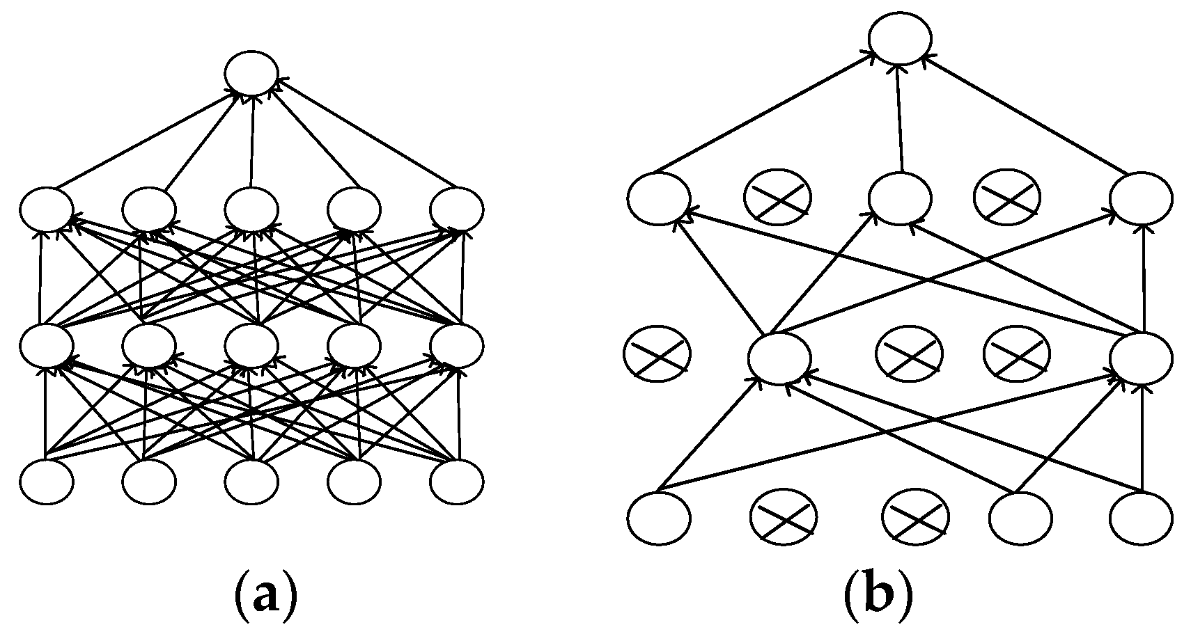
Dropout is a model average [20]. It is the weighted average of the estimated or predicted results from different models. The combinatorial estimate and the combinatorial prediction are the most commonly used methods. The random selection in the dropout may ignore the hidden layer nodes in the training process, consequently, each training network is different, and each training can be regarded as a new model. In particular, the hidden nodes randomly appear according to certain probabilities. Any two hidden nodes are not guaranteed to appear in the model multiple times simultaneously; thus, the updating of weights does not depend on the interaction of the implicit nodes of the fixed relation and can avoid the possible dependence of several features on another particular feature. Figure 2 compares neural network units with and without dropout layers. The nodes in each layer in the middle of Figure 2a may be associated with any node in the other layer, and some of the nodes in Figure 2b may be randomly ignored. These ignored, hidden layer nodes can reduce the cost of calculation. Moreover, these nodes can weaken the coupling between the nodes to reduce overfitting, thus becoming conducive to discovering the most essential characteristics of the data.
3. Modified CNN Based on Dropout and the SGD Optimizer
3.1. Quadratic CNN Structure
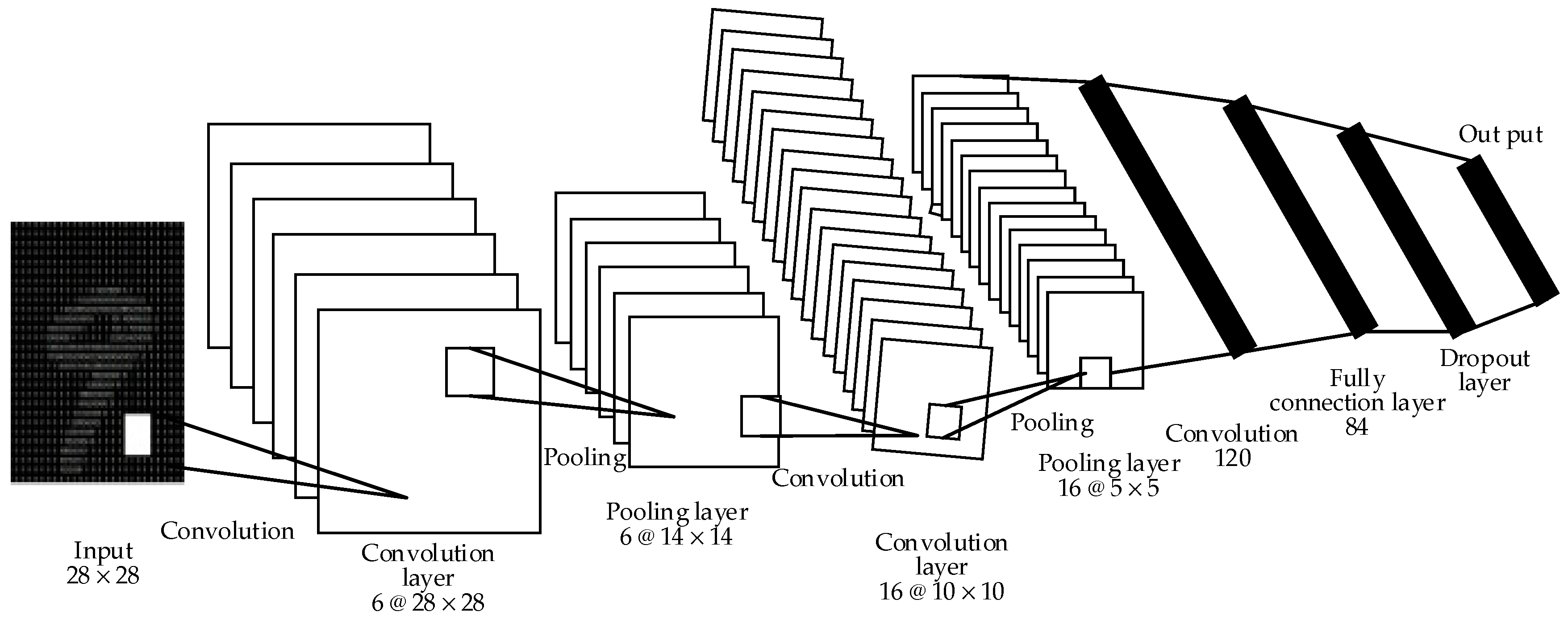
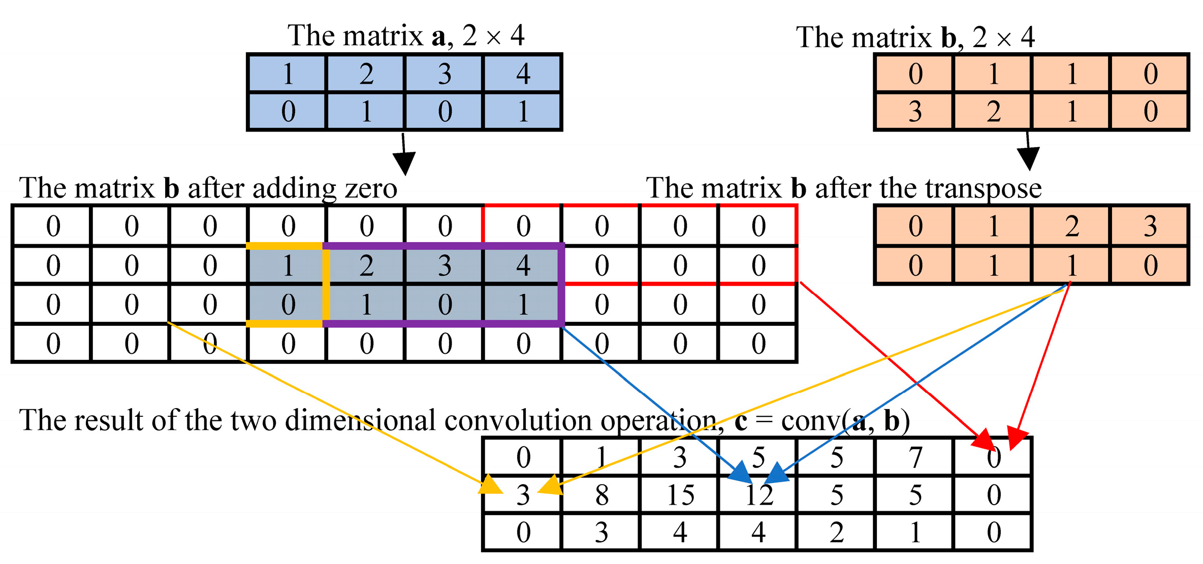
This study constructs the nine-layer CNN model, as shown in Figure 3, which contains an input layer, five hidden layers composed of convolution and pool layers, a fully connected layer, and an output layer (softmax). In this structure, a dropout layer comes after the fully connected layer. The probability of the neuron node in the test is p = 0.5 in the training phase, and p = 1 in the trial phase. The activation functions of the layers, except the output, are all rectified linear unit (Leaky ReLU) functions. The two-dimensional convolution operation is carried out by Conv2d function. The calculation illustration is shown in Figure 4.
The pooling operation (max pooling) is calculated using Formula (5).
where w(l)i,j represents the weight of the i neuron in the j class of the l layer; bi represents the offset of the i class; * represents the convolution operation; represents the output of j neurons in the l layer convolution; represents the output of the neuron in the layer, i.e., the input data for the layer; and represents the activation function of the model that has nonlinear characteristics.
3.2. Activation Function Based on Leaky ReLU
A traditional CNN often uses nonlinear functions, such as Tanh [21], ReLU [22], and Sigmoid [4], shown in Figure 5, to become an activation function.
The sigmoid function, which maps a real number input to the [0, 1] scope, encounters two problems as an activation function. (1) Gradient saturation: When the function activation value approaches the extremum 0 or 1, the gradient of the function tends to become 0. For the cost of the reverse propagation of the l layer neurons , the formula is , where (w(l))T represents the weight of the l neurons in the t layer. When the neuron reverse propagation cost in the l + 1 layer approaches 0, the computed gradient also approaches 0 to achieve the goal of not adjusting the update parameters. (2) Constantly positive weight: The average value of the function output is not 0, which causes the neuron layer to yield the signal input of the nonzero mean. This activity makes the data of the input neuron positive. Consequently, the weight becomes positive. These problems result in a slow parameter convergence and affect training efficiency and the model recognition effect. The tanh function can map a real input into the [−1, 1] range but it is actually a variant of the sigmoid function, i.e., . Moreover, the tanh function also exhibits the gradient saturation problem.
The ReLU function f(x) = max(0, x) (x ∈ (0, +∞)) (Figure 5c) has the following features. (1) Unsaturated gradient: The formula for the gradient is . Therefore, the problem of gradient dispersion in the reverse propagation process is alleviated, and the parameters in the first layer of the neural network can be updated rapidly. (2) Low computational complexity: The ReLU function sets the thresholds, i.e., if, x < 0 then f(x) = 0; if x > 0, then f(x) = x. Unfortunately, ReLU units can be fragile during training and can “die” [23]. A “dead” ReLU always outputs the same value.
The Leaky ReLUs activation function [24] with a small positive gradient for negative inputs was designed to solve the “dead” problem of ReLU. The formula of the Leaky ReLU is , which has all the advantages of the ReLU activation function but without the “dead” problem.
This study uses the Leaky ReLU function as the activation function because of its advantages to solve the gradient saturation problem and improve convergence speed.
3.3. Method Based on Dropout and SGD for Preventing Overfitting
The dropout is introduced into the CNN to improve the normalization capability of the network. Any neuron in a neural network is temporarily discarded by the probability p, and the formula is as follows:
To train the model, any indicator that makes the model “bad” is defined as a cost and cross entropy is used as the cost function , which is defined as follows:
where is the predicted probability distribution and is the actual distribution. In the model training phase, the SGD optimizer is used to optimize the cross entropy at different learning rates.
3.4. Modified Convolutional Neural Network Based on Dropout and the SGD Optimizer
On the basis of the design of the CNN structure, the Leaky ReLU activation function, and the overfitting prevention method that is based on dropout and the SGD, the Modified Convolutional Neural Network based on Dropout and the SGD Optimizer (MCNN-DS) is developed, which has the following main processes.
- Step 1: Pretrain the filter, and initialize the filter size pixel as P1 × P2.
- Step 2: Enter the image dataset for training. Process the image of the training set into the same picture as the filter size, and read the data to form the image data matrix X.
- Step 3: Initialize the weight w(l)i,j and bias bi and invoke the kernel function def Kernel() provided by TensorFlow to initialize parallel operations.
- Step 4: The Conv2d is used for two-dimensional convolution operation to obtain the first layer convolution feature matrix X(1).
- Step 5: The first layer convolution feature matrix X(1) is used as the input data of the pool layer. Use Formula (5) for the pool operation to obtain the feature matrix X(2).
- Step 6: Use the SGD optimizer function expressed in Formula (4) to derive the learning rate of the top-down tuning optimizer, and use the weights in TensorFlow and the update-biased interface to update the weight wi and the bias bi, thus obtaining the feature matrix X(3).
- Step 7: Generate the second convolution following Steps 4, 5, and 6 to derive the feature matrix X(4).
- Step 8: Merge the feature matrix X(4) into a column vector as the input of the neuron at the full-joint layer, multiply it with the weight matrix plus the bias, and then use the Leaky ReLU activation function to obtain the eigenvector b1.
- Step 9: Use the eigenvector of the fully connected stratum as the input of the dropout layer, compute the output probability of the neuron in the dropout layer using Formula (6), and the eigenvector b2 is obtained.
- Step 10: Use the eigenvector b2 as the input and the Softmax classifier [25] output to achieve the results.
Of note, in the convolution feature calculation for step 4 and step 5, the step length is 2 and the margin is set to 0. The pooling operation uses a 3 × 3 matrix on the basis of a policy previously presented in the literature [26] to ensure that the image input and output after feature extraction have the same size. The Leaky ReLU activation function is used in each step to activate the neuron.
4. Experiment and Analysis
4.1. Test Environment
The Python programming language is used in a 64-bit Ubuntu 16.04.4 implemented with the quadratic CNN learning algorithm. TensorFlow 1.5.0 is installed to evaluate the performance of the designed algorithm. Under various SGD learning rates, the performance of the CNN algorithm based on dropout and the SGD optimizer is tested, analyzed, and compared with that of four other algorithms. The results are measured on the same model computers purchased in multiple batches of the same batch and configured as follows: NVIDIA, GEFORCE GTX1080, with 8 GB internal storage.
4.2. Comparison Algorithm
The details of the four algorithms used for comparison are as follows.
- (1)
- Algorithm 1: weighted CNN (WCNN) [11]. This algorithm uses a sigmoid function as the activation function through compounded multiple convolutions and pooling layers to achieve input signal processing. Simultaneously, the mapping relationship between the connection layer and output target is established and the clustering algorithm is used to classify the feature.
- (2)
- Algorithm 2: convolutional neural network with fully connected Multilayer perceptron (MLP) (MLP-CNN) [6]. This algorithm improves model performance by increasing the characteristic number of the neural networks and using the stochastic gradient descent algorithm to optimize the cross entropy.
- (3)
- Algorithm 3: extreme learning machine (ELM) for multi-classification called SVM-ELM(ELM optimized with support vector machine) [27]. This calculation combines the fast learning machine and SVM, reduces the number of hidden nodes as a class number, and optimizes the linear decision function of each node through the SVM.
The structures of WCNN, MLP-CNN, and SVM-ELM are shown in Figure 6.
4.3. Datasets and Settings
The dataset used in the test includes three categories: MNIST handwritten numeral sets, HCL2000 handwritten Chinese character datasets, and EnglishHand handwritten alphabet datasets, all of which are grayscale images, as shown in Figure 7 (Table 1). MNIST was established by the National Institute of Standards and Technology for the study of handwritten numeral recognition and contains 60,000 training samples and 10,000 test samples, each with 28 px × 28 px BMP images. HCL2000 is a national standard database of off-line handwritten Chinese characters established by the Beijing University of Posts and Telecommunications, funded by the National 863 Program, and it collects 1300 written handwritings for 3755 first-level Chinese characters to form 1300 × 3755 samples. Each Chinese character has a sample of a 64 px × 64 px two-valued pixel. In this experiment, 3000 Chinese characters are randomly selected to form the training or test set, which is divided into 10 categories. The dataset is then adjusted to 28 px × 28 px size, and the pixel is normalized to [0,1]. EnglishHand is a public, handwritten alphabet dataset downloaded from the network (https://pan.baidu.com/s/1jJPtPSa). It mainly consists of 2860 lowercase letters and 2860 uppercase data samples, which are divided into 26 categories.
The 60,000 test samples and 10,000 training samples selected from the MNIST dataset are divided into 10 categories, i.e., 0–9 for a total of 10 characters corresponding to the training and test sets. The 2000 test samples and 1000 training samples selected from the HCL2000 dataset are divided into 10 categories, i.e., each Chinese character corresponds to the training and the test sets. The 1520 test samples and 5200 training samples selected from the EnglishHand dataset are divided into 26 categories, i.e., each alphabet character corresponds to the training and test sets. The volume kernel size of the convolution layer is 7 × 7 and 5 × 5, the pool factor is 3 × 3, the maximum number of iterations is 20,000, and the number of experiments is 10 times. The dropouts in the training and test phases have probabilities of p = 0.5 and p = 1, respectively.
4.4. Experimental Results and Analysis of Recognition Performance under Different Learning Rates
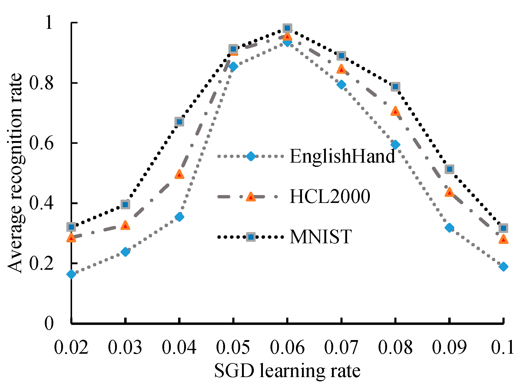
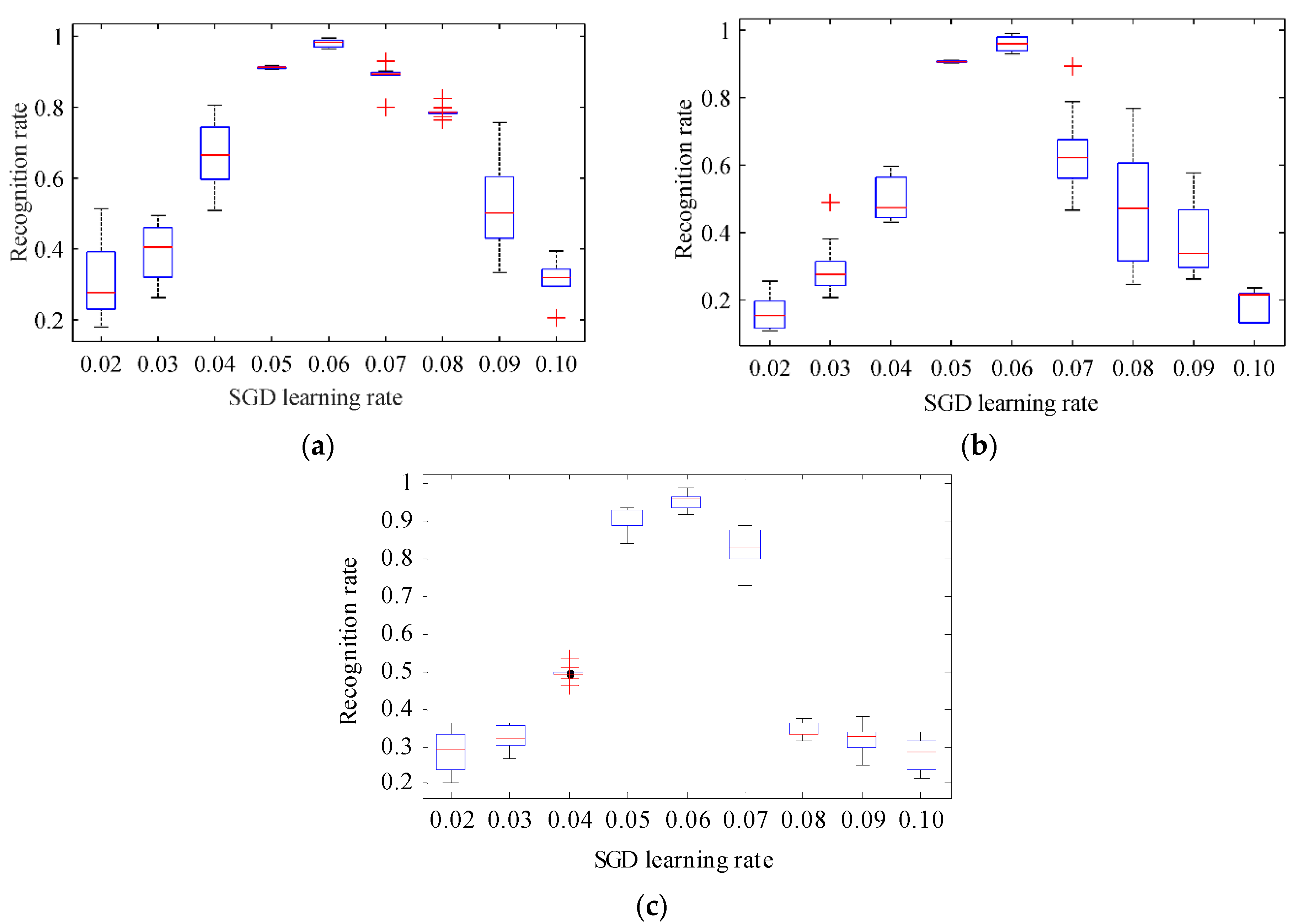
According to the experimental settings presented in the previous section, a different learning rate is provided to test the performance of the algorithm and determine the influences of the various learning rates of the SGD optimizer on the performance of the algorithm. The SGD optimizer minimizes the cross entropy learning rate, set to 0.02, 0.03, 0.04, 0.05, 0.06, 0.07, 0.08, 0.09, and 0.10. The statistical results and the boxplot of the recognition rate under each of the 10-time learning rates are shown in Figure 8 and Figure 9.
For the three datasets tested, the recognition rate of the model increases with the learning rate and the learning and recognition rates show a positive correlation when learning is in the [0.02, 0.05] range (Figure 8). When the learning rate distribution of the SGD optimizer is 0.05–0.07, the recognition rate of the model is in a relatively stable state. At this time, the recognition rate of the model shows a weak growth trend with the learning rate. When the learning rate is increased to more than 0.06, the recognition rate decreases significantly with any increase in learning rate. In particular, when the learning rate reaches 0.1, the recognition rate reaches the lowest level of approximately 20%. According to Figure 9, when the SGD learning rate is 0.06, the midline of the box diagram is higher and the rectangular area is the smallest, and it has no outliers. Analysis and testing based on three data sets show that tests conducted on this dataset show that the introduction of the SGD optimizer can affect the recognition rate. When the learning rate is 0.05–0.07, the performance of the system is enhanced. In the comparison experiment presented in the subsequent section, the learning rate of the SGD optimizer is set to 0.06.
4.5. Comparison and Analysis of the Three Kinds of Algorithms
The proposed algorithm runs 10 times for each test set. The recognition rates of the algorithms are shown in Table 2 and Figure 10. WCNN and MLP-CNN have no test results for the HCL2000 dataset. Thus, their data are not reflected in the figure. Table 3 is the time overhead of each algorithm on the test set. It is worth noting that because the algorithm WCNN does not give the result of the time overhead test, their data are not reflected in Table 3.
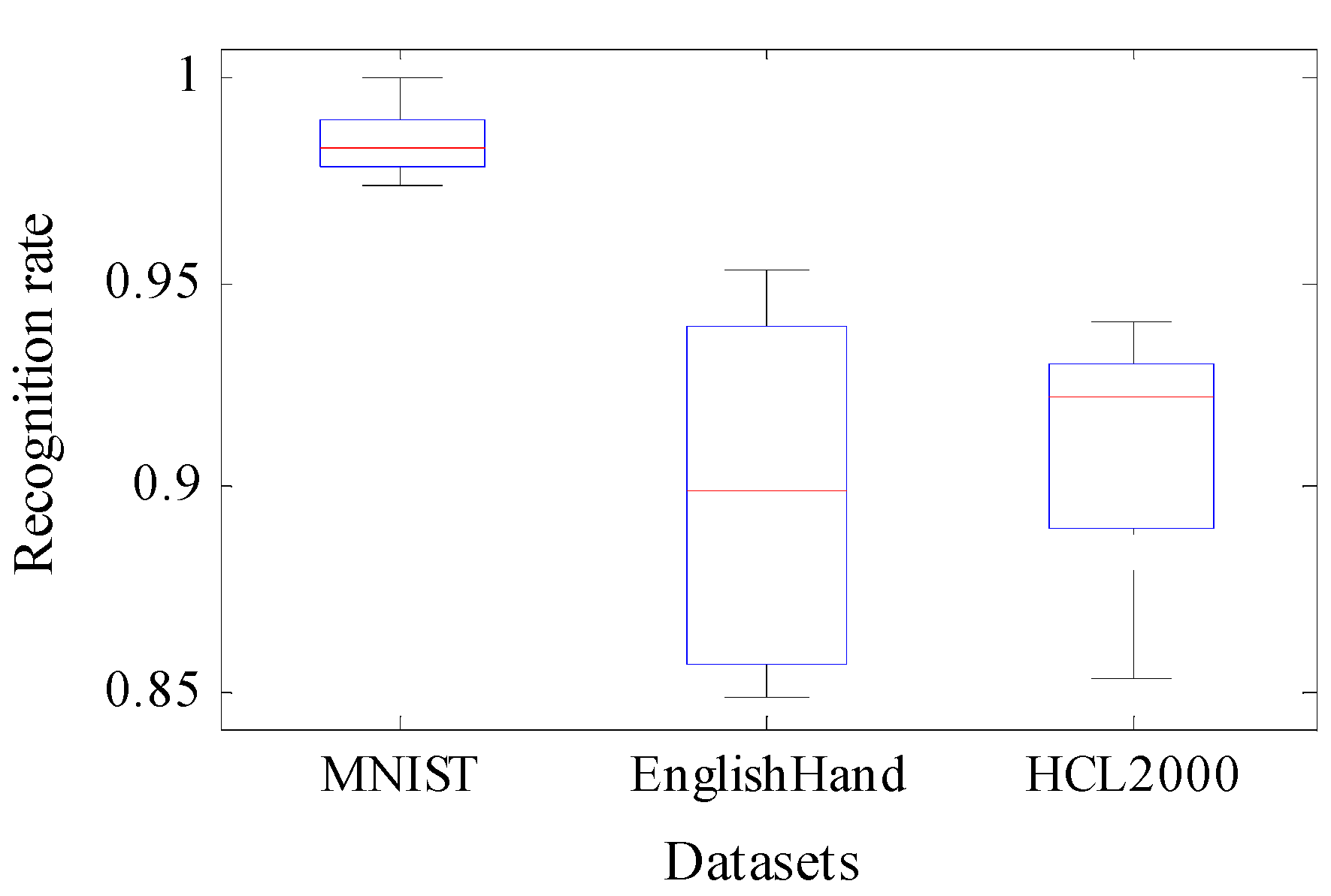
For the MNIST test set, the averages of WCNN, MLP-CNN, SVM-ELM, and the 10 operations of the proposed algorithm under the lowest recognition rate are 95.11%, 97.82%, 89.5%, and 97.36%, respectively (Table 2). In this study, the performance of the proposed algorithm ranks first, MLP-CNN ranks second, and SVM-ELM exhibits the worst performance. Under the highest and average recognition rates, the performance of the proposed algorithm ranks first, that of WCNN ranks second, and that of MLP-CNN shows the worst performance. According to the WCNN and MLP-CNN models and the performance of the proposed algorithm in feature recognition, our model is better than SVM-ELM in feature extraction and fusion even when it is the worst. Table 2 shows that the recognition rate of the proposed algorithm is the best, reaching a maximum of 99.97%. Furthermore, the average recognition rate of the MCNN-DS algorithm in the three databases is 98.4, 90.98, and 89.77, with a standard deviation of 0.0084, 0.0396, and 0.0280, respectively. The standard deviation is small and average recognition accuracy is high, which indicates that the MCNN-DS algorithm can stably extract abundant feature information. The algorithm also has the same advantage in terms of time to unlock precisely because of the implementation of the algorithm parallelization. Furthermore, the time-cost of this algorithm is merely 21.95% of the MLP-CNN algorithm, and 10.02% of the SVM-ELM algorithm.
Compared with the SVM-ELM algorithms, this algorithm has an advantage over the HCL2000 test set. The lowest recognition rate of the proposed model is 1.82% higher than that of SVM-ELM. The highest recognition rate of the algorithm is 3.99% higher than that of SVM-ELM. The average recognition rate of the algorithm is 2.35% higher than that of SVM-ELM. The time-cost of this algorithm is merely 15.41% of the SVM-ELM. For the EnglishHand test set, the lowest recognition rate of this algorithm is 84.93%, the highest recognition rate is 95.29%, the average recognition rate is 89.77%, and its time overhead is 21.617 s. In fact, the time of computations strongly rely on the number of layers and connections, and SGD follows the negative gradient of the objective after checking only a single or some training examples. It is because the change of the structure, the use of the Leaky ReLU activation function, and the overfitting prevention method based on Dropout and SGD result in the acceleration.
In summary, the algorithm proposed in this study is robust and superior to the algorithms used for comparison in terms of recognition, time-cost, and rate.
5. Conclusions
To improve the accuracy of feature extraction while reducing time-cost, this study investigates the structure of the CNN, the overfitting problem, and combines dropout and the SGD optimizer with the CNN. An improved CNN algorithm based on dropout and the SGD optimizer is proposed, and parallelization is achieved using TensorFlow. The use of SGD leads the MCNN-DS to work faster because it does not use the whole training instances in each integration and can dynamically adjust the estimation of the first- and second-order matrices of the gradient of each parameter according to the loss function, which can reduce the amount of calculations and improve the computing speed. Furthermore, by improving the activation function, the algorithm avoids the problem of the neuron node output becoming 0, improves recognition accuracy, and reduces time-cost. As the present test dataset is limited, future studies need to use additional test sets to improve the performance of the algorithm. Moreover, the algorithm should be combined with the service robot system [28] established by the research group to conduct application research and to develop and improve model robustness. In addition, reducing the number of neurons in the CNN can lead to the reduction of computations at the working and testing stages; however, the dropout algorithm used at the learning stage increases the time of processing. We focused on improving the recognition accuracy at the beginning of the research. The time consumption of both stages requires further investigation.
Acknowledgments
This research was partially supported by the National Natural Science Foundation of China, under Grant 61640209 and 91746116, the Foundation for Distinguished Young Talents of Guizhou Province, under grant QKHRZ[2015]13, the Science and Technology Foundation of Guizhou Province under grant JZ[2014]2004, JZ[2014]2001, ZDZX[2013]6020, and LH[2016]7433, and the Basic Platform Program of Guizhou Province under grant QKHPTRC[2018]5702 and [2017]5788.
Author Contributions
Guanci Yang conceived of and designed the study. Jing Yang made substantial contributions to the implementation of the algorithm and analysis of the data. The manuscript was written by Guanci Yang with contributions from all the authors. All the authors read and approved the submitted manuscript, agreed to be listed, and accepted this version for publication.
Conflicts of Interest
The authors declare no conflict of interest.
References
- Vieira, S.; Pinaya, W.H.L.; Mechelli, A. Using deep learning to investigate the neuroimaging correlates of psychiatric and neurological disorders: Methods and applications. Neurosci. Biobehav. Rev. 2017, 74, 58–75. [Google Scholar] [CrossRef] [PubMed]
- Li, S.; Dou, Y.; Niu, X.; Lv, Q.; Wang, Q. A Fast and Memory Saved GPU Acceleration Algorithm of Convolutional Neural Networks for Target Detection. Neurocomputing 2017, 230, 48–59. [Google Scholar] [CrossRef]
- Gong, T.; Fan, T.; Guo, J.; Cai, Z. GPU-based parallel optimization of immune convolutional neural network and embedded system. Eng. Appl. Artif. Intell. 2016, 36, 226–238. [Google Scholar] [CrossRef]
- Zhang, Y.N.; Qu, L.; Chen, J.W.; Liu, J.R.; Guo, D.S. Weights and structure determination method of multiple-input Sigmoid activation function neural network. Appl. Res. Comput. 2012, 29, 4113–4116. [Google Scholar]
- Chen, L.; Wu, C.; Fan, W.; Sun, J.; Naoi, S. Adaptive Local Receptive Field Convolutional Neural Networks for Handwritten Chinese Character Recognition. In Chinese Conference on Pattern Recognition; Springer: Berlin/Heidelberg, Germany, 2014; pp. 455–463. [Google Scholar]
- Singh, P.; Verma, A.; Chaudhari, N.S. Deep Convolutional Neural Network Classifier for Handwritten Devanagari Character Recognition. In Information Systems Design and Intelligent Applications; Springer: New Delhi, India, 2016. [Google Scholar]
- Sun, W.; Su, F. A novel companion objective function for regularization of deepconvolutional neural networks. Image Vis. Comput. 2016, 56, 110–126. [Google Scholar]
- Wachinger, C.; Reuter, M.; Klein, T. DeepNAT: Deep convolutional neural network for segmenting neuroanatomy. NeuroImage 2017. [Google Scholar] [CrossRef] [PubMed]
- Chen, L.C.; Papandreou, G.; Kokkinos, I.; Murphy, K.; Yuille, A.L. Semantic Image Segmentation with Deep Convolutional Nets and Fully Connected CRFs. Comput. Sci. 2016, 26, 357–361. [Google Scholar]
- Izotov, P.Y.; Kazanskiy, N.L.; Golovashkin, D.L.; Sukhanov, S.V. CUDA-enabled implementation of a neural network algorithm for handwritten digit recognition. Opt. Mem. Neural Netw. 2011, 20, 98–106. [Google Scholar] [CrossRef]
- Hao, H.W.; Jiang, R.R. Training sample selection method for Neural Networks based on Nearest neighbor rule. Acta Autom. Sin. 2007, 33, 1247–1251. [Google Scholar]
- Akeret, J.; Chang, C.; Lucchi, A.; Refregier, A. Radio frequency interference mitigation using deep convolutional neural networks. Astron. Comput. 2017, 18, 35–39. [Google Scholar] [CrossRef]
- Costarelli, D.; Vinti, G. Pointwise and uniform approximation by multivariate neural network operators of the max-product type. Neural Netw. 2016, 81, 81–90. [Google Scholar] [CrossRef] [PubMed]
- Lee, C.Y.; Xie, S.; Gallagher, P.; Zhang, Z.; Tu, Z. Deeply-supervised nets. In Proceedings of the Eighteenth International Conference on Artificial Intelligence and Statistics, San Diego, CA, USA, 21 February 2015; pp. 562–570. [Google Scholar]
- LeCun, Y.; Bottou, L.; Bengio, Y.; Haffner, P. Gradient-based learning applied to document recognition. Proc. IEEE 1998, 86, 2278–2323. [Google Scholar] [CrossRef]
- Zhou, F.-Y.; Jin, L.-P.; Dong, J. Review of Convolutional Neural Network. Chin. J. Comput. 2017, 40, 1229–1251. [Google Scholar] [CrossRef]
- Najafabadi, M.M.; Khoshgoftaar, T.M.; Villanustre, F.; Holt, J. Large-scale distributed L-BFGS. J. Big Data 2017, 4, 22. [Google Scholar] [CrossRef]
- Zinkevich, M.; Weimer, M.; Li, L.; Smola, A.J. Parallelized stochastic gradient descent. In Advances in Neural Information Processing Systems; Neural Information Processing Systems Foundation, Inc.: La Jolla, CA, USA, 2010; pp. 2595–2603. [Google Scholar]
- Hardt, M.; Recht, B.; Singer, Y. Train faster, generalize better: Stability of stochastic gradient descent. arXiv, 2015; arXiv:1509.01240. [Google Scholar]
- Hou, Z.H.; Fang, H.J. Robust fault-tolerant control for networked control system with packet dropout. J. Syst. Eng. Electron. 2007, 18, 76–82. [Google Scholar]
- Luo, P.; Li, H.F. Research on Quantum Neural Network and its Applications Based on Tanh Activation Function. Comput. Digit. Eng. 2012, 16, 33–39. [Google Scholar] [CrossRef]
- Tang, Z.; Luo, L.; Peng, H.; Li, S. A joint residual network with paired ReLUs activation for image super-resolution. Neurocomputing 2018, 273, 37–46. [Google Scholar] [CrossRef]
- Günnemann, N.; Pfeffer, J. Predicting Defective Engines using Convolutional Neural Networks on Temporal Vibration Signals. In Proceedings of the First International Workshop on Learning with Imbalanced Domains: Theory and Applications, Munich, Germany, 11 October 2017; pp. 92–102. [Google Scholar]
- Jin, X.; Xu, C.; Feng, J.; Wei, Y.; Xiong, J.; Yan, S. Deep learning with S-shaped rectified linear activation units. In Proceedings of the Thirtieth AAAI Conference on Artificial Intelligence (AAAI Press), Phoenix, AZ, USA, 12–17 February 2016; pp. 1737–1743. [Google Scholar]
- Shi, X.B.; Fang, X.J.; Zhang, D.Y.; Guo, Z.Q. Image Classification Based on Mixed Deep Learning Model Transfer Learning. J. Syst. Simul. 2016, 28, 167–173. [Google Scholar]
- Yang, W.; Jin, L.; Tao, D.; Xie, Z.; Feng, Z. DropSample: A new training method to enhance deep convolutional neural networks for large-scale unconstrained handwritten Chinese character recognition. Pattern Recognit. 2016, 58, 190–203. [Google Scholar] [CrossRef]
- Shen, F.; Wang, L.; Zhang, J. Reduced extreme learning machine employing SVM technique. J. Huazhong Univ. Sci. Technol. 2014, 42, 107–110. [Google Scholar] [CrossRef]
- Yang, G.-C.; Yang, J.; Su, Z.D.; Chen, Z.-J. Improved YOLO feature extraction algorithm and its application to privacy situation detection of social robots. Acta Autom. Sin. 2018, 1–12. [Google Scholar] [CrossRef]
Figure 1.
Traditional convolutional neural network structure diagram.
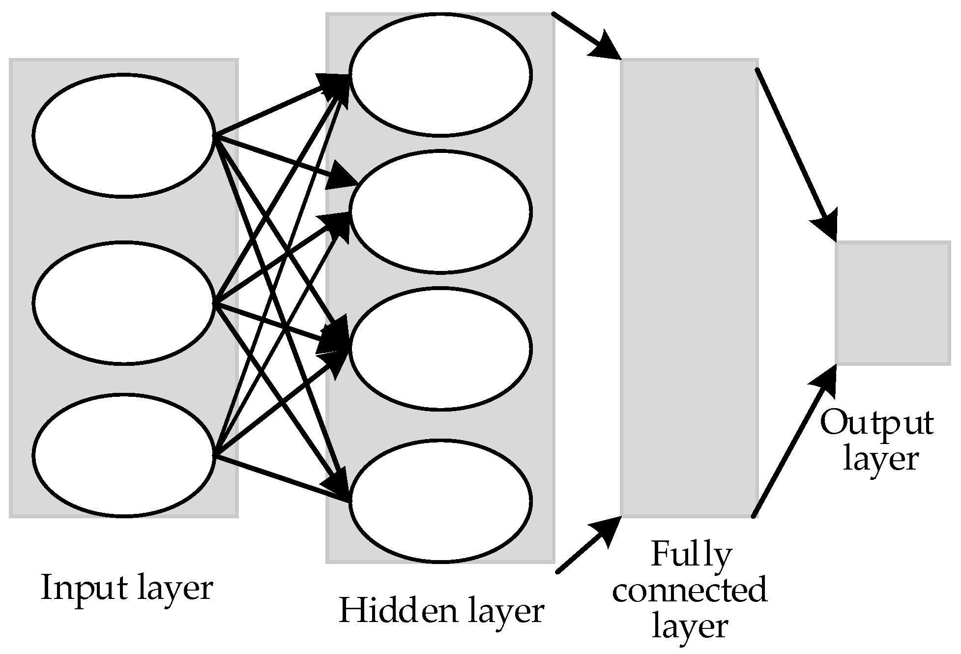
Figure 2.
Neural network unit connections with different mechanisms. (a) Without the dropout layer mechanism; (b) With the dropout layer mechanism.
Figure 2.
Neural network unit connections with different mechanisms. (a) Without the dropout layer mechanism; (b) With the dropout layer mechanism.

Figure 3.
Quadratic convolution neural network structure model.

Figure 4.
Illustration of the two-dimensional convolution operation process.

Figure 5.
Nonlinear function. (a) Sigmoid function; (b) Tanh function; (c) ReLU function; (d) Leaky ReLU function.
Figure 5.
Nonlinear function. (a) Sigmoid function; (b) Tanh function; (c) ReLU function; (d) Leaky ReLU function.
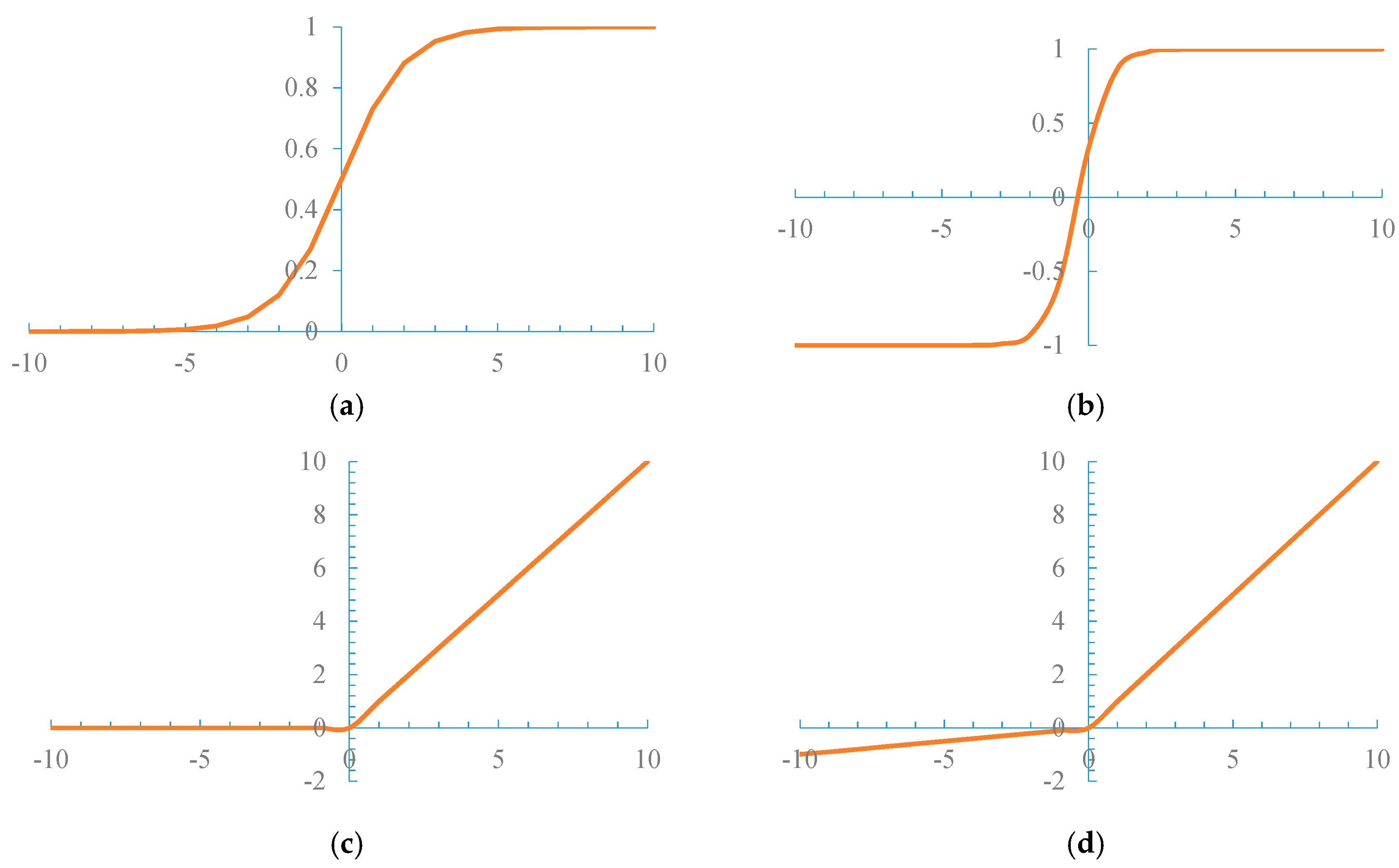
Figure 6.
Convolution neural network structure model of comparison algorithms. (a) WCNN; (b) MLP-CNN; (c) SVM-ELM.
Figure 6.
Convolution neural network structure model of comparison algorithms. (a) WCNN; (b) MLP-CNN; (c) SVM-ELM.
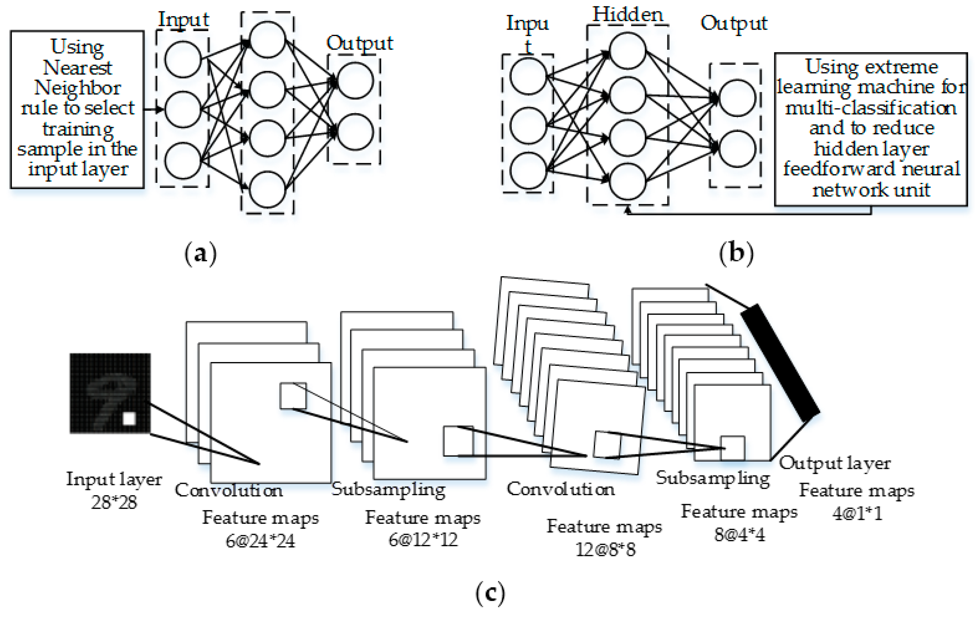
Figure 7.
Sample of handwriting character images. (a) MNIST dataset; (b) HCL2000 dataset; (c) EnglishHand dataset.
Figure 7.
Sample of handwriting character images. (a) MNIST dataset; (b) HCL2000 dataset; (c) EnglishHand dataset.
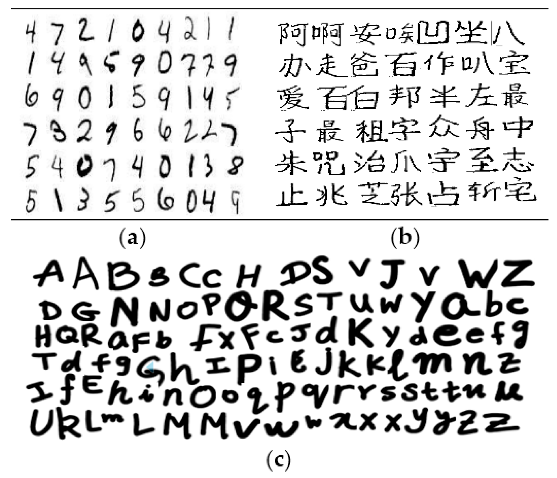
Figure 8.
Recognition value under different stochastic gradient descent (SGD) learning rates.

Figure 9.
Boxplot of the recognition rate obtained by MCNN-DS under different SGD learning rates. (a) MNIST dataset; (b) EnglishHand dataset; (c) HCL2000 dataset.
Figure 9.
Boxplot of the recognition rate obtained by MCNN-DS under different SGD learning rates. (a) MNIST dataset; (b) EnglishHand dataset; (c) HCL2000 dataset.

Figure 10.
Boxplot of the recognition rate obtained by MCNN-DS.

Table 1.
Test and training datasets.
| Datasets | Size of Training Set | Size of Test Set | Number of Image Category |
|---|---|---|---|
| MNIST | 60,000 | 10,000 | 10 |
| HCL2000 | 2000 | 1000 | 10 |
| EnglishHand | 4200 | 1520 | 26 |
Table 2.
Algorithm recognition performance comparison.
| Dataset | Metric | WCNN [11] | MLP-CNN [6] | SVM-ELM [27] | MCNN-DS |
|---|---|---|---|---|---|
| MNIST | The lowest recognition rate (%) | 95.11 | 97.82 | 89.5 | 97.36 |
| The highest recognition rate (%) | 95.71 | 98.96 | 91.35 | 99.97 | |
| The average recognition rate (%) | 95.36 | 96.32 | 90.26 | 98.43 | |
| Standard deviation of recognition rate | -- | -- | -- | 0.0084 | |
| HCL2000 | The lowest recognition rate (%) | -- | -- | 83.60 | 85.42 |
| The highest recognition rate (%) | -- | -- | 90.00 | 93.99 | |
| The average recognition rate (%) | -- | -- | 88.63 | 90.98 | |
| Standard deviation of recognition rate | -- | -- | -- | 0.0396 | |
| EnglishHand | The lowest recognition rate (%) | -- | -- | -- | 84.93 |
| The highest recognition rate (%) | -- | -- | -- | 95.29 | |
| The average recognition rate (%) | -- | -- | -- | 89.77 | |
| Standard deviation of recognition rate | -- | -- | -- | 0.0280 |
Table 3.
Statistic results of time overhead.
| Algorithms | Time/ms | ||
|---|---|---|---|
| MNIST | HCL2000 | EnglishHand | |
| MLP-CNN | 290,491 | -- | -- |
| SVM-ELM | 132,634 | 316,372 | -- |
| MCNN-DS | 13,236 | 20,531 | 21,617 |
© 2018 by the authors. Licensee MDPI, Basel, Switzerland. This article is an open access article distributed under the terms and conditions of the Creative Commons Attribution (CC BY) license (http://creativecommons.org/licenses/by/4.0/).
Share and Cite
MDPI and ACS Style
Yang, J.; Yang, G. Modified Convolutional Neural Network Based on Dropout and the Stochastic Gradient Descent Optimizer. Algorithms 2018, 11, 28. https://doi.org/10.3390/a11030028
AMA Style
Yang J, Yang G. Modified Convolutional Neural Network Based on Dropout and the Stochastic Gradient Descent Optimizer. Algorithms. 2018; 11(3):28. https://doi.org/10.3390/a11030028
Chicago/Turabian StyleYang, Jing, and Guanci Yang. 2018. "Modified Convolutional Neural Network Based on Dropout and the Stochastic Gradient Descent Optimizer" Algorithms 11, no. 3: 28. https://doi.org/10.3390/a11030028
Note that from the first issue of 2016, this journal uses article numbers instead of page numbers. See further details here.