Bilayer Local Search Enhanced Particle Swarm Optimization for the Capacitated Vehicle Routing Problem


Department of Industrial and Management Engineering, Hankuk University of Foreign Studies, Yongin 17035, Korea
*
Author to whom correspondence should be addressed.
Algorithms 2018, 11(3), 31; https://doi.org/10.3390/a11030031
Submission received: 29 January 2018
/
Revised: 7 March 2018
/
Accepted: 13 March 2018
/
Published: 15 March 2018
(This article belongs to the Special Issue Metaheuristics for Rich Vehicle Routing Problems)
Abstract
:The classical capacitated vehicle routing problem (CVRP) is a very popular combinatorial optimization problem in the field of logistics and supply chain management. Although CVRP has drawn interests of many researchers, no standard way has been established yet to obtain best known solutions for all the different problem sets. We propose an efficient algorithm Bilayer Local Search-based Particle Swarm Optimization (BLS-PSO) along with a novel decoding method to solve CVRP. Decoding method is important to relate the encoded particle position to a feasible CVRP solution. In bilayer local search, one layer of local search is for the whole population in any iteration whereas another one is applied only on the pool of the best particles generated in different generations. Such searching strategies help the BLS-PSO to perform better than the existing proposals by obtaining best known solutions for most of the existing benchmark problems within very reasonable computational time. Computational results also show that the performance achieved by the proposed algorithm outperforms other PSO-based approaches.
1. Introduction
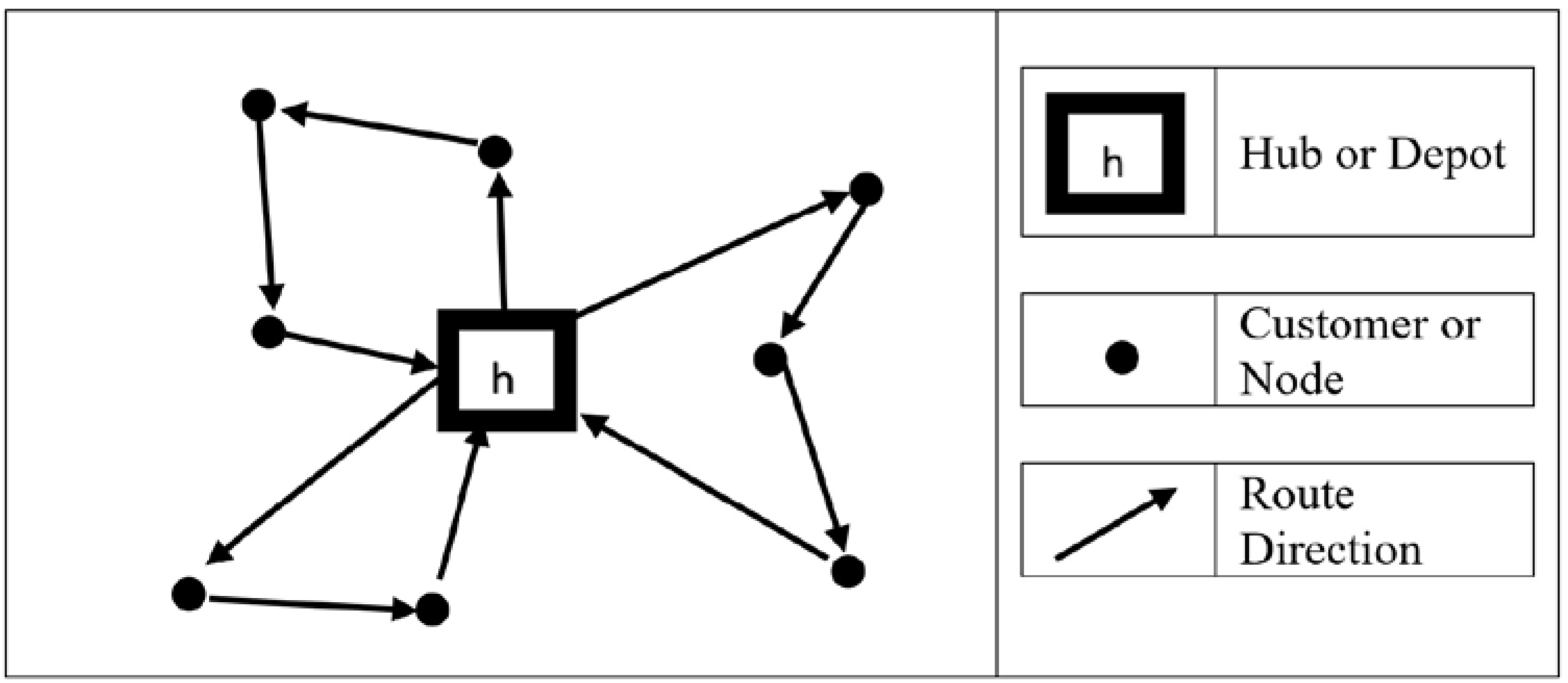
The huge importance of solving capacitated vehicle routing problem (CVRP) in companies supporting service and logistics for supplying commodities is a strong motivation for many researchers worldwide to solve the CVRP with innovative algorithms. Capacitated Vehicle Routing Problem in general deals with some customer nodes having some sort of pre-specified demands to be served from a hub with a set of vehicles. Although there are many practical constraints in the real world like stochastic customer demand, resource restrictions and so on. There are many pieces of research that introduce practical variations of CVRP [1,2,3,4,5]. However, a large portion of practical applications are simple in nature which can be fit to CVRP. The definition of CVRP has been outlined in [6]. A vehicle picks some shipment from the depot to serve some of the customers according to their demands until its capacity permits, makes a trip to serve them, and returns to the depot. The vehicles also have additional restrictions on their maximum travelling distance which is the total of distance travelled by the vehicle and the service time it requires to handle the customers it serves. A set of nodes is given on a graph and a hub location h is specified among them. Then a vehicle routing problem can be portrayed as Figure 1, where the nodes represent customers, cities or so on. The target of solving a CVRP is to find minimum total cost, specifically minimum travelling distance, incurred by the vehicles for visiting the customer nodes to satisfy their demands.
CVRP is closely related to the classical Travelling Salesperson’s Problem (TSP) with a difference that vehicle capacity is limited in CVRP, but not in TSP. This makes CVRP a more complex problem than TSP. As TSP is a well-known NP hard problem, where no algorithm is available to solve TSP by polynomial time when the number of nodes increases, CVRP too is obviously an NP hard problem [7].
Even though an exact algorithm is unlikely to exist to solve CVRP, there have been a few attempts from researchers based on branch and bound technique, set partitioning technique and so on, which can handle CVRP with only few nodes [8]. Therefore, many approximate algorithms are proposed to solve CVRP effectively. Although these algorithms never find the optimal, they can find “good” or near-optimal solutions within a reasonable computational time.
Among heuristics, Clark and Wright’s saving algorithm is a very early introduction in the area of CVRP [9]. This technique is basically a constructive heuristic which builds tours gradually by inserting a node at each time with respect to some saving conditions till no more cluster can be constructed. There are many improvements and variations available in the literature from many researchers [10,11,12]. “Cluster-First Route-Second” [13,14] and “Route-First Cluster-Second” [15] are other two well-known algorithms for handling CVRP. The former one builds some clusters of customers then a TSP tour is obtained with those customers to solve CVRP, and the latter one is the technique to make a TSP tour of all customers then cluster them into routes with respect to the given constraints.
Recently many nature-inspired metaheuristics such as Genetic Algorithm (GA) [16,17], Tabu Search (TS) [18,19,20] and Simulated Annealing (SA) [21,22] have become attractive in the field of optimization. Nevertheless, there are many research articles that report their performances in dealing with CVRP [23,24,25,26,27]. It is worth mentioning that swarm optimization techniques are getting popular due to their simplicity and performance to handle optimization problems nowadays [28,29,30]. Swarm-based metaheuristics are mainly inspired from unique characteristics of some swarms such as birds (bird flocking), fish (fish schooling), ants (foraging), etc. These creatures are not very intelligent individually whereas they show intelligent and complex behavior while working collectively; see, for example, the foraging behavior of bees for honey collection. Swarm-based metaheuristics are also getting remarkable attention from many researchers in dealing optimization problems like CVRP and its variations [31,32,33,34,35,36,37].
In this work, to explain the applicability of the proposed scheme, we adopt particle swarm optimization (PSO) due to its growing applications in the field of optimization [38,39]. PSO was first introduced by Kennedy and Eberhart [40] for handling continuous optimization problems. Afterwards, numerous applications are proposed to trick the discrete optimization problems till date. Among them, articles on CVRP are also available in the literature. Quantum individual-based discrete PSO (DPSO) is proposed in [41] where, the quantum particle swarm optimization is introduced in [42]. In DPSO, PSO is hybridized with simulated annealing (SA) to obtain a complete CVRP solution. In their approach they cluster the customers with DPSO, and then make a sequence of customers utilizing the SA algorithm. Though they show quality solutions for some benchmark instances, and the approach requires large computational time to reach the best-known solutions (BKS). Kao [43] proposed a combinatorial PSO mainly based on the work of Chen [41]. A technique utilizing an advanced version of PSO, namely GLN-PSO in [44], was introduced by Pongchairerks and Kachitvichyanukul [45]. They utilize two decoding techniques namely “Solution Representation-1 (SR-1)” and “Solution Representation-2 (SR-2)” to solve CVRP where the first decoding technique (SR-1) is an improved version of their previous work [46]. Mainly a local search is added to their previous solution representation which was a decoding technique based on relative position of vehicles. The second decoding technique (SR-2) is an enhanced version of SR-1 where they consider a vehicle coverage radius in addition to other two reference points for the vehicles in their representation. Even though Ai achieves better results [44] than their previous work [46], the computational time is still noticeable. A hybrid PSO is presented in [47] where they obtained initial solutions to run their PSO utilizing MPNS-GRASP [48]. To reduce the computational time, they utilize expanding neighborhood search [49,50] as well. They utilize path relinking technique [51] to guide the PSO. There is another hybrid approach in [52] which hybridizes two swarm optimization techniques, namely ACO and PSO. ACO mainly make clusters of customer and builds the routes, and then PSO is utilized in short term memory to speed up the convergence by laying pheromone on the global and personal best solutions only. However, these algorithms have shown some good results at the expense of considerable computational time as all the approaches are mainly devoted to obtaining optimal solutions to the problems rather than concentrating on the main idea of approximation algorithms which is to obtain good solutions for large problems within reasonable computational time.
A candidate solution represented by a particle in PSO is usually in an encoded form, which needs a decoding procedure to obtain the comprehensive meaning of it. In this article, we represent a solution in a simple vector form to easily apply different operations of PSO, and at the same time we propose an effective decoding algorithm to interpret the solution. Decoded results are then exploited with a unique bilayer local search scheme. One layer of local search is for each particle in every iteration. The second layer of local search is applied on the pool of the best particles generated in different generations. The local search scheme improves the solution very effectively. Addition of these simple steps makes the algorithm very fast as compared to other available techniques and shows remarkable results in handling benchmark problems.
The rest of the article is organized as follows. A clear formulation of the problem statement is presented in Section 2. The proposed bilayer local search-enhanced PSO (BLS-PSO) is introduced describing the methodology in detail in Section 3. Section 4 presents the parameter optimization, the discussion of computational results and the comparison with other best known PSO-based algorithms. Finally, conclusion and future remarks are made in Section 5.
2. Mathematical Formulation
CVRP is usually stated as a graph of a set C = {ci|i = 1, 2, …, n} of n nodes, resembling customers, along with associated demands D = {di|i = 1, 2, …, n} and required service times ST = {sti|i = 1, 2, …, n}. If no service time is specified for the customers in a problem definition, then it is set to 0. Among the nodes, a special node, say ch, is called the depot, from where the demands of other nodes are met using some vehicles. For the depot ch, the service time sth = 0. A vehicle starts from the depot, serves the demands of some nodes, and comes back to the depot. The objective is to serve all the customers using a set of vehicles, keeping the cost (usually calculated as the total distance travelled by the vehicles) as low as possible. A capacity constraint is associated with every vehicle, which specifies the maximum amount of total demands of the nodes that can be served by it. Maximum travel distance is another constraint that, if specified, puts a limit on the total distance traveled along with service time spent by a vehicle [43].
The required variables for the CVRP formulation are presented in Table 1.
Some notations and variables related to the formulation of CVRP are stated in Table 1, based on which the problem can be formulated as a minimization problem as
fulfilling the following constraints
Equations (2)–(8) are the constraints to ensure the validity of a solution to Equation (1). Equations (2) and (3) ensure that a customer is served by exactly one vehicle. Equation (4) ensures the direction of a vehicle to serve a node i.e., if a vehicle travels from node cj to node co then it never returns to the node co from any other node ck or depot ch. Equation (5) restricts the customers to be assigned to a vehicle exceeding the maximum load capacity of that vehicle. Equation (6) confirms the fulfillment of the maximum travel distance constraint of a vehicle. Equation (7) forces a vehicle to start the journey from and end at the depot ch and never visit the depot any more. Equation (8) restricts sub-tour generated within a route. Equation (9) is the integrality constraint for the formulation.
3. Proposed Methodology
The traditional PSO algorithm applies the velocities on the particles to explore new solutions. We propose an enhanced PSO by incorporating a bilayer local search approach with it. The first layer of local search is applied on the whole population, i.e., on each particle in the population in every iteration. Thus, it improves the quality of the solutions obtained by traditional PSO by searching their neighborhoods. The second layer of local search is implemented on the pool of the best particles found in different iterations. This layer is to give additional chances to the best particles to look for better solutions in their neighborhoods. Such local searches allow the particles to have a better exploration around the current position as otherwise a particle may move from a position missing out a nearby potential solution.
We represent a particle in PSO in an encoded vector form to apply PSO operations easily on them. Hence, we also propose a decoding method to build a real comprehensive solution out of a particle. The overall workflow of proposed bilayer local search-enhanced particle swarm optimization (BLS-PSO) is sketched in Figure 2.
The proposed BLS-PSO technique to solve a capacitated vehicle routing problem (CVRP) can broadly be thought as having three major parts: the application of the particle swarm optimization (PSO), the decoding step to obtain the detail routes encoded in a solution and the bilayer local search approach to search for a better solution in the neighborhood. We discuss these steps in detail in the following subsections.
3.1. PSO for CVRP
PSO is a population-based metaheuristic which consists of particles or chromosomes consisting of candidate solutions. In this work, a chromosome is a “Customer Vector”, a permutation of all the customers specified in a problem statement. We can also think such a customer vector as a position vector in the solution space.
At first, we generate a predetermined number of random particles for PSO. We also assign a random velocity for each particle to guide the particles to search for better solutions utilizing the PSO scheme. If the position of the l-th particle is on iteration (t − 1), then the particle can move to its new position influenced by its velocity , as done in the traditional PSO, using
The velocity also gets updated at each iteration, according to Shi and Eberhart [53], as
where is the velocity of the lth particle in the t-th iteration, Bl is the best solution attained by the l-th particle till (t − 1) iterations, and G is best solution attained by any particle in the population in (t − 1) iterations. k1, k2 and k3 are parameters to guide the velocity to move a particle to a certain direction specifying the effect of its own velocity, attraction to the best position ever reached by itself and the best position ever reached by any particle in the population. Effect of the history of velocity is controlled by the parameter k1, influence of the personal best position is determined by k2 and k3 maintains the balance with the global best solution at any stage. These influences are basically the strength of PSO algorithm which leads a particle to a better position. Thus, we have utilized the proposal of Shi and Eberhart [53] instead of using the straightforward PSO velocity update equation from Eberhart and Kennedy [40] to try to keep the preeminent balance among the influential portions in Equation (11).
PSO was first proposed for continuous problem domains where can be considered as vector addition and as vector subtraction. However, CVRP is defined in discrete domain. Hence, to apply PSO in discrete domain, we adopt the swap sequence-based PSO [54]. We need to map the meaning of Equations (10) and (11) so that PSO can deal a discrete type problem. In this purpose [54], authors proposed a new definition to the characteristics of two symbols, and . X SS means applying a sequence of swap sequence on the elements of X to reach Y, a new position in the solution space, while X W gives a basic swap sequence BSS, the applying of which W can be converted to X. A detailed description is presented here to understand the mechanism of the operators.
Swap sequence is basically moving a particle from one solution or position to another solution or position in the solution space. Suppose an encoded solution or particle in the solution space is X = (1, 3, 5, 2, 4) assuming the problem has five nodes in the problem statement. Then SS can be a swap sequence consisting of one or more swap operators that move X to its new position Y. For example SS = SO(2,3) may be a random initial swap sequence having a single swap operator or velocity for particle X. Thus, X SS = (1, 3, 5, 2, 4) SO(2, 3) = (1, 5, 3, 2, 4) would be Y the new particle position. However, SS may be a swap sequence having more than one swap sequence or basic swap sequence or swap operators as well. Let another SS = SO(2, 3) SO(4, 5) having two swap operators. Applying a swap sequence with more than one swap operators on a particle is simply applying swap operators one after another on the particle. Thus, X SS = (1, 3, 5, 2, 4) SO(2, 3) SO(4, 5) = (1, 5, 3, 2, 4) SO(4, 5) = (1, 5, 3, 4, 2). This definition helps to make a swap sequence or velocity from Equation (11) and then swap sequence will apply on a particle according to Equation (10) to move the particle from one position to other.
Another definition of BSS is basically the difference between two positions in a solution space to relate the personal best position or global best position with present position of a particle. In other words, BSS = X W. Suppose X = (1, 3, 5, 2, 4) and W = (5, 1, 3, 4, 2). To find the BSS we need to relate the nodes in W with the nodes in X from right to left. X(1) = W(2) = 1. So, the swap operator SO(1, 2) will be the first operator. Thus, W1 = W SO(1, 2) = (1, 5, 3, 4, 2). Then X(2) = W1(3) = 3 thus next swap operator will be SO(2, 3) which will make W2 = W1 SO(2, 3) = (1, 3, 5, 4, 2). Again, X(4) = W2(5) and the swap operator will be SO(4,5) which will finally make W3 = (1, 3, 5, 4, 2) SO(4, 5) = (1, 3, 5, 2, 4) = X. Then the BSS will be obtained as (SO(1,2) SO(2,3) SO(4,5)) which can apply on W to find X.
3.2. Decoding the Customer Vector
The customer vectors in the particles presented in the previous section are in an encoded form. It is not only difficult to comprehend them but also not suitable to apply the proposed local search operations on them. We propose a novel distance-based decoding method presented in Algorithm 1 to make a complete CVRP solution from a chromosome or customer vector.
In the proposed decoding method, the required number of vehicles m is taken as input parameter from the problem statement. We first assign the first m customers in the customer vector to the m vehicles (line 2 to line 4 in Algorithm 1). Afterwards we assign each of the remaining (n − m) customers to one of the m routes according to Algorithm 1. For a customer ci, where m < i < n, we first try to add it to the end of a suitable route (line 9 to line 16 in Algorithm 1). For this, we rank the routes according the distances of their last assigned nodes from ci, and try to assign it to the end of the route having ci’s closest possible customer at its end. According to the rank, we keep on trying the routes one after another to find a suitable route where ci can be assigned without exceeding the corresponding vehicle’s capacity.
If ci cannot be assigned to any route following this strategy, i.e., its addition to any route exceeds the limit of the vehicle, we try to replace a customer having a lower demand than ci. This procedure is depicted from line 17 to 31 in Algorithm 1. An example scenario presents the major steps of the mechanism of Algorithm 1 followed by the pseudocode.
| Algorithm 1. Distance-based decoding method. |
| Inputs x: customer vector m: number of vehicles given in the problem statement Outputs routesMade: a Boolean value Indicating whether routes could successfully been made route: The routes made Procedure 1. for r = 1 to m do 2. route(r) = x(r); // put the first m nodes in x as the starting nodes of the m routes 3. end for 4. i = m; 5. while i <= |x| do 6. i = i + 1; // index of the next node in x to insert in any route 7. sortedRoutes = indices of routes sorted in non-increasing order based on distances of their last nodes to x(i) 8. assigned = 0; 9. for j = 1 to |sortedRoutes| do 10. r = sortedRoutes(j); 11. if addition of x(i) to the end of route(r) satisfies Equations (5) and (6) then 12. add x(i) to the end of route(r); 13. assigned = 1; 14. go to 18; 15. end if 16. end for 17. if assigned == 0 // x(i) was not assigned to any route in the loop from line 10 to 17 then 18. maxRouteSize = maximum number of nodes assigned to a route 19. for k = maxRouteSize down to 1 do 20. sortedRoutes = indices of routes sorted in non-increasing order based on the increases of the distances if the kth nodes of the routes are replaced by x(i) 21. for j = 1 to |sortedRoutes| do 22. r = sortedRoutes(j); 23. if replacing kth node of route(r) by x(i) satisfies Equations (5) and (6) then 24. add kth node to the end of x; // to be assigned again 25. replace kth node of route(r) by x(i); 26. assigned = 1; 27. go to 33; 28. end if 29. end for 30. end for 31. end if 32. if assigned == 0 then 33. routesMade = 0; 34 return; 35. end if 36. end while 37. routesMade = 1; 38. return; |
Suppose a CVRP example problem scenario with 11 nodes as given in Table 2.
Note that a random customer vector (2, 8, 6, 9, 11, 7, 3, 4, 5, 10) is found in an iteration of PSO. Considering the vehicle capacity constraint to be 40, the number of vehicles required is assumed to be given as 4.
Now the first 4 customer nodes from the customer vector will be assigned to the 4 routes, say, R1 = (2), R2 = (8), R3 = (6) and R4 = (9). Afterwards the algorithm will try to insert node 11 to any of the routes. For this, the routes are sorted in non-increasing order based on distances of node 11 from their last nodes, e.g., 2, 8, 6 and 9. Suppose the sorted sequence is (R4, R2, R1, R3). Since adding node 11 to route 4 does not violate the capacity constraint, R4 becomes (9, 11). The next node in the customer vector is node 7, for which suppose that sorted route sequence is (R1, R2, R3, R4). R1 can successfully accommodate node 7, and it becomes (2, 7). Following this manner, suppose that nodes 3 and 4 are assigned to R2 and R3, making them (8, 3) and (6, 4), respectively.
Now based on node 5, suppose that the sorted route sequence is (R2, R1, R3, R4). However, note that adding node 5 exceeds the vehicle capacity for each of the routes. So, it cannot be assigned in this step. Now according to the second strategy, the algorithm tries to the replace a node with 5 from any of the routes. For this the routes are again sorted in non-increasing order based on the increases of the distances if the nodes 7, 3, 4 and 11 are replaced by node 5. Suppose that the sorted sequence is (R4, R1, R3, R2). So, the algorithm tries R4 first, and finds that replacing node 11 with node 5 does not violate the capacity constraint. Hence, R4 becomes (9, 5), and node 11 is added to the end of the customer vector, making a temporary customer vector as (2, 8, 6, 9, 11, 7, 3, 4, 5, 10, 11). The node 10 is then assigned to R2, making it (8, 3, 10), according to the first strategy.
Now, the algorithm tries to insert node 11 again to any of the routes. According the first strategy, suppose the sorted route sequence is (R1, R4, R3, R2). Hence, node 11 can be accommodated in R1, making it (2, 7, 11). After decoding steps, now we have route vectors at hand (R1 (2, 7, 11), R2 (8, 3, 10), R3 (6, 4), R4 (9, 5)) to apply the bilayer local search operations to find if any better solution is available in the neighborhood of the particle.
3.3. Proposed Bilayer Local Search
A local search can exploit the neighborhood of a particle with the expectation of getting a better solution. We propose two layers of local searches to be applied during the iterations of the PSO algorithm. Here we explain them in detail.
3.3.1. The First Layer Local Search
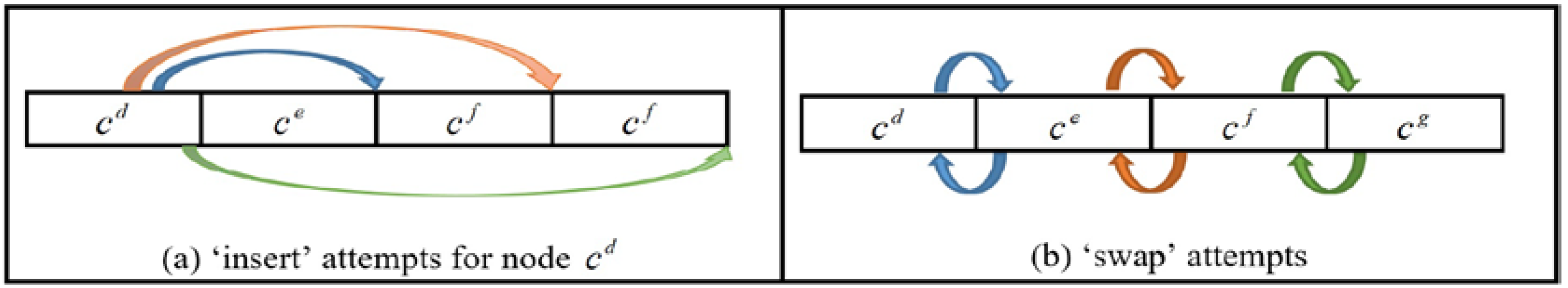
The first layer local search is applied on the all “feasible” particles, for which routes could be successfully made by Algorithm 1, in the population in every iteration of PSO. We apply Intra-Route Local Search (Intra-RLS) followed by Inter-Route Local Search (Inter-RLS) to exploit the neighborhood of a particle to look for any better solution before moving to another position in the solution space in the next iteration of PSO. In the Intra-RLS, we apply “swap” and “insertion” strategies on every route constructed for the particle at hand. In the “swap” stage, we interchange the neighboring nodes in a route if it minimizes the total distance of the route. For “insertion”, we pick a node, and try to insert it in other possible positions in the route if it decreases the total distance of the route. After all the nodes have been checked, the move with the best gain can be executed. We apply “insertion” operation using the nodes one after another onward from the starting of a route until any node succeeds to move to another position. We do not perform all possible exploration here to keep the complexity of the algorithm tolerable. Moreover, there remains a possibility for the proposed second layer of local search to explore more “insertion” options on the potential solutions that are selected in the “pool” (please see Section 3.3.2 for details).
A portrayal of the attempts made by the “insert” and “swap” operations on a route (cd, ce, cf and cg) are illustrated in Figure 3.
The Inter-RLS strategy also applies the similar “insertion” and “swap” operations, but between two different routes. Inter-RLS is portrayed in Figure 4. The arrows show the “insert” options to be tried by node 1, from which the best one is to be performed if it decreases the total distance of the two concerned routes.
It is worth mentioning here that the “insertion” operation is not allowed to remove all the nodes of a route into another route thus the required number of vehicles will be constant throughout the program run.
3.3.2. The Second Layer Local Search
The operations of the second layer of local search are similar to those in the first layer. As mentioned earlier, this layer of local search is applied on a pool of the global best solutions attained in different iterations the PSO algorithm. This is an approach to exploit the best-found solution more deeply as some of them might be very close to the optimal solution.
To limit the growth of the pool, we refine it by deleting some of the solutions in the pool according to Algorithm 2 at every iteration. It keeps the best solution in the pool. It also keeps the solutions that were updated by the local search in the previous iteration for the hope that they may be further updated in the upcoming iterations to attain better solutions. The solution that neither is the best in the pool nor was updated in the previous iteration is deleted from the pool because it can no longer be updated by the proposed local search.
| Algorithm 2. Refining the pool of solutions |
| Input P: a pool of global best solutions Output P’: The refined pool of solutions Procedure 1. for each solution s in P do 2. if s is the best solution in P then 3. add s to P’ 4. else if s was updated in the previous iteration then 5. add s to P’ 6. end if 7. end for |
4. Computational Result Analysis
We have implemented the proposed bilayer local search enhanced particle swarm optimization (BLS-PSO) in MATLAB R2017a environment on a personal computer with a processor Intel® Pentium® Dual-Core CPU T4300 @ 2.10 GHz (only single core is used), memory (RAM) of 2.0 GB, and Windows 10 Education version.
We have considered seven sets of capacitated vehicle routing benchmark problems of the well-known CVRPLIB problem set which are also used for the verification of many PSO-based proposals [41], can be downloaded from http://vrp.atd-lab.inf.puc-rio.br/index.php/en/. The benchmark problem sets are called Set A, Set B, Set P [55], Set E, Set F, Set M [56] and Set CMT [57]. The problems in the Sets A, B, E, F, M and P specify only capacity constraints for the vehicles, but not any constraint on the distance travelled by a vehicle. Total number of customers varies from 15 to 199 in these sets, and locations of the customers, except Sets B and M, are generated in random scattered manner or, following semi-clustered fashion [52]. The problems in Set B and M are generated in a clustered layout [52]. Though some researchers [41] pick a subset of the 92 problems to demonstrate the performances of their proposed algorithms, we have considered all the problems to show the real portrayal of the performance of our proposed BLS-PSO on a variety of problems.
Chen et al. [41] considered all the 14 problems of the CMT problem set. CMT1, CMT2, CMT3, CMT4, CMT5, CMT11 and CMT12 consider only the capacity constraint for the vehicles whereas CMT6, CMT7, CMT8, CMT9, CMT10, CMT13 and CMT14 have additional restrictions on the maximum travelling distance of a vehicle. In CMT, problem sets include 50 to 199 customers, whose locations are randomly scattered in CMT1 to CMT10 problem sets while clustered locations are set in CMT11 to CMT14.
4.1. Setting the Parameters
A fundamental characteristic of metaheuristic algorithms is that their performance is greatly parameter value intensive. Quality of solution obtained and required computational time to solve a problem critically depend on the parameter sets. As optimizing the parameter sets for any metaheuristic algorithm is itself an optimization problem, we have run all the problems for different parameter sets and selected the best result achieving parameter set for this article. In the parameter set optimization step, there are several parameter values to be decided such as population size or the number of particles PSParticle, maximum number of iterations, T, constants in PSO equation k1, k2 and k3, termination criteria and so on. We have performed a set of experiments to fix the parameter sets to obtain the best out of the proposed bilayer local search-based particle swarm optimization (BLS-PSO) algorithm. The experimental designed setup for the experiments are portrayed in Table 3.
The termination criteria used in our approach is that the program run until the maximum number of iterations, T. For BLS-PSO, we have reported the average of the performances of 20 runs for the best combination of k2 and k3 for a problem, unless specified otherwise.
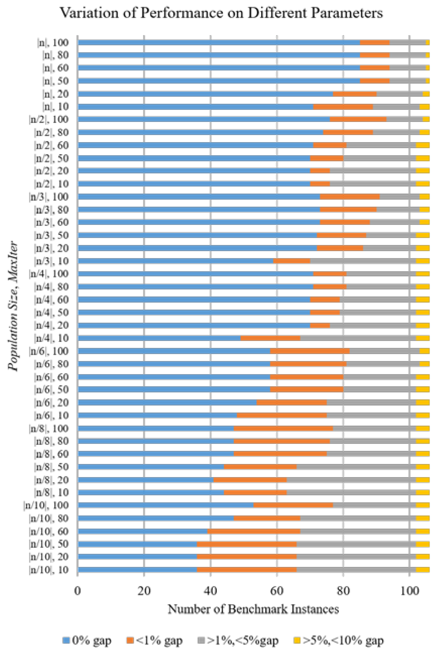
The experiments show that performance of the proposed algorithm get improved with increasing both population size, PSParticle and maximum number of iteration, T portrayed in Figure 5. It is observed that even if the PSParticle and T is increased up to certain limit, the proposed algorithm can find results equal to best known solutions at most for 85 benchmark instances. When the setting PSParticle is equal to the number of nodes in respective problem statement and T is 50 or more it can find the results equal to the best-known solutions for maximum 85 benchmark problems. Not finding the outputs equal to the best-known solutions for the remaining problem instances are likely due to having two reasons either the small population size or the number of maximum iteration which is set as low as 100. However, as an approximate algorithm is expected to find a near optimal or, a “good” solution within a small computational time, we have chosen the PSParticle as equal to n and T as 50.
For setting the value of k2 and k3, we have run the program again with the parameter setting of PSParticle and T as mentioned above. In these experimental setups, for a particular k2 we have run the program for all k3 values. For any setup, the number of best known results found is marked on the pie chart in Figure 6. Close observation portrays that there is no significant converging point to fix the value of k2 and k3 to obtain the best performance of the proposed algorithm. However, the computational time required for one complete run of the proposed algorithm for an instance is not significant. Thus, experiments for all the combinations of k2 and k3 for each instance is performed thoroughly and the best result achieved by the proposed BLS-PSO is reported in later subsections.
4.2. Result Analysis
Table 4, Table 5, Table 6, Table 7, Table 8, Table 9 and Table 10 present the computational results obtained by BLS-PSO for several benchmark problem sets, where m represents the required number of vehicles for the corresponding problem instance, Cost reports the best fitness obtained by an algorithm along with the corresponding gap in percentage, representing the quality of a solution, calculated as
where CostBLS-PSO is the best solution obtained by the proposed method and BKS is the best-known solution for the same instance reported in the literature. AvgT is average of CPU times required by 20 individual runs for particular k2 and k3 value to reach the corresponding best solution. As we have mentioned, k2 and k3 values are not same for all the problems, we have mentioned the specific k2 and k3 values for each instance. Although the values of k2 and k3 tabulated in the tables are not mandatorily the only combination to find the results rather there may many other combinations giving the same results. We have mentioned only one combination here for the consistency in the presentation of the tables.
The proposed BLS-PSO algorithm has reached the best-known solutions for 84 instances out of the 106 Euclidean distance-based benchmark instances used in our experiments. BLS-PSO has an average gap of 0.07%, 0.14%, 0.31%, 0.26%, 3.45%, 0.2% and 0.64% to solve instances in Sets A, B, E, F, M, P and CMT, respectively. It requires an average CPU Time of 5.5 s, 6.13 s, 11.51 s, 25.59 s, 68.69 s, 4.72 s and 13.33 s to solve instances in Set A, B, E, F, M, P and CMT, respectively. Thus, BLS-PSO has been found to obtain the results equal to the best-known results for most of the existing benchmark problems within short computational time.
BLS-PSO has not met the best-known results for some instances. The main reason behind this may be the small population size or the lower value of the maximum number of iterations. Increasing them are expected to attain better solutions.
4.3. Comparative Performance of PSO-Based Approaches
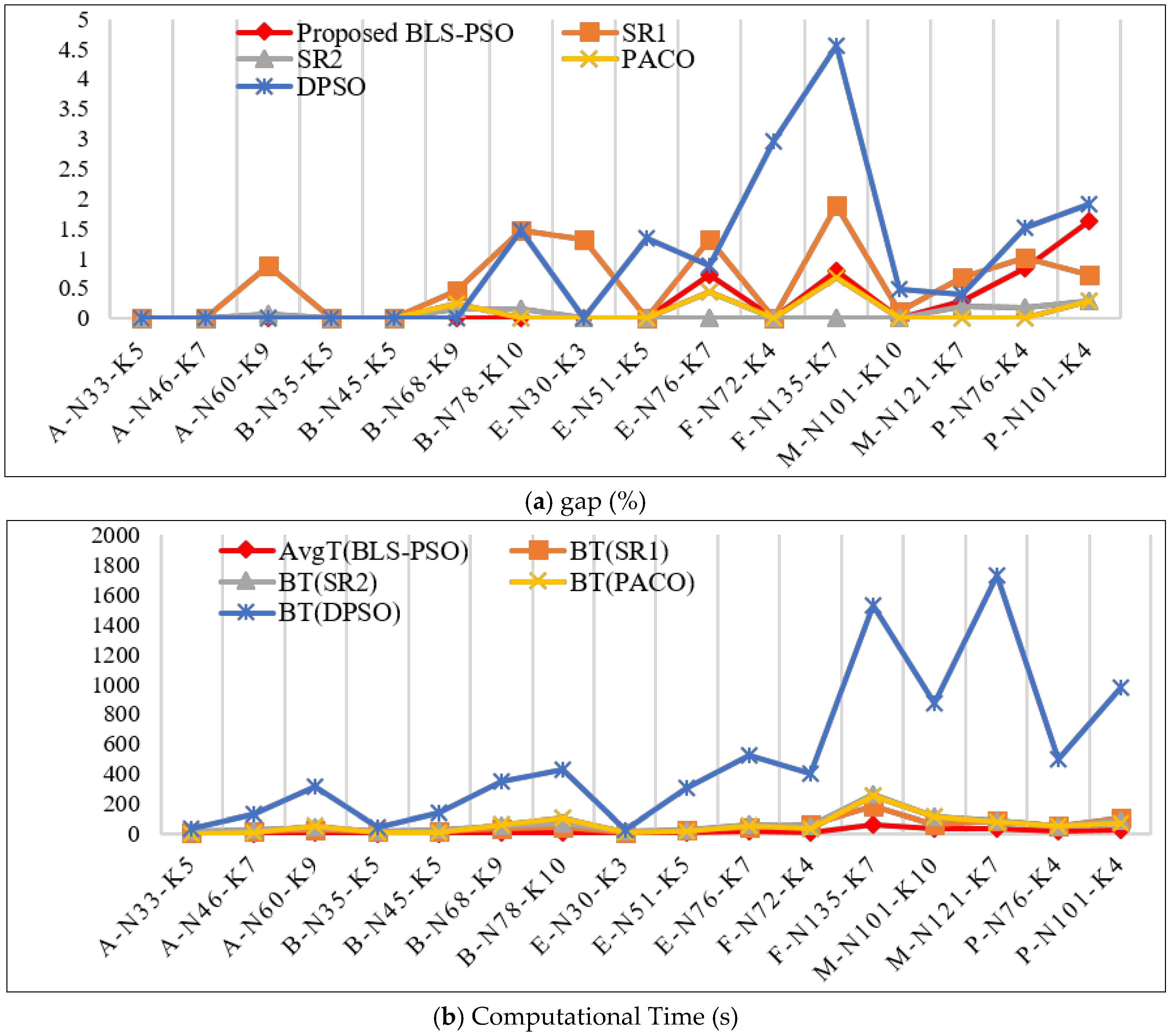
To portray the comparison of the performance of our proposed algorithm with other PSO-based algorithms in the literature, we have taken the same instances used by other researchers [41,44,47,52]. Table 11 contains the results for 16 instances from the Sets A, B, E, F, M and P, and Table 12 lists results for all the 14 instances of Set CMT. Here, PSO-based algorithms DPSO [41], SR1, SR2 [44,46] and PSCO [52] are compared with proposed BLS-PSO. Here, Cost is the result obtained by respective algorithms and a value is in boldface font when it is equal to the best-known result reported in the literature. The superscript “a” indicates that the cost is inferior to what is achieved by the proposed BLS-PSO. BT refers to the computational time in seconds to reach the corresponding result. For the proposed algorithm, we have reported the AvgT as mentioned earlier. As mentioned above there are no convergence of solution for specific k2 and k3 value, we have mentioned AvgCost as the average of all the solutions obtained by BLS-PSO for different k2 and k3. The deviation of the AvgCost with the best-known solutions is mentioned as SD in Table 11. It is evident that even the average time taken by the proposed method is far better, let alone the shortest time, than the shortest time of other approaches for each of the problem instances under consideration.
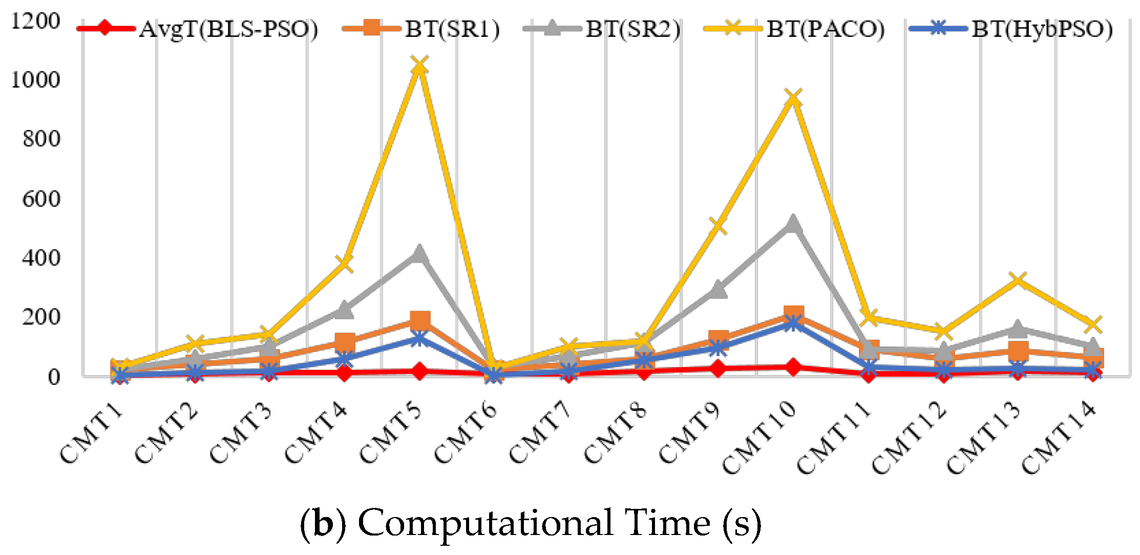
The overall results are also graphically represented in Figure 7 to show the comparative performances more comprehensively. The negative gap in Figure 7a corresponds to the problem instance, for which the BLS-PSO has obtained a new optimal result. Figure 7b demonstrates that time consumed by BLS-PSO is significantly less than the other approaches, where the plot is almost touching the horizontal axis for all the instances.
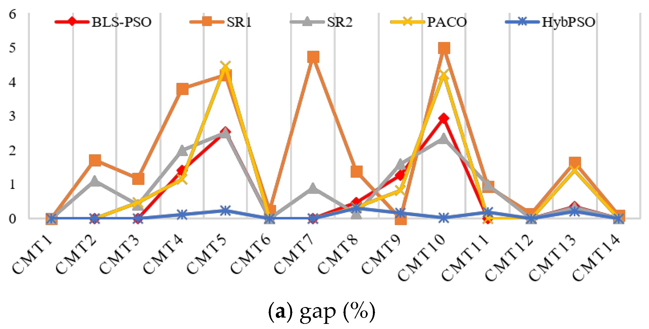
Table 12 portrays the comparison of performance in handling CMT problem set instances. Here we have compared SR1, SR2 [44,46], HybPSO [47] and PSCO [52] with the proposed BLS-PSO.
Figure 8 shows clearer comparative graphical representations of the performances of the PSO-based algorithms dealing instances in Set CMT. Here, BLS-PSO has obtained results equal to the best known results with an average gap of 0.64% whereas SR1, SR2, PACO and HybPSO have gap of 1.788%, 0.874%, 0.913% and 0.084% respectively. However, the average of the reported CPU times required by BLS-PSO is only 13.33 s to solve the instances in Set CMT whereas the average of the best times required by SR1, SR2, PACO and HybPSO are 84.1 s, 163.1 s, 302.58 s and 48.13 s, respectively. Hence, although the gap values obtained by the proposed algorithm are higher than the other methods for some instances, BLS-PSO is found to reach to the best known results for most of the cases in significantly lower computational times as compared to the other algorithms. This advocates for its efficiency.
5. Conclusions
In this article, we have proposed a bilayer local search-based Particle Swarm Optimization (BLS-PSO) incorporated with a simple chromosome structure to apply PSO operations easily. We have also proposed a decoding technique that depends on the number of vehicles needed to serve the customers which is specified in the problem statement of benchmark instances considered in this article, and then build the routes in a comprehensible solution on which we apply the proposed local searches. The first layer of the proposed bilayer local search approach searches the neighborhood of all particles to find better solution whereas the second layer is applied on the pool of the best particle of different generations. The first layer is important for exploring the neighborhoods of the particles before modifying the chromosomes by PSO operations, and the second layer gives more chances to the best selected particles to exploit more of their neighborhoods. Such a contribution helps the search strategy to obtain optimal or near optimal solutions with the expense of very short computational time, which is also evident from the experimental results obtained by applying the method on different benchmark problem sets.
The proposed decoding method can also be easily integrated with other population-based metaheuristics to solve CVRP where a solution is encoded as a permutation of customer nodes. The bilayer search strategy may also enhance the performances of other nature-inspired searching strategies. Moreover, introduction of a probabilistic approach to the decoding algorithm may also contribute to generate different potential solutions. The estimation procedure of the required number of vehicles may also be enhanced by using a stochastic technique other than taking as input from the problem statement to solve generalized vehicle routing problems. We leave all these possibilities to be investigated in our future endeavors.
Acknowledgments
This work was supported by Hankuk University of Foreign Studies Research Fund.
Author Contributions
A. K. M. Foysal Ahmed and Ji Ung Sun conceived and designed the experiments; A. K. M. Foysal Ahmed performed the experiments; A. K. M. Foysal Ahmed and Ji Ung Sun analyzed the data; A. K. M. Foysal Ahmed contributed analysis tools; A. K. M. Foysal Ahmed wrote the paper.
Conflicts of Interest
The authors declare no conflict of interest.
References
- Ćirović, G.; Pamučar, D.; Božanić, D. Green logistic vehicle routing problem: Routing light delivery vehicles in urban areas using a neuro-fuzzy model. Expert Syst. Appl. 2014, 41, 4245–4258. [Google Scholar] [CrossRef]
- Dell’Amico, M.; Righini, G.; Salani, M. A branch-and-price approach to the vehicle routing problem with simultaneous distribution and collection. Transp. Sci. 2006, 40, 235–247. [Google Scholar] [CrossRef]
- Erdoğan, S.; Miller-Hooks, E. A green vehicle routing problem. Transp. Res. Part E 2012, 48, 100–114. [Google Scholar] [CrossRef]
- Lei, H.; Laporte, G.; Guo, B. The capacitated vehicle routing problem with stochastic demands and time windows. Comput. Oper. Res. 2011, 38, 1775–1783. [Google Scholar] [CrossRef]
- Xiao, Y.; Zhao, Q.; Kaku, I.; Xu, Y. Development of a fuel consumption optimization model for the capacitated vehicle routing problem. Comput. Oper. Res. 2012, 39, 1419–1431. [Google Scholar] [CrossRef]
- Dantzig, G.B.; Ramser, J.H. The truck dispatching problem. Manag. Sci. 1959, 6, 80–91. [Google Scholar] [CrossRef]
- Lenstra, J.K.; Kan, A.H.G. Complexity of vehicle routing and scheduling problems. Networks 1981, 11, 221–227. [Google Scholar] [CrossRef]
- Christofides, N.; Mingozzi, A.; Toth, P. Exact algorithms for the vehicle routing problem, based on spanning tree and shortest path relaxations. Math. Program. 1981, 20, 255–282. [Google Scholar] [CrossRef]
- Clarke, G.; Wright, J.W. Scheduling of vehicles from a central depot to a number of delivery points. Oper. Res. 1964, 12, 568–581. [Google Scholar] [CrossRef]
- Gaskell, T.J. Bases for vehicle fleet scheduling. J. Oper. Res. Soc. 1967, 18, 281–295. [Google Scholar] [CrossRef]
- Mole, R.H.; Jameson, S.R. A sequential route-building algorithm employing a generalised savings criterion. J. Oper. Res. Soc. 1976, 27, 503–511. [Google Scholar] [CrossRef]
- Paessens, H. The savings algorithm for the vehicle routing problem. Eur. J. Oper. Res. 1988, 34, 336–344. [Google Scholar] [CrossRef]
- Fisher, M.L.; Jaikumar, R. A generalized assignment heuristic for vehicle routing. Networks 1981, 11, 109–124. [Google Scholar] [CrossRef]
- Gillett, B.E.; Miller, L.R. A heuristic algorithm for the vehicle-dispatch problem. Oper. Res. 1974, 22, 340–349. [Google Scholar] [CrossRef]
- Beasley, J.E. Route first—Cluster second methods for vehicle routing. Omega 1983, 11, 403–408. [Google Scholar] [CrossRef]
- Goldberg, D.E. Genetic Algorithms in Search, Optimization, and Machine Learning. Mach. Learn. 1988, 3, 95–99. [Google Scholar] [CrossRef]
- Berger, J.; Barkaoui, M. A hybrid genetic algorithm for the capacitated vehicle routing problem. In Proceedings of the Conference on Genetic and Evolutionary Computation, Chicago, IL, USA, 12–16 July 2003; Springer: Berlin/Heidelberg, Germany, 2003; pp. 646–656. [Google Scholar]
- Glover, F. Tabu search—Part I. ORSA J. Comput. 1989, 1, 190–206. [Google Scholar] [CrossRef]
- Glover, F. Tabu search—Part II. ORSA J. Comput. 1990, 2, 4–32. [Google Scholar] [CrossRef]
- Toth, P.; Vigo, D. The granular tabu search and its application to the vehicle-routing problem. Informs J. Comput. 2003, 15, 333–346. [Google Scholar] [CrossRef]
- Kirkpatrick, S.C.; Gelatt, D.; Vecchi, M.P. Optimization by simulated annealing. Science 1983, 220, 671–680. [Google Scholar] [CrossRef] [PubMed]
- Lin, S.W.; Lee, Z.J.; Ying, K.C.; Lee, C.Y. Applying hybrid meta-heuristics for capacitated vehicle routing problem. Expert Syst. Appl. 2009, 36, 1505–1512. [Google Scholar] [CrossRef]
- Baker, B.M.; Ayechew, M.A. A genetic algorithm for the vehicle routing problem. Comput. Oper. Res. 2003, 30, 787–800. [Google Scholar] [CrossRef]
- Carwalo, T.; Thankappan, J.; Patil, V. Capacitated vehicle routing problem. In Proceedings of the 2nd International IEEE Conference on Communication Systems, Computing and IT Applications (CSCITA), Mumbai, India, 7–8 April 2017; pp. 17–21. [Google Scholar]
- Hertz, A.; Laporte, G.; Mittaz, M. A tabu search heuristic for the capacitated arc routing problem. Oper. Res. 2000, 48, 129–135. [Google Scholar] [CrossRef]
- Teymourian, E.; Kayvanfar, V.; Komaki, G.M.; Zandieh, M. Enhanced intelligent water drops and cuckoo search algorithms for solving the capacitated vehicle routing problem. Inf. Sci. 2016, 334, 354–378. [Google Scholar] [CrossRef]
- Yu, B.; Yang, Z.Z.; Yao, B. An improved ant colony optimization for vehicle routing problem. Eur. J. Oper. Res. 2009, 196, 171–176. [Google Scholar] [CrossRef]
- Blum, C.; Li, X. Swarm Intelligence. In Swarm Intelligence in Optimization; Blum, C., Merkle, D., Eds.; Springer: Berlin/Heidelberg, Germany, 2008; pp. 43–85. [Google Scholar]
- Hu, X.; Eberhart, R.C.; Shi, Y. Swarm intelligence for permutation optimization: A case study of n-queens problem. In Proceedings of the IEEE Swarm Intelligence Symposium, Indianapolis, IN, USA, 26 April 2003; pp. 243–246. [Google Scholar]
- Marinakis, Y.; Marinaki, M. A hybrid genetic–Particle Swarm Optimization Algorithm for the vehicle routing problem. Expert Syst. Appl. 2010, 37, 1446–1455. [Google Scholar] [CrossRef]
- Chen, P.; Huang, H.K.; Dong, X.Y. Iterated variable neighborhood descent algorithm for the capacitated vehicle routing problem. Expert Syst. Appl. 2010, 37, 1620–1627. [Google Scholar] [CrossRef]
- Kytöjoki, J.; Nuortio, T.; Bräysy, O.; Gendreau, M. An efficient variable neighborhood search heuristic for very large scale vehicle routing problems. Comput. Oper. Res. 2007, 34, 2743–2757. [Google Scholar] [CrossRef]
- Mazzeo, S.; Loiseau, I. An ant colony algorithm for the capacitated vehicle routing. Electron. Notes Discret. Math. 2004, 18, 181–186. [Google Scholar] [CrossRef]
- Nazif, H.; Lee, L.S. Optimised crossover genetic algorithm for capacitated vehicle routing problem. Appl. Math. Model. 2012, 36, 2110–2117. [Google Scholar] [CrossRef]
- Ngueveu, S.U.; Prins, C.; Calvo, R.W. An effective memetic algorithm for the cumulative capacitated vehicle routing problem. Comput. Oper. Res. 2010, 37, 1877–1885. [Google Scholar] [CrossRef]
- Szeto, W.Y.; Wu, Y.; Ho, S.C. An artificial bee colony algorithm for the capacitated vehicle routing problem. Eur. J. Oper. Res. 2011, 215, 126–135. [Google Scholar] [CrossRef] [Green Version]
- Zhou, Y.; Luo, Q.; Xie, J.; Zheng, H. A hybrid bat algorithm with path relinking for the capacitated vehicle routing problem. In Metaheuristics and Optimization in Civil Engineering; Springer: Cham, Switzerland, 2016; Volume 7, pp. 255–276. [Google Scholar]
- Banks, A.; Vincent, J.; Anyakoha, C. A review of particle swarm optimization. Part I: Background and development. Nat. Comput. 2007, 6, 467–484. [Google Scholar] [CrossRef]
- Banks, A.; Vincent, J.; Anyakoha, C. A review of particle swarm optimization. Part II: Hybridisation, combinatorial, multicriteria and constrained optimization, and indicative applications. Nat. Comput. 2008, 7, 109–124. [Google Scholar] [CrossRef]
- Eberhart, R.C.; Kennedy, J. Particle swarm optimization. In Proceedings of the IEEE International Conference on Neural Network, Perth, Australia, 27 November–1 December 1995; pp. 1942–1948. [Google Scholar]
- Chen, A.L.; Yang, G.K.; Wu, Z.M. Hybrid discrete particle swarm optimization algorithm for capacitated vehicle routing problem. J. Zhejiang Univ.-Sci. A 2006, 7, 607–614. [Google Scholar] [CrossRef]
- Yang, S.; Wang, M. A quantum particle swarm optimization. In Proceedings of the Congress on Evolutionary Computation, Portland, OR, USA, 19–23 June 2004; pp. 320–324. [Google Scholar]
- Kao, Y.; Chen, M. A Hybrid PSO Algorithm for the CVRP Problem. In Proceedings of the IJCCI (ECTA-FCTA), Paris, France, 24–26 October 2011; pp. 539–543. [Google Scholar]
- Ai, T.J.; Kachitvichyanukul, V. Particle swarm optimization and two solution representations for solving the capacitated vehicle routing problem. Comput. Ind. Eng. 2009, 56, 380–387. [Google Scholar] [CrossRef]
- Pongchairerks, C.; Kachitvichyanukul, V. A non-homogenous particle swarm optimization with multiple social structures. In Proceedings of the International Conference on Simulation and Modeling, Nakorn Pathom, Thailand, 17–19 January 2005; pp. 132–136. [Google Scholar]
- Ai, T.J.; Kachitvichyanukul, V. A particle swarm optimization for the capacitated vehicle routing problem. Int. J. Logist. SCM Syst. 2007, 2, 50–55. [Google Scholar]
- Marinakis, Y.; Marinaki, M.; Dounias, G. A hybrid particle swarm optimization algorithm for the vehicle routing problem. Eng. Appl. Artif. Intell. 2010, 23, 463–472. [Google Scholar] [CrossRef]
- Marinakis, Y.; Migdalad, A.; Pardalos, P.M. Multiple phase neighborhood Search–GRASP based on Lagrangean relaxation, random backtracking Lin–Kernighan and path relinking for the TSP. J. Comb. Optim. 2009, 17, 134–156. [Google Scholar] [CrossRef]
- Marinakis, Y.; Migdalad, A.; Pardalos, P.M. Expanding neighborhood GRASP for the traveling salesman problem. Comput. Optim. Appl. 2005, 32, 231–257. [Google Scholar] [CrossRef]
- Marinakis, Y.; Migdalad, A.; Pardalos, P.M. A Hybrid Genetic–GRASP Algorithm Using Lagrangean Relaxation for the Traveling Salesman Problem. J. Comb. Optim. 2005, 10, 311–326. [Google Scholar] [CrossRef]
- Glover, F.; Laguna, M.; Marti, R. Scatter Search and Path Relinking: Advances and Applications. In Handbook of Metaheuristics; Springer: New York, NY, USA, 2003; pp. 1–35. [Google Scholar]
- Kao, Y.; Chen, M.H.; Huang, Y.T. A hybrid algorithm based on ACO and PSO for capacitated vehicle routing problems. Math. Probl. Eng. 2012, 2012, 1–17. [Google Scholar] [CrossRef]
- Shi, Y.; Eberhart, R.C. A modified particle swarm optimizer. In Proceedings of the IEEE International Conference on Evolutionary Computation, Anchorage, AK, USA, 4–9 May 1998; pp. 69–73. [Google Scholar]
- Wang, K.P.; Huang, L.; Zhou, C.G.; Pang, W. Particle swarm optimization for traveling salesman problem. In Proceedings of the IEEE International Conference on Machine Learning and Cybernetics, Xi’an, China, 5 November 2003; pp. 1583–1585. [Google Scholar]
- Augerat, P.; Belenguer, J.; Benavent, E.; Corberán, A.; Naddef, D.; Rinaldi, G. Computational Results with a Branch and Cut Code for the Capacitated Vehicle Routing Problem; Technical report 949-M; Université Joseph Fourier: Grenoble, France, 1995. [Google Scholar]
- Christofides, N.; Mingozzi, A.; Toth, P. An algorithm for the vehicle-dispatching problem. Oper. Res. Q. 1969, 20, 309–318. [Google Scholar] [CrossRef]
- Christofides, N.; Mingozzi, A.; Toth, P. The Vehicle Routing Problem. In Combinatorial Optimization; Wiley Interscience: Hoboken, NJ, USA, 1979; pp. 315–338. [Google Scholar]
- Akhand, M.A.H.; Akter, S.; Rashid, M.A.; Yaakob, S.B. Velocity Tentative PSO: An Optimal Velocity Implementation based Particle Swarm Optimization to Solve Traveling Salesman Problem. Prod. Plan. Control 2015, 42, 221–232. [Google Scholar]
Figure 1.
A portrayal of capacitated vehicle routing problem.

Figure 2.
Flowchart diagram of the proposed BLS-PSO.
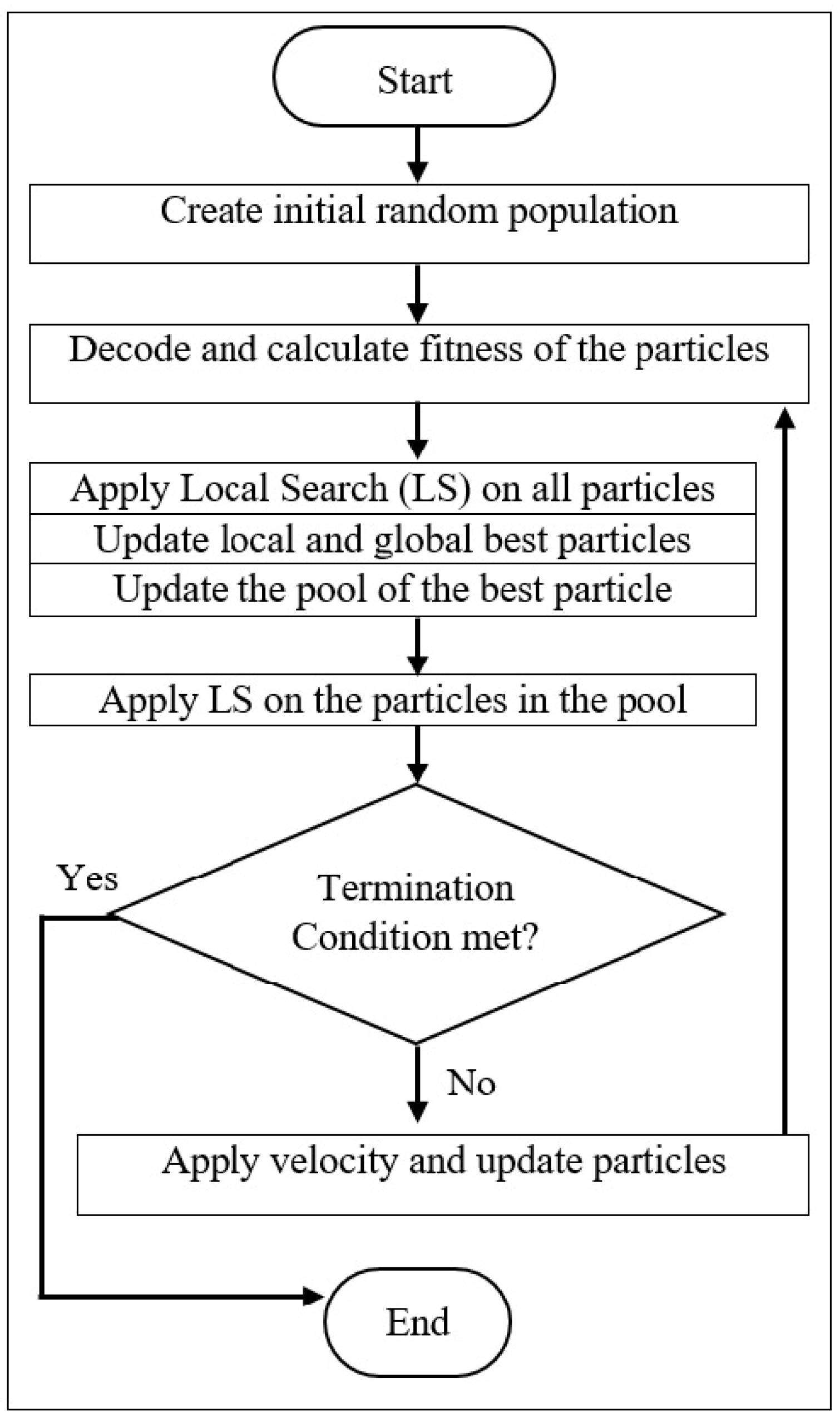
Figure 3.
An illustration of Intra-Route Local Search. (a) ‘insert’ attempts for node cd; (b) ’swap’ attempts.
Figure 3.
An illustration of Intra-Route Local Search. (a) ‘insert’ attempts for node cd; (b) ’swap’ attempts.

Figure 4.
An illustration of Inter-Route Local Search.
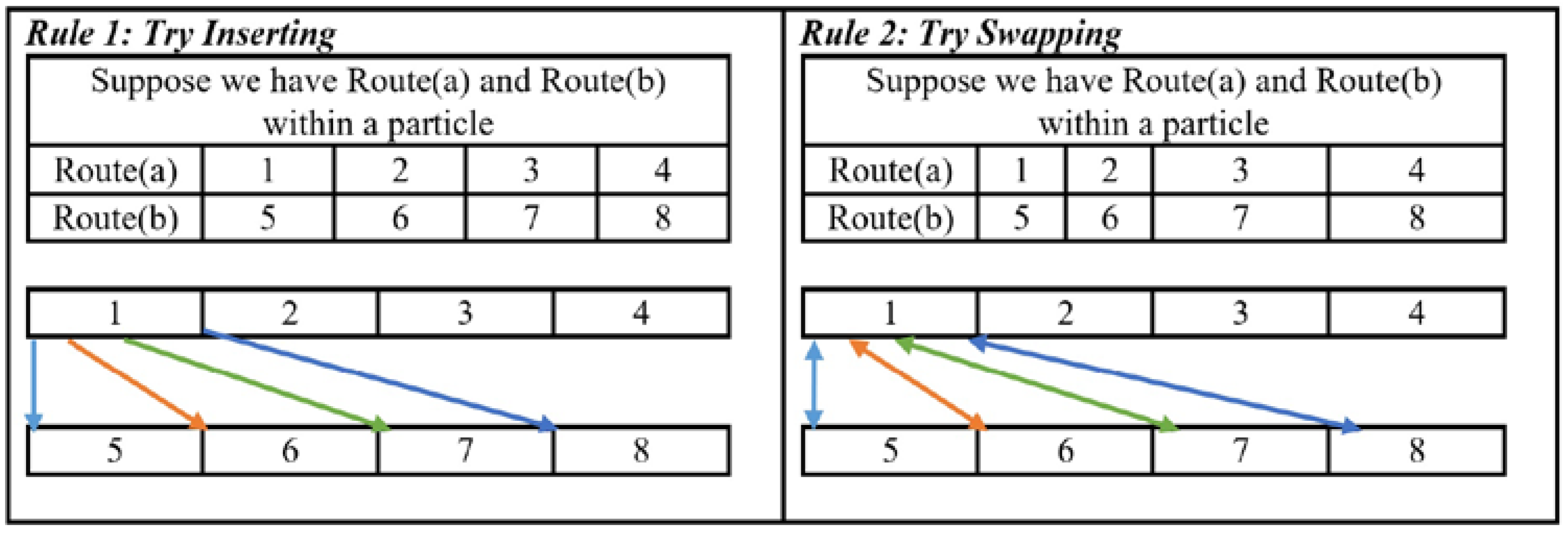
Figure 5.
Variation in convergence of BLS-PSO depending on different PSParticle & T.

Figure 6.
Scattered variation of convergence of the proposed BLS-PSO depending on different values of parameters k2 and k3.
Figure 6.
Scattered variation of convergence of the proposed BLS-PSO depending on different values of parameters k2 and k3.
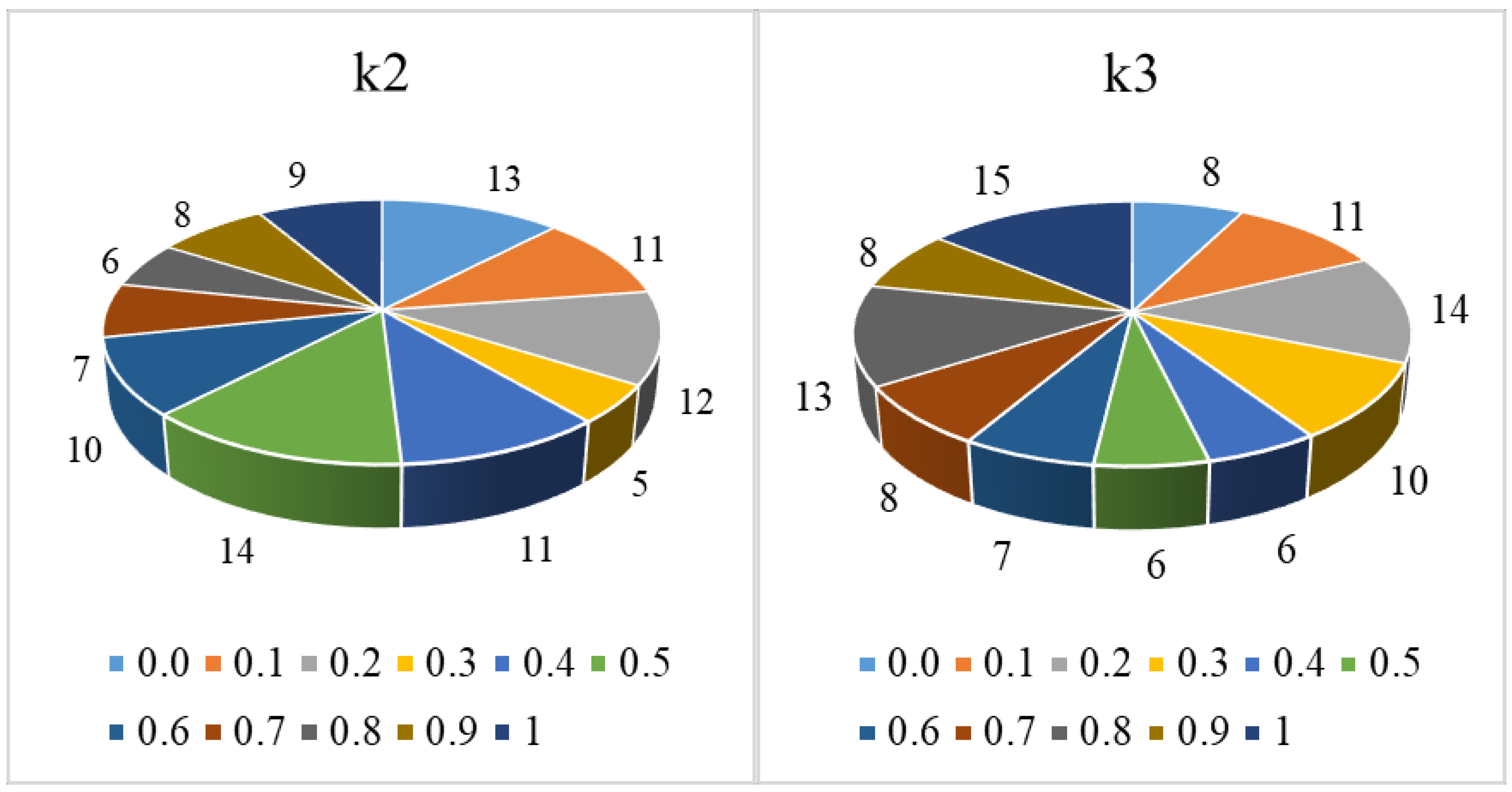
Figure 7.
Performances of different algorithms in solving selective instances. (a) gap (%); (b) Computational Time (s).
Figure 7.
Performances of different algorithms in solving selective instances. (a) gap (%); (b) Computational Time (s).

Figure 8.
Performances of different algorithms in solving Set CMT instances. (a) gap (%); (b) Computational Time (s).
Figure 8.
Performances of different algorithms in solving Set CMT instances. (a) gap (%); (b) Computational Time (s).


Table 1.
Related notations and variables for CVRP formulation defined in this article.
| N | Total number of nodes |
| m | Total number of required vehicles |
| Cost to visit node ck from node cj | |
| Service time required when a vehicle visits node i (for the depot, ) | |
| Q | Maximum capacity of a vehicle |
| TT | Maximum distance of a vehicle can travel to |
| di | Demand of a customer to be served by a vehicle |
| Z | Customer set served by a vehicle; |Z| is the number of customers served by a vehicle |
| Binary decision variable set to 1 if vehicle v serves node k after serving node j, or 0 otherwise |
Table 2.
Hub ID, Customer IDs and associated demands in example problem instance.
| Hub ID | Customer IDs | ||||||||||
|---|---|---|---|---|---|---|---|---|---|---|---|
| IDs | 1 | 2 | 3 | 4 | 5 | 6 | 7 | 8 | 9 | 10 | 11 |
| Demands | 0 | 17 | 8 | 16 | 28 | 13 | 8 | 23 | 7 | 6 | 15 |
Table 3.
Different values of parameters used in experimental setup.
| PSParticle | T | k2 | k3 |
|---|---|---|---|
| {|n/10|, |n/8|, |n/6|, |n/4|, |n/3|, |n/2|, |n|} | {10, 20, 50, 60, 80, 100} | {between 0 and 1 (with 0.1 interval)} | {between 0 and 1 (with 0.1 interval)} |
Table 4.
Performance of BLS-PSO in solving the benchmark problems in Set A.
| Problems | BKS | CostBLS-PSO | gap | AvgT | k2 | k3 |
|---|---|---|---|---|---|---|
| A-n32-k5 | 784 | 784 | 0.00 | 0.15 | 0.1 | 0.1 |
| A-n33-k5 | 661 | 661 | 0.00 | 0.15 | 0.4 | 0.5 |
| A-n33-k6 | 742 | 742 | 0.00 | 0.43 | 0.4 | 0.0 |
| A-n34-k5 | 778 | 778 | 0.00 | 0.8 | 0.5 | 0.8 |
| A-n36-k5 | 799 | 799 | 0.00 | 0.76 | 0.0 | 0.8 |
| A-n37-k5 | 669 | 669 | 0.00 | 0.92 | 0.8 | 1.0 |
| A-n37-k6 | 949 | 949 | 0.00 | 0.64 | 0.5 | 0.2 |
| A-n38-k5 | 730 | 730 | 0.00 | 0.69 | 1.0 | 0.8 |
| A-n39-k5 | 822 | 822 | 0.00 | 1.07 | 0.5 | 0.3 |
| A-n39-k6 | 831 | 831 | 0.00 | 1.15 | 0.4 | 0.7 |
| A-n44-k6 | 937 | 937 | 0.00 | 1.03 | 0.3 | 0.0 |
| A-n45-k6 | 944 | 944 | 0.00 | 1.76 | 0.0 | 0.2 |
| A-n45-k7 | 1146 | 1146 | 0.00 | 1.31 | 0.5 | 0.0 |
| A-n46-k7 | 914 | 914 | 0.00 | 1.29 | 0.6 | 0.3 |
| A-n48-k7 | 1073 | 1073 | 0.00 | 1.45 | 0.9 | 0.1 |
| A-n53-k7 | 1010 | 1010 | 0.00 | 2.54 | 0.9 | 1.0 |
| A-n54-k7 | 1167 | 1167 | 0.00 | 7.61 | 0.2 | 0.5 |
| A-n55-k9 | 1073 | 1073 | 0.00 | 8.47 | 0.5 | 0.4 |
| A-n60-k9 | 1354 | 1354 | 0.00 | 8.78 | 0.6 | 0.2 |
| A-n61-k9 | 1034 | 1034 | 0.00 | 7.98 | 0.7 | 1.0 |
| A-n62-k8 | 1288 | 1296 | 0.62 | 9.53 | 0.7 | 0.4 |
| A-n63-k9 | 1616 | 1616 | 0.00 | 9.22 | 0.9 | 0.3 |
| A-n63-k10 | 1314 | 1314 | 0.00 | 10.14 | 0.8 | 1.0 |
| A-n64-k9 | 1401 | 1415 | 1.00 | 18.86 | 0.5 | 0.6 |
| A-n65-k9 | 1174 | 1174 | 0.00 | 16.5 | 0.2 | 0.8 |
| A-n69-k9 | 1159 | 1159 | 0.00 | 18.41 | 0.6 | 0.6 |
| A-n80-k10 | 1763 | 1766 | 0.17 | 16.75 | 0.2 | 1.0 |
| Average | 0.07 | 5.5 | -- | -- | ||
Table 5.
Performance of BLS-PSO in solving the benchmark problems in Set B.
| Problems | BKS | CostBLS-PSO | gap | AvgT | k2 | k3 |
|---|---|---|---|---|---|---|
| B-n31-k5 | 672 | 672 | 0.00 | 2.07 | 0.5 | 0.5 |
| B-n34-k5 | 788 | 788 | 0.00 | 2.42 | 0.1 | 0.9 |
| B-n35-k5 | 955 | 955 | 0.00 | 1.12 | 0.6 | 0.8 |
| B-n38-k6 | 805 | 805 | 0.00 | 3.01 | 0.8 | 0.9 |
| B-n39-k5 | 549 | 549 | 0.00 | 3.59 | 0.0 | 0.3 |
| B-n41-k6 | 829 | 829 | 0.00 | 3.93 | 0.2 | 0.3 |
| B-n43-k6 | 742 | 742 | 0.00 | 2.55 | 0.7 | 0.1 |
| B-n44-k7 | 909 | 909 | 0.00 | 3.16 | 0.0 | 0.3 |
| B-n45-k5 | 751 | 751 | 0.00 | 2.04 | 0.8 | 0.2 |
| B-n45-k6 | 672 | 672 | 0.00 | 4.95 | 0.5 | 0.5 |
| B-n50-k7 | 741 | 741 | 0.00 | 5.45 | 0.3 | 0.2 |
| B-n50-k8 | 1312 | 1312 | 0.00 | 5.53 | 0.0 | 0.0 |
| B-n51-k7 | 1032 | 1032 | 0.00 | 5.39 | 0.2 | 0.0 |
| B-n52-k7 | 747 | 747 | 0.00 | 6.18 | 0.1 | 0.6 |
| B-n56-k7 | 707 | 707 | 0.00 | 7.31 | 0.2 | 0.2 |
| B-n57-k7 | 1153 | 1153 | 0.00 | 8.12 | 0.0 | 0.8 |
| B-n57-k9 | 1598 | 1598 | 0.00 | 8.56 | 0.4 | 1.0 |
| B-n63-k10 | 1496 | 1496 | 0.00 | 9.13 | 0.0 | 0.6 |
| B-n64-k9 | 861 | 884 | 2.67 | 16.75 | 1.0 | 0.8 |
| B-n66-k9 | 1316 | 1322 | 0.46 | 15.52 | 1.0 | 0.9 |
| B-n67-k10 | 1032 | 1032 | 0.00 | 8.24 | 0.1 | 1.0 |
| B-n68-k9 | 1272 | 1272 | 0.00 | 6.19 | 0.0 | 0.5 |
| B-n78-k10 | 1221 | 1221 | 0.00 | 9.71 | 0.5 | 0.2 |
| Average | 0.14 | 6.13 | -- | -- | ||
Table 6.
Performance of BLS-PSO in solving the benchmark problems in Set E.
| Problems | BKS | CostBLS-PSO | gap | AvgT | k2 | k3 |
|---|---|---|---|---|---|---|
| E-n22-k4 | 375 | 375 | 0.00 | 0.21 | 0.3 | 0.1 |
| E-n23-k3 | 569 | 569 | 0.00 | 0.2 | 0.1 | 0.6 |
| E-n30-k3 | 534 | 534 | 0.00 | 0.3 | 0.2 | 0.2 |
| E-n33-k4 | 835 | 835 | 0.00 | 1.77 | 0.4 | 0.3 |
| E-n51-k5 | 521 | 521 | 0.00 | 2.81 | 0.1 | 0.8 |
| E-n76-k7 | 682 | 687 | 0.73 | 13.55 | 0.2 | 0.9 |
| E-n76-k8 | 735 | 735 | 0.00 | 27.36 | 0.2 | 0.8 |
| E-n76-k10 | 830 | 830 | 0.00 | 18.62 | 0.4 | 0.6 |
| E-n76-k14 | 1021 | 1021 | 0.00 | 14.69 | 0.2 | 0.3 |
| E-n101-k8 | 815 | 815 | 0.00 | 21.27 | 0.9 | 0.9 |
| E-n101-k14 | 1067 | 1095 | 2.62 | 25.81 | 0.2 | 0.2 |
| Average | 0.31 | 11.51 | -- | -- | ||
Table 7.
Performance of BLS-PSO in solving the benchmark problems in Set F.
| Problems | BKS | CostBLS-PSO | gap | AvgT | k2 | k3 |
|---|---|---|---|---|---|---|
| F-n45-k4 | 724 | 724 | 0.00 | 9.2 | 0.7 | 0.7 |
| F-n72-k4 | 237 | 237 | 0.00 | 7.26 | 0.9 | 0.2 |
| F-n135-k7 | 1162 | 1171 | 0.78 | 60.32 | 0.4 | 0.7 |
| Average | 0.26 | 25.59 | -- | -- | ||
Table 8.
Performance of BLS-PSO in solving the benchmark problems in Set M.
| Problems | BKS | CostBLS-PSO | gap | AvgT | k2 | k3 |
|---|---|---|---|---|---|---|
| M-n101-k10 | 820 | 820 | 0.00 | 28.81 | 0.7 | 1.0 |
| M-n121-k7 | 1034 | 1034 | 0.00 | 33.33 | 0.6 | 0.0 |
| M-n151-k12 | 1015 | 1065 | 4.93 | 83.81 | 0.7 | 0.4 |
| M-n200-k16 | 1274 | 1335 | 4.79 | 90.35 | 0.5 | 1.0 |
| M-n200-k17 | 1275 | 1371 | 7.53 | 107.14 | 0.5 | 1.0 |
| Average | 3.45 | 68.69 | -- | -- | ||
Table 9.
Performance of BLS-PSO in solving the benchmark problems in Set P.
| Problems | BKS | CostBLS-PSO | gap | AvgT | k2 | k3 |
|---|---|---|---|---|---|---|
| P-n16-k8 | 450 | 450 | 0.00 | 0.11 | 0.1 | 0.9 |
| P-n19-k2 | 212 | 212 | 0.00 | 0.1 | 0.9 | 0.0 |
| P-n20-k2 | 216 | 216 | 0.00 | 0.35 | 0.1 | 0.1 |
| P-n21-k2 | 211 | 211 | 0.00 | 0.32 | 0.1 | 0.1 |
| P-n22-k2 | 216 | 216 | 0.00 | 0.71 | 0.1 | 0.7 |
| P-n22-k8 | 603 | 603 | 0.00 | 0.83 | 0.4 | 0.2 |
| P-n23-k8 | 529 | 529 | 0.00 | 1.02 | 0.5 | 0.8 |
| P-n40-k5 | 458 | 458 | 0.00 | 1.33 | 0.5 | 0.2 |
| P-n45-k5 | 510 | 510 | 0.00 | 1.45 | 1.0 | 0.3 |
| P-n50-k7 | 554 | 554 | 0.00 | 1.48 | 0.7 | 0.9 |
| P-n50-k8 | 631 | 631 | 0.00 | 1.05 | 1.0 | 0.1 |
| P-n50-k10 | 696 | 696 | 0.00 | 2.23 | 0.3 | 0.5 |
| P-n51-k10 | 741 | 741 | 0.00 | 3.38 | 0.3 | 0.6 |
| P-n55-k7 | 568 | 568 | 0.00 | 4.32 | 1.0 | 0.1 |
| P-n55-k10 | 694 | 694 | 0.00 | 4.94 | 0.6 | 1.0 |
| P-n55-k15 | 989 | 989 | 0.00 | 4.29 | 1.0 | 0.3 |
| P-n60-k10 | 744 | 744 | 0.00 | 5.83 | 0.8 | 0.1 |
| P-n60-k15 | 968 | 968 | 0.00 | 5.37 | 0.0 | 0.7 |
| P-n65-k10 | 792 | 792 | 0.00 | 6.44 | 0.0 | 0.8 |
| P-n70-k10 | 827 | 833 | 0.73 | 9.24 | 0.8 | 1.0 |
| P-n76-k4 | 593 | 598 | 0.84 | 16.11 | 0.4 | 1.0 |
| P-n76-k5 | 627 | 636 | 1.44 | 15.85 | 0.6 | 0.4 |
| P-n101-k4 | 681 | 692 | 1.62 | 20.17 | 0.5 | 0.7 |
| Average | 0.2 | 4.72 | -- | -- | ||
Table 10.
Performance of BLS-PSO in solving the benchmark problems in Set CMT.
| Problems | BKS | CostBLS-PSO | gap | AvgT | k2 | k3 |
|---|---|---|---|---|---|---|
| CMT1 | 524.61 | 524.61 | 0.00 | 2.19 | 0.6 | 0.2 |
| CMT2 | 835.26 | 835.26 | 0.00 | 8.44 | 0.4 | 0.8 |
| CMT3 | 826.14 | 826.14 | 0.00 | 10.58 | 0.6 | 1.0 |
| CMT4 | 1028.42 | 1042.8 | 1.4 | 11.82 | 0.9 | 0.0 |
| CMT5 | 1291.29 | 1324.01 | 2.53 | 16.37 | 0.9 | 0.2 |
| CMT6 | 555.43 | 555.43 | 0.00 | 9.11 | 0.4 | 0.4 |
| CMT7 | 909.68 | 909.68 | 0.00 | 7.23 | 0.0 | 0.9 |
| CMT8 | 865.95 | 870.03 | 0.47 | 19.41 | 1.0 | 0.1 |
| CMT9 | 1162.55 | 1177.14 | 1.25 | 25.21 | 0.0 | 1.0 |
| CMT10 | 1395.85 | 1436.84 | 2.93 | 31.04 | 0.6 | 0.7 |
| CMT11 | 1042.12 | 1042.12 | 0.00 | 8.58 | 1.0 | 0.8 |
| CMT12 | 819.56 | 819.56 | 0.00 | 10.08 | 0.1 | 0.1 |
| CMT13 | 1541.14 | 1546.36 | 0.34 | 15.54 | 0.2 | 0.7 |
| CMT14 | 866.37 | 866.37 | 0.00 | 11.07 | 0.0 | 0.4 |
| Average | 0.64 | 13.33 | -- | -- | ||
Table 11.
Performance comparison of BLS-PSO with respect to other PSO-based approaches for solving some selected instances.
Table 11.
Performance comparison of BLS-PSO with respect to other PSO-based approaches for solving some selected instances.
| SR1 | SR2 | PACO | DPSO | BLS-PSO | |||
|---|---|---|---|---|---|---|---|
| Problem | BKS | Cost | Cost | Cost | Cost | Cost | AvgCost |
| BT | BT | BT | BT | AvgT | |||
| (gap) | (gap) | (gap) | (gap) | (gap) | (SD) | ||
| A-n33-k5 | 661 | 661 | 661 | 661 | 661 | 661 | 661 |
| 11 | 13 | 0.87 | 32.3 | 0.15 | |||
| (0.00) | (0.00) | (0.00) | (0.00) | (0.00) | (0.00) | ||
| A-n46-k7 | 914 | 914 | 914 | 914 | 914 | 914 | 914 |
| 18 | 23 | 6.02 | 128.9 | 1.29 | |||
| (0.00) | (0.00) | (0.00) | (0.00) | (0.00) | (0.00) | ||
| A-n60-k9 | 1354 | 1366 a | 1355 a | 1354 | 1354 | 1354 | 1362 |
| 28 | 40 | 52.88 | 308.8 | 8.78 | |||
| (0.89) | (0.07) | (0.00) | (0.00) | (0.00) | (0.59) | ||
| B-n35-k5 | 955 | 955 | 955 | 955 | 955 | 955 | 955 |
| 12 | 14 | 2.65 | 37.6 | 1.12 | |||
| (0.00) | (0.00) | (0.00) | (0.00) | (0.00) | (0.00) | ||
| B-n45-k5 | 751 | 751 | 751 | 751 | 751 | 751 | 757 |
| 17 | 20 | 5.85 | 134.2 | 2.04 | |||
| (0.00) | (0.00) | (0.00) | (0.00) | (0.00) | (0.8) | ||
| B-n68-k9 | 1272 | 1278 a | 1274 a | 1275 a | 1272 | 1272 | 1289 |
| 33 | 50 | 62.97 | 344.3 | 6.19 | |||
| (0.47) | (0.16) | (0.24) | (0.00) | (0.00) | (1.34) | ||
| B-n78-k10 | 1221 | 1239 a | 1223 a | 1221 | 1239 a | 1221 | 1243 |
| 41 | 64 | 98.78 | 429.4 | 9.71 | |||
| (1.47) | (0.16) | (0.00) | (1.47) | (0.00) | (1.8) | ||
| E-n30-k3 | 534 | 541 a | 534 | 534 | 534 | 534 | 534 |
| 11 | 16 | 4.38 | 28.4 | 0.3 | |||
| (1.31) | (0.00) | (0.00) | (0.00) | (0.00) | (0.00) | ||
| E-n51-k5 | 521 | 521 | 521 | 521 | 528 a | 521 | 531 |
| 21 | 22 | 19.46 | 300.5 | 2.81 | |||
| (0.00) | (0.00) | (0.00) | (1.34) | (0.00) | (1.92) | ||
| E-n76-k7 | 682 | 691 a | 682 | 685 | 688 a | 687 | 696 |
| 38 | 60 | 46.85 | 526.5 | 13.55 | |||
| (1.32) | (0.00) | (0.44) | (0.88) | (0.73) | (2.05) | ||
| F-n72-k4 | 237 | 237 | 237 | 237 | 244 a | 237 | 248 |
| 58 | 53 | 30.64 | 398.3 | 7.26 | |||
| (0.00) | (0.00) | (0.00) | (2.95) | (0.00) | (4.64) | ||
| F-n135-k7 | 1162 | 1184 a | 1162 | 1170 | 1215 a | 1171 | 1192 |
| 178 | 258 | 248.77 | 1526.3 | 60.32 | |||
| (1.89) | (0.00) | (0.69) | (4.56) | (0.78) | (2.58) | ||
| M-n101-k10 | 820 | 821 a | 820 | 820 | 824 a | 820 | 827 |
| 60 | 114 | 113.28 | 874.2 | 28.81 | |||
| (0.12) | (0.00) | (0.00) | (0.49) | (0.00) | (0.85) | ||
| M-n121-k7 | 1034 | 1041 a | 1036 a | 1034 | 1038 a | 1034 | 1040 |
| 88 | 89 | 80.62 | 1733.5 | 33.33 | |||
| (0.68) | (0.19) | (0.00) | (0.39) | (0.00) | (0.58) | ||
| P-n76-k4 | 593 | 599 a | 594 | 593 | 602 a | 598 | 617 |
| 51 | 48 | 53.48 | 496.3 | 16.11 | |||
| (1.01) | (0.17) | (0.00) | (1.52) | (0.84) | (4.05) | ||
| P-n101-k4 | 681 | 686 | 683 | 683 | 694 a | 692 | 699 |
| 99 | 86 | 64.92 | 977.5 | 20.17 | |||
| (0.73) | (0.29) | (0.29) | (1.91) | (1.62) | (2.64) | ||
| Average | -- | -- | -- | -- | -- | -- | |
| 47.81 | 60.63 | 55.78 | 517.3125 | 13.25 | |||
| (0.62) | (0.066) | (0.1) | (0.97) | (0.25) | (1.49) | ||
A-n33-k5 indicates the problem statement is from Set A, having total 33 nodes and 5 vehicles. a indicates the results compared to those BLS-PSO has obtained better results.
Table 12.
Performance comparison of BLS-PSO with respect to other PSO-based approaches for solving the instances of Set CMT.
Table 12.
Performance comparison of BLS-PSO with respect to other PSO-based approaches for solving the instances of Set CMT.
| SR1 | SR2 | PACO | HybPSO | BLS-PSO | |||
|---|---|---|---|---|---|---|---|
| Problem | BKS | Cost | Cost | Cost | Cost | Cost | AvgCost |
| BT | BT | BT | BT | AvgT | |||
| (gap) | (gap) | (gap) | (gap) | (gap) | (SD) | ||
| CMT1 | 524.61 | 524.61 | 524.61 | 524.61 | 524.61 | 524.61 | 524.61 |
| 21 | 24 | 32.3 | 3 | 2.19 | |||
| (0.00) | (0.00) | (0.00) | (0.00) | (0.00) | (0.00) | ||
| CMT2 | 835.26 | 849.58 a | 844.42 a | 835.26 | 835.26 | 835.26 | 840.39 |
| 39 | 57 | 108 | 13 | 8.44 | |||
| (1.71) | (1.1) | (0.00) | (0.00) | (0.00) | (0.61) | ||
| CMT3 | 826.14 | 835.8 a | 829.4 a | 829.92 a | 826.14 | 826.14 | 836.44 |
| 61 | 101 | 142 | 19 | 10.58 | |||
| (1.17) | (0.39) | (0.46) | (0.00) | (0.00) | (1.25) | ||
| CMT4 | 1028.42 | 1067.57 a | 1048.89 a | 1040.23 | 1029.54 | 1042.8 | 1059.13 |
| 113 | 223 | 378 | 61 | 11.82 | |||
| (3.81) | (1.99) | (1.15) | (0.11) | (1.4) | (2.99) | ||
| CMT5 | 1291.29 | 1345.84 a | 1323.89 | 1348.73 a | 1294.13 | 1324.01 | 1348.27 |
| 188 | 413 | 1049 | 129 | 16.37 | |||
| (4.21) | (2.51) | (4.44) | (0.22) | (2.53) | (4.41) | ||
| CMT6 | 555.43 | 556.68 a | 555.43 | 555.43 | 555.43 | 555.43 | 555.43 |
| 21 | 30 | 28 | 3 | 9.11 | |||
| (0.23) | (0.00) | (0.00) | (0.00) | (0.00) | (0.00) | ||
| CMT7 | 909.68 | 952.77 a | 917.68 a | 909.68 | 909.68 | 909.68 | 917.94 |
| 42 | 69 | 99 | 17 | 7.23 | |||
| (4.74) | (0.88) | (0.00) | (0.00) | (0.00) | (0.91) | ||
| CMT8 | 865.95 | 877.84 a | 867.01 | 868.61 | 868.45 | 870.03 | 884.2 |
| 61 | 115 | 118 | 53 | 19.41 | |||
| (1.37) | (0.12) | (0.31) | (0.29) | (0.47) | (2.11) | ||
| CMT9 | 1162.55 | Inf a | 1181.14 a | 1171.94 | 1164.35 | 1177.14 | 1190.07 |
| 125 | 295 | 506 | 94 | 25.21 | |||
| (Inf) | (1.6) | (0.81) | (0.16) | (1.25) | (2.37) | ||
| CMT10 | 1395.85 | 1465.66 a | 1428.46 | 1454.81 a | 1396.18 | 1436.84 | 1452.23 |
| 208 | 517 | 939 | 181 | 31.04 | |||
| (5.00) | (2.34) | (4.22) | (0.024) | (2.93) | (4.04) | ||
| CMT11 | 1042.12 | 1051.87 a | 1052.34 a | 1042.12 | 1044.03 a | 1042.12 | 1056.88 |
| 89 | 93 | 197 | 32 | 8.58 | |||
| (0.94) | (0.98) | (0.00) | (0.18) | (0.00) | (1.42) | ||
| CMT12 | 819.56 | 820.62 a | 819.56 | 819.56 | 819.56 | 819.56 | 819.56 |
| 60 | 88 | 149 | 23 | 10.08 | |||
| (0.13) | (0.00) | (0.00) | (0.00) | (0.00) | (0.00) | ||
| CMT13 | 1541.14 | 1566.32 a | 1546.2 | 1562.64 a | 1544.18 | 1546.36 | 1558.35 |
| 86 | 160 | 321 | 25 | 15.54 | |||
| (1.63) | (0.33) | (1.4) | (0.197) | (0.34) | (1.12) | ||
| CMT14 | 866.37 | 867.13 a | 866.37 | 866.37 | 866.37 | 866.37 | 866.37 |
| 64 | 99 | 173 | 22 | 11.07 | |||
| (0.09) | (0.00) | (0.00) | (0.00) | (0.00) | (0.00) | ||
| Average | -- | -- | -- | -- | -- | -- | |
| 84.1 | 163.1 | 302.58 | 48.13 | 13.33 | |||
| (1.788) | (0.874) | (0.913) | (0.084) | (0.64) | (1.52) | ||
Inf indicates when an algorithm could not achieve any feasible solution. a indicates the results compared to those BLS-PSO has obtained better results.
© 2018 by the authors. Licensee MDPI, Basel, Switzerland. This article is an open access article distributed under the terms and conditions of the Creative Commons Attribution (CC BY) license (http://creativecommons.org/licenses/by/4.0/).
Share and Cite
MDPI and ACS Style
Ahmed, A.K.M.F.; Sun, J.U. Bilayer Local Search Enhanced Particle Swarm Optimization for the Capacitated Vehicle Routing Problem. Algorithms 2018, 11, 31. https://doi.org/10.3390/a11030031
AMA Style
Ahmed AKMF, Sun JU. Bilayer Local Search Enhanced Particle Swarm Optimization for the Capacitated Vehicle Routing Problem. Algorithms. 2018; 11(3):31. https://doi.org/10.3390/a11030031
Chicago/Turabian StyleAhmed, A. K. M. Foysal, and Ji Ung Sun. 2018. "Bilayer Local Search Enhanced Particle Swarm Optimization for the Capacitated Vehicle Routing Problem" Algorithms 11, no. 3: 31. https://doi.org/10.3390/a11030031
Note that from the first issue of 2016, this journal uses article numbers instead of page numbers. See further details here.