An Online Energy Management Control for Hybrid Electric Vehicles Based on Neuro-Dynamic Programming

1
Shenzhen Institutes of Advanced Technology, Chinese Academy of Sciences, Shenzhen 518055, China
2
Shenzhen College of Advanced Technology, University of Chinese Academy of Sciences, Shenzhen 518055, China
3
Jining Institutes of Advanced Technology, Chinese Academy of Sciences, Jining 272000, China
4
School of Mechatronic Engineering and Automation, Shanghai University, Shanghai 200072, China
*
Author to whom correspondence should be addressed.
Algorithms 2018, 11(3), 33; https://doi.org/10.3390/a11030033
Submission received: 9 February 2018
/
Revised: 11 March 2018
/
Accepted: 13 March 2018
/
Published: 19 March 2018
(This article belongs to the Special Issue Advanced Artificial Neural Networks)
Abstract
:Hybrid electric vehicles are a compromise between traditional vehicles and pure electric vehicles and can be part of the solution to the energy shortage problem. Energy management strategies (EMSs) are highly related to energy utilization in HEVs’ fuel economy. In this research, we have employed a neuro-dynamic programming (NDP) method to simultaneously optimize fuel economy and battery state of charge (SOC). In this NDP method, the critic network is a multi-resolution wavelet neural network based on the Meyer wavelet function, and the action network is a conventional wavelet neural network based on the Morlet function. The weights and parameters of both networks are obtained by an algorithm of backpropagation type. The NDP-based EMS has been applied to a parallel HEV and compared with a previously reported NDP EMS and a stochastic dynamic programing-based method. Simulation results under ADVISOR2002 have shown that the proposed NDP approach achieves better performance than both the methods. These indicate that the proposed NDP EMS, and the CWNN and MRWNN, are effective in approximating a nonlinear system.
1. Introduction
Hybrid electric vehicles (HEVs) are regarded as an energy-saving solution in the vehicle industry. An energy management strategy (EMS) that coordinates the output power from an internal combustion engine (ICE) and an electric motor simultaneously is important for a HEV because EMSs affect fuel economy and battery state of charge (SOC) directly.
Many approaches have been taken to EMS, from effective but vehicle design sensitive rule-based strategies [1] to optimal control choices [2]. The global optimal solutions can be obtained based on a Pontryagin’s minimum principle (PMP) under reasonable assumptions [3]. However, the global optimal solution for a realistic vehicle problem suffers from two disadvantages: requiring complete knowledge of a drive cycle in advance, and the heavy computational burden induced by too large state space and control space. The most famous global optimal control law is based on a Bellman optimality principle [4]. A typical EMS of this kind is the dynamic programming (DP) approach, which is often utilized in two aspects. The first is to evaluate other algorithms; the second is to analyze vehicle control laws, extract implementable rules in controls (e.g., transitioning between different operating modes and gear shift sequences), and improve rule-based methods [5]. We can infer that the DP-based global optimal solution is driving cycle sensitive. To enhance the robustness of an EMS method to the driving cycle sensitive problem, a stochastic dynamic programming (SDP) approach in an infinite-horizon form is proposed to solve a future driving cycle with a statistical Markov chain model [6]. The stochastic approach optimizes the control policy over a broader set of driving patterns: the best policy achieves a minimum of the expected cost, which is an average over all sample paths of the stochastic model. However, the method still has a high computational burden, and relies on the Markov chain model.
With the development of artificial intelligence, some neural network-based approaches have been proposed to relax the driving cycle sensitive problem [7]. In [8], a supervised competitive learning vector quantization neural network was used to predict real-time driving patterns. Chaining neural network, multi-layer perceptron model, and convolutional neural networks were all employed to predict velocity with the help of information provided by vehicle-to-vehicle communication technology, vehicle-to-infrastructure communication technology, and other intelligent transportation technologies [9,10]. A forecasting velocity was used in an equivalent consumption minimization approach to improve the performance of EMS. In [11], a PMP-based method was used to obtain optimal control of different driving cycles. A neural network was trained to learn the optimal SOC curves. Then, with the partial trip information provided by the intelligent transportation system, a reference optimal SOC curve was produced by the neural network and used for a fuzzy logic controller. We can conclude that the studies mentioned above usually train one kind of neural network and then use it online to predict some variables (e.g., vehicle velocity, optimal SOC curve, optimal value function, etc.). These methods are still not a real online EMS. In [12,13], fully data-driven EMSs based on deep reinforcement learning (DRL) approach were proposed. The DRL-based method needs huge learning samples and significant computational resources. Although an online learning architecture was proposed in [13], utilizing a real-time ITS system, it was still not applied in a real vehicle. In [14], a neural dynamic programming (NDP)-based EMS was first proposed. In this NDP, a radial basis function neural network (RBFNN) is adopted both in critic network and action network. However, the RBFNN requires too long a training time for the large network architecture.
This study focuses on developing a near-optimal torque split control strategy for online application potential that will improve the fuel economy and prevent battery degradation without previewing future traffic information. Control using torque instead of power can handle a velocity of zero. This research also investigates a NDP EMS. However, different to [14], the critic network in this EMS utilizes a multi-resolution wavelet neural network (MRWNN), and the action network adopts a conventional wavelet neural network (CWNN). The CWNN action network does not need clustering preprocessing on the input data, which is essential in the RBFNN action network. Meanwhile, MRWNN benefits from less training time for the dilation and the translation in every activation function being determined in advance, and it is less redundant than RBFNN for orthonormal characteristics—that is, each activation function in the hidden layer is different from each other, and there is no overlap. In the critic network, the MRWNN is based on multi-resolution theory, Meyer scaling, and wavelet functions. The proposed NDP EMS is then applied to the simplest torque-coupling parallel HEV to simulate its performance.
In this paper, the preparation of knowledge on the proposed NDP EMS is presented in Section 2. This knowledge includes the structure of the studied parallel hybrid powertrain, the EMS optimal control problem to be solved, the topology and training method of the traditional wavelet neural network, the multi-resolution analysis theory for a function, and the topology and training approach for a MRWNN. After that, neuro-dynamic programming based on a MRWNN and a CWNN, and its implementation procedure, is described in Section 3. In addition, the NDP-based EMS performance of the parallel HEV is shown and compared with that of two other EMS in Section 4. Finally, conclusions about the proposed NDP EMS are given in Section 5.
2. Preparation of Knowledge about the NDP EMS
In this section, we first give a short description of the studied parallel HEV powertrain. Secondly, the optimal EMS problem is demonstrated in Section 2.2, which introduces the HEV modeling, key concepts of the EMS control problem, and instantaneous cost in optimization, which have been described in [6]. We present the preparation of knowledge for the proposed NDP method, which contains a wavelet transformation theory, in Section 2.3; a CWNN in Section 2.4; a multi-resolution analysis theory of a function in Section 2.5; and a multi-resolution wavelet neural network in Section 2.6. A CWNN is based on a wavelet transformation theory and traditional background neural network. The MRWNN in this research is based on a CWNN and multi-resolution analysis for a function.
2.1. Hybrid Powertrain
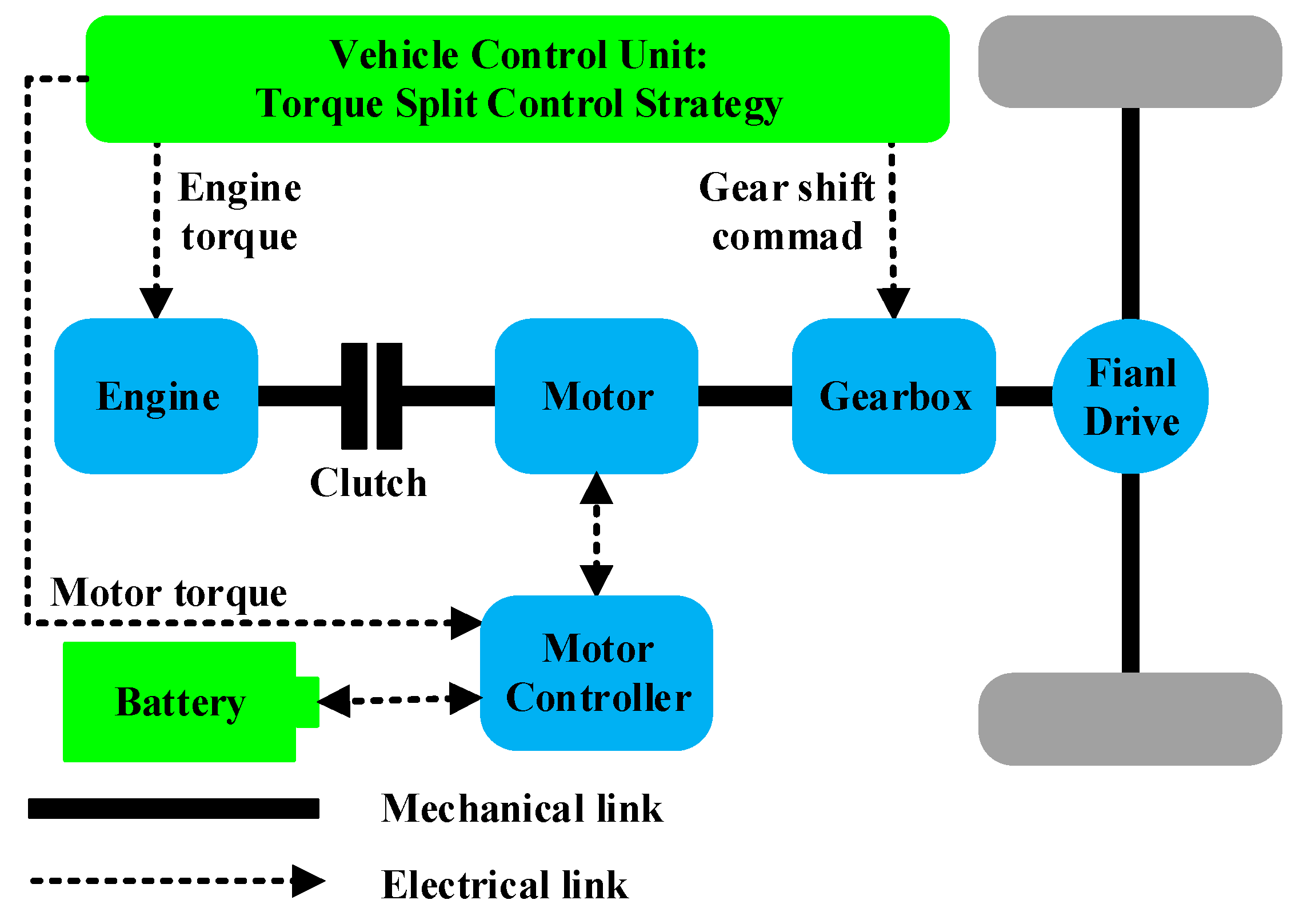
This research selects a torque-coupling parallel HEV as the objective HEV. Vehicle parameters for simulation are listed in Table 1. Figure 1 shows the parallel hybrid powertrain that has a spark ignition engine, an electric motor, a nickel metal hydride battery pack, an automatic clutch, a gearbox, and a final drive. The electric motor is located between the engine and the transmission. In this configuration, the motor rotor works as the torque coupler. When the clutch is engaged, the engine and motor have the same speed. The advantage of this architecture is the elimination of the mechanical torque coupler, which results in a simple and compact drivetrain. This configuration also benefits from abundant operational modes, where the motor functions as an engine starter, along with an electrical generator for regenerative braking and an engine power assistant. Here, a vehicle control unit directly commands the torque required from both power sources of the vehicle. The powertrain information has been shown in [6].
2.2. Optimal Control Problem
In this section, we demonstrate key concepts for the EMS control problem. For example, state vector, control vector, control constraints, and instant cost function.
In this research, we model the parallel HEV as a discrete-time dynamic system as follows:
where represents the current discrete time step; is the total sampling time of the whole driving cycle; is the state variables which summarize past information that is relevant for future optimization; is the control variables, which is the decision to be selected at time step from a given set; is a function according to which the HEV updates. We choose torque demand at the driven wheels from the driver , wheel speed , and battery state of charge as state variables (e.g., ) and engine torque and gear ratio as control variables (e.g., ).
The optimal control problem for this EMS is to find an optimal control sequence to minimize the fuel economy, and constrain the battery SOC within a reasonable scope during a driving cycle. The optimal control action can be obtained by solving the following Bellman equation:
where is the optimal cumulated cost function from time step to the end of the driving cycle. As for the infinite horizon, Equation (2) will change to the following equation:
where is a discount factor, which ensures the total cost function convergence and indicates the importance of future cost to current cost; denotes the cost incurred at time step .
where , and are the fuel consumption and SOC derivation from a desired value from time step to time step , respectively; the weight provides tunable parameters that meet the SOC constraints.
When solving the above optimal control problem, the following boundary conditions should be satisfied to guarantee that the parallel HEV components will work properly:
2.3. Wavelet Transformation Theory
In this section, we will give a brief introduction to a wavelet transformation theory, which is the basis of a CWNN.
If a function satisfies the following item:
where is the Fourier transformation of , which is called a wavelet or mother wavelet.
Given a wavelet , a family of wavelets can be derived with different and from the following equation:
where is a dilation factor and is a translation factor. is called the wavelet basis function.
For a function , we can get its wavelet transform from the following equation:
where is the conjugate function of . is the inner product of and a family of wavelets .
For a common input defined in discrete state, and the dilation set at 2, we can get the following wavelets:
where and .
2.4. Common Wavelet Neural Network
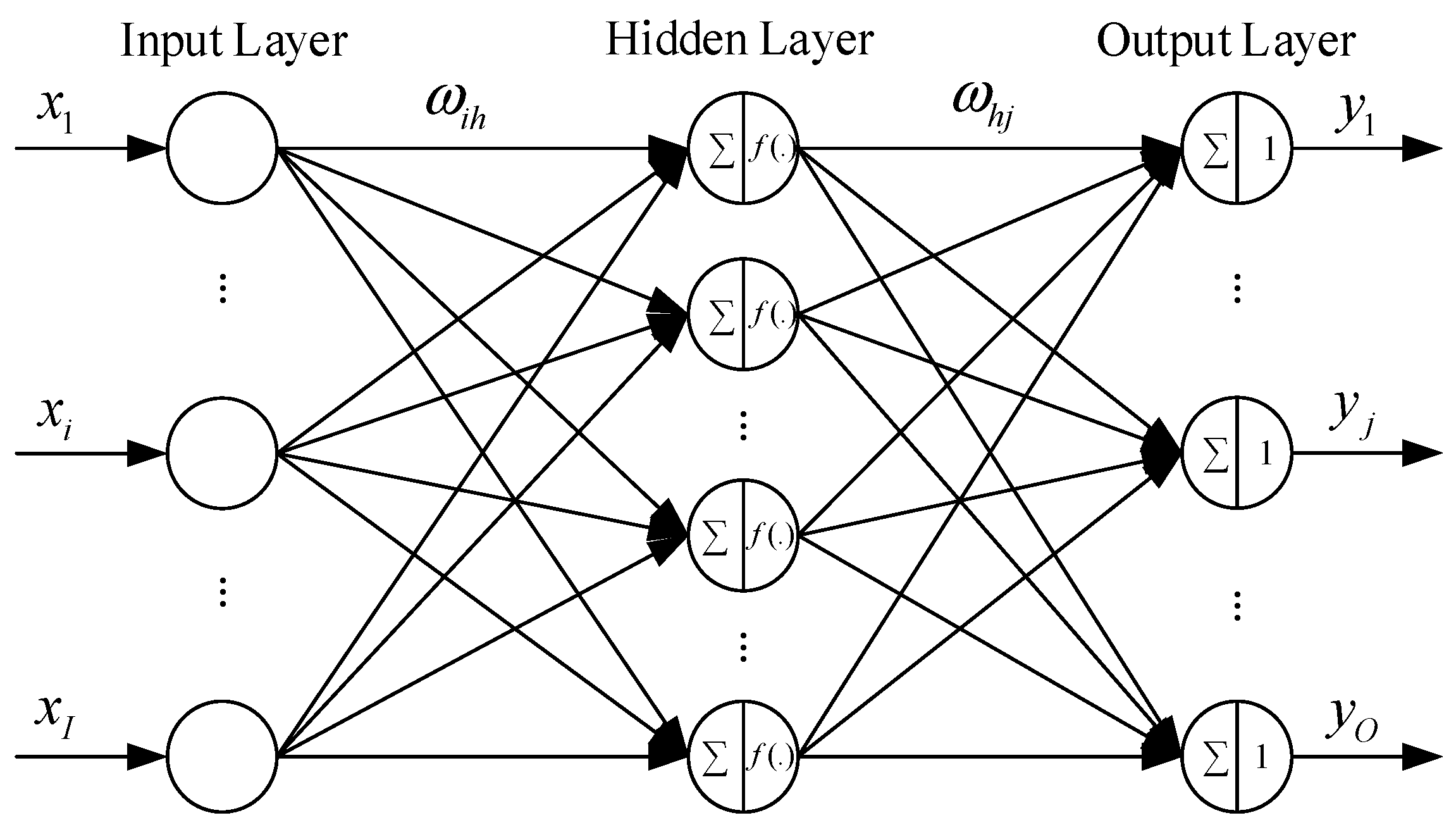
The wavelet neural network is based on a wavelet transformation theory and neural network. Different from broadly used back propagation neural network (BPNN) and RBFNN, a wavelet neural network, which we call a common wavelet neural network (CWNN), utilizes a wavelet function as the activation function in the hidden layer. Compared with a RBFNN, a CWNN does not need a clustering preprocessing on the input data, and has same approximation ability. A commonly used topology of a CWNN is shown in Figure 2.
In the CWNN, the input of hidden layer is as follows:
where is the input vector; and are the total neuron number of the input layer, and hidden layer, respectively; and is the weight factor between the th input neuron and the th hidden layer.
The output of the hidden layer is as follows:
where is the shift factor of the wavelet basis function; is the scaling factor; is the weight factor between input layer to hidden layer; and is the activation function in the hidden layer, which is a wavelet function, such as a Morlet function.
The input of the output layer is as follows:
where is the weight factor between the th hidden neuron and the th output neuron; is the total neuron number of the output layer; is the output vector of the network.
In a CWNN, the weight factors are trained according to a gradient descent algorithm, while the prediction error propagates backwards. The network parameters th training is as follows:
where is the prediction error indication of the network; is the learning rate of the network. Meanwhile, , , and are as follows:
2.5. Multi-Resolution Analysis of Functions
The multi-resolution analysis of functions is based on the theory of multi-resolution analysis proposed by Mallat in [15,16].
Let () is a closed subspace of a square-integrable space at the resolution , which is also the sampling interval. The subspace family has the following features:
- (1)
- Causality and consistency.
- (2)
- Scaling regularity. When we approximate a function with at the resolution , where is a projection of in subspace . Then the following equation will be satisfied:
- (3)
- Gradual completeness.
- (4)
- Orthogonal basis existence.where is a unique function, called a scaling function. Meanwhile, , and .
When we approximate a function with at the resolution , we can conclude the following equation based on Feature (4):
We define be the orthogonal space of in . In other words, and . Then,
where is a projection of on the space . We can say is a detail of function at resolution . Mallat has pointed out that a unique wavelet exists, whose dilations and translations constitute a family of functions . These are the orthonormal basis of space . As a result, we get the following equation:
where is the projection of on the orthonormal basis . We obtain the following equation:
In other words, at the resolution ,
where is the lowest resolution and is the total number of scaling functions. In a real application, we can obtain according to the following equation:
where , and are the maximum and minimum value of . Using Equation (19), we will get the following equation at resolution :
Equations (19) and (21) are the multi-resolution analysis of functions proposed by Moody in [17].
2.6. Multi-Resolution Wavelet Neural Network
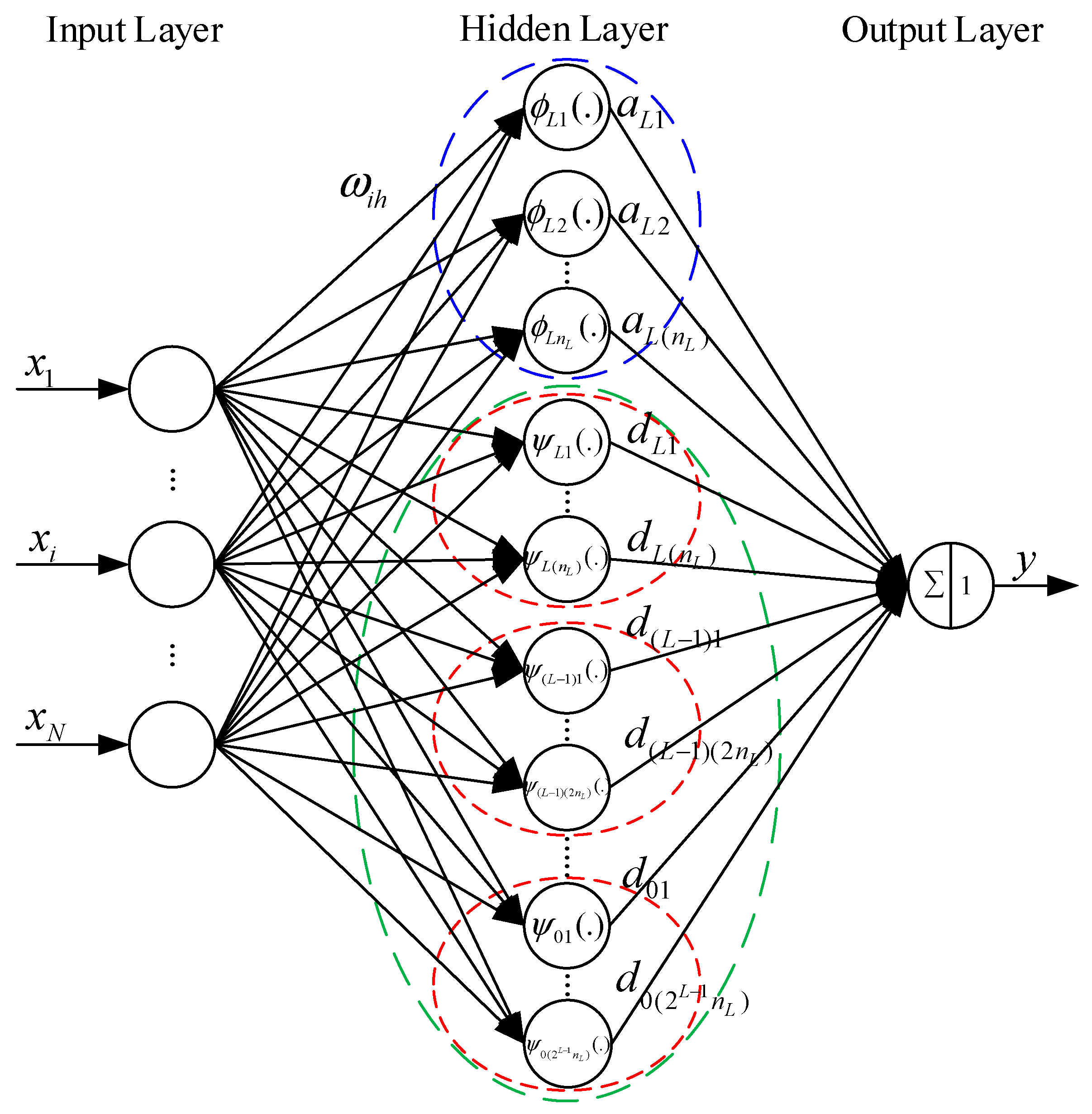
In this research, we proposed a multi-resolution wavelet neural network (MRWNN) based on the theories mentioned in Section 2.4 and Section 2.5. The structure of the proposed MRWNN is shown in Figure 3. Different to RBFNN, the hidden layer in MRWNN contains two types of nodes: wavelet nodes (-nodes, which are in the green ellipse) and scaling nodes (-nodes, which are in the blue ellipse, where one red circle represents the scaling nodes at a same resolution). Compared with RBFNN, the MRWNN does not need a clustering preprocessing for the input data, and enjoys faster convergence and higher approximate accuracy for the orthogonal characteristic of activation function in hidden nodes.
The output of the proposed MRWNN is as follows:
where is the input of the th hidden layer or scaling node; () is the input of the th hidden layer or the th wavelet node.
In real applications, we usually train the network at resolution . If the output does not meet our precision requirements, we keep the scaling nodes and add the detail of resolution at resolution . We proceed like this until the training precision meets our requirements.
In this MRWNN, the weight factors are trained according to the same gradient descent algorithm as in Equations (13) and (14). The weight factor between the th hidden node and the output node is as follows:
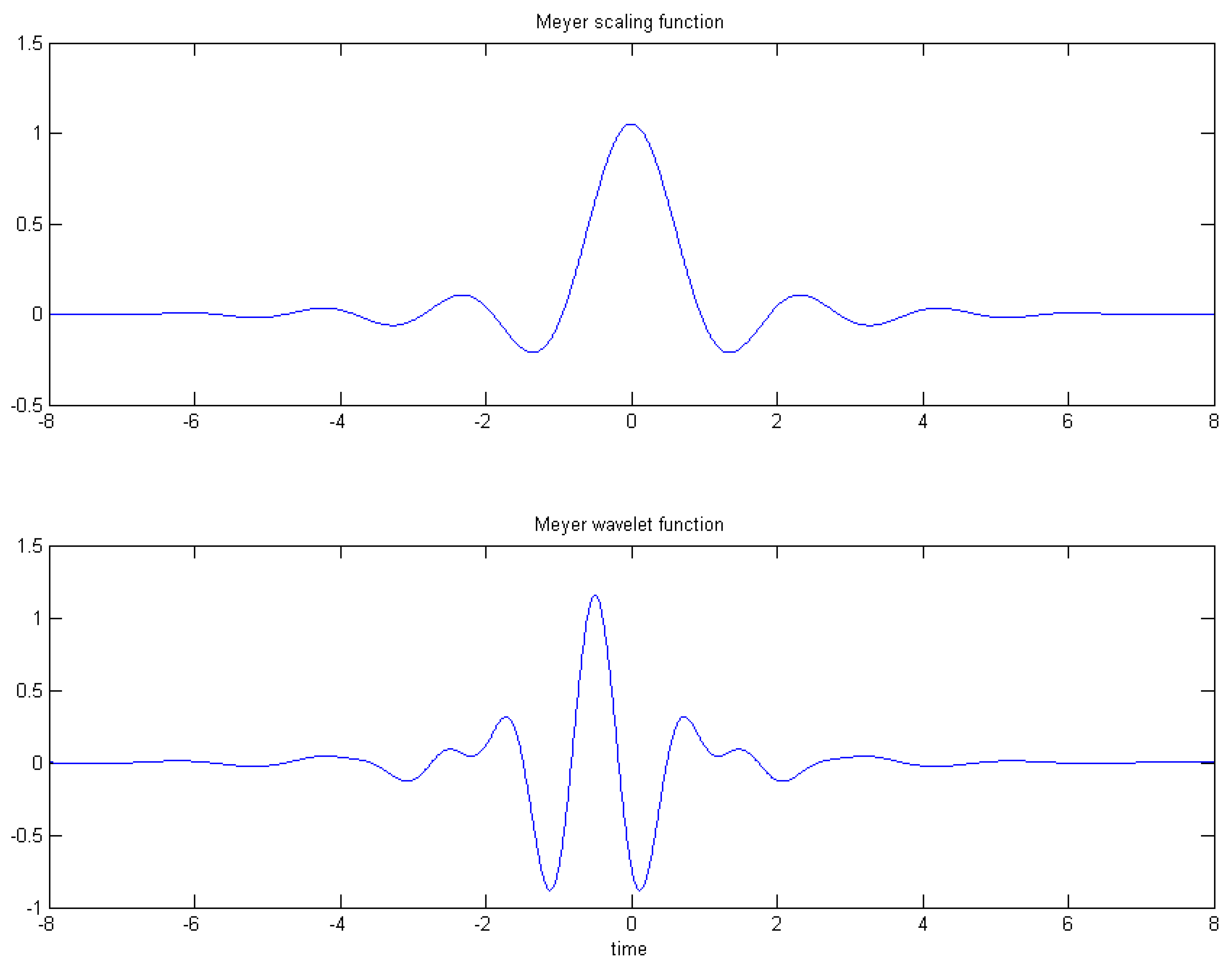
In this research, we use the Meyer wavelet, which is infinitely differentiable with effective support and defined in the frequency domain. In [18], Valenzuela and de Oliveira give the closed analytical expression for the Meyer scaling function and Meyer wavelet function shown as follows:
where is the scaling function. The wavelet function is as follows:
where
The Meyer wavelet and scaling functions in time domain are shown in Figure 4.
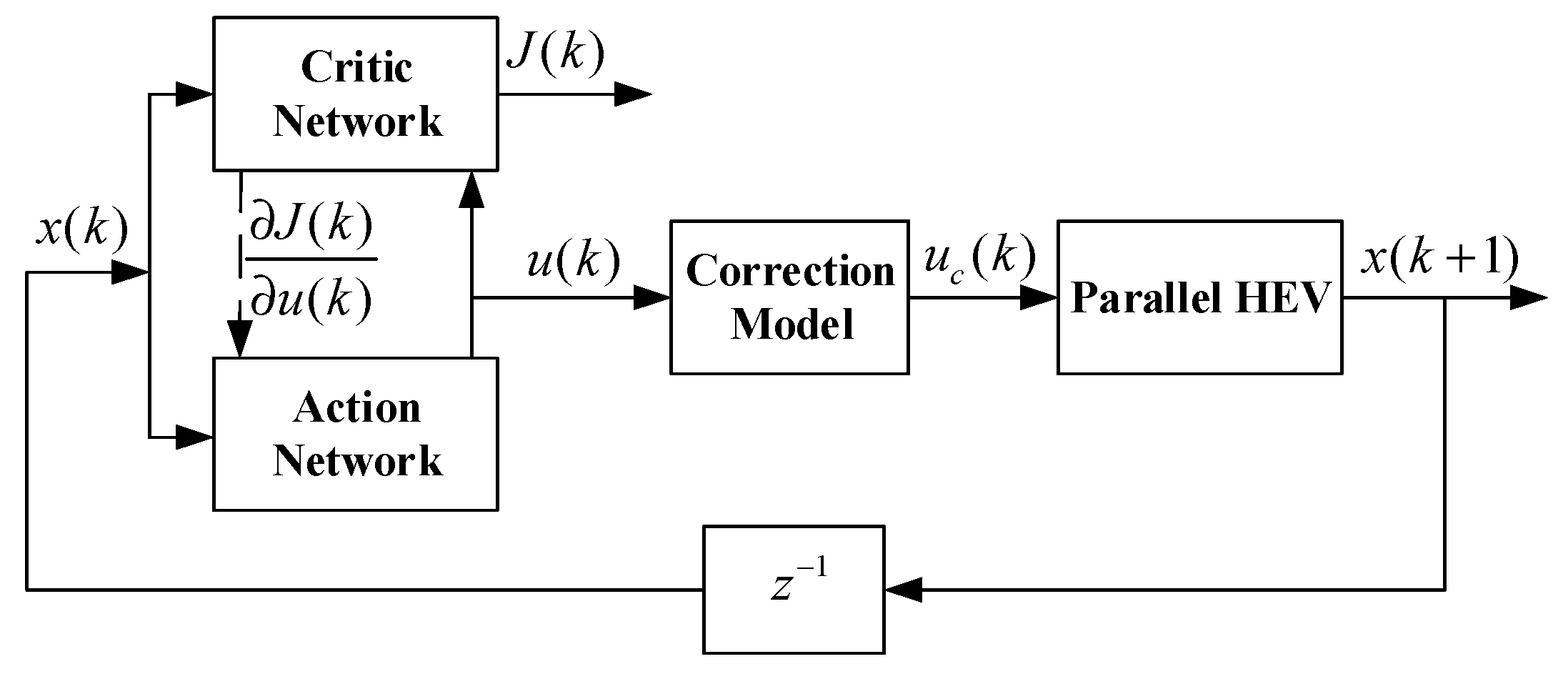
3. Proposed NDP for Parallel HEVs
Figure 5 is the structure of the proposed NDP method, which contains a critic network, an action network, a correction model for the output of action network, and a time delay from time step to time step . The critic network utilizes a MRWNN presented in Section 2.5. The action network utilizes a CWNN, in which the activation function is a Morlet function. The correction model modifies the output variable of action network to fit for Limitation (5). Because the output gear ratio of action network is a continuous variable, we also use the correction model to discretize the continuous gear ratio to the real vehicle gear ratio of the vehicle. The critic network, action network, and implementation procedure of the proposed NDP EMS will be described in this section.
3.1. Critic Network Description
In the NDP method, the critic network is used to get the approximate value of the optimal value function , which is shown in Equation (2), and used in dynamic programming. As a result, we get the following equation:
will be obtained by training the weights of the network according to current state variables and control variables .
In this paper, the critic network is a MRWNN, described in Section 2.5. In this critic network, is the input vector, and is the output vector. The prediction error is defined according to a learning approach as follows:
where is a discount factor; used as a reinforcement signal, is the instantaneous cost, and can be calculated according to Equation (4).
Meanwhile, the prediction error indication of the critic network is defined as follows:
In the critic network, the weight factors (e.g., and ) are adapted according to Equations (13) and (14).
3.2. Action Network Description
The objective of the action network is to find an action to approximate the optimal control shown in Equation (2), which is done by adapting the weights and parameters of the network according to the variation of the output of critic network . In this network, the state vector of the vehicle is the input vector (), and the control vector of the vehicle is the output vector ().
In this paper, the action network is a common wavelet neural network (CWNN) consisting of three layers of neurons—input, hidden, and output layer—as shown in Section 2.4. The adaptation of the action network is achieved by back-propagating the following prediction error :
Meanwhile, the prediction error indication of the action network is defined as follows:
In the action network, the weight factors (e.g., and ) and wavelet function parameters (e.g., and ) are adapted according to the same gradient descent algorithm in Equations (13) and (14).
3.3. NDP Implementation Procedure
The NDP implementation procedure is presented as follows:
- Select an appropriate structure for the critic network and action network separately, which means determining the number of hidden layers. In this design, the number of hidden layers of the critic network and action network is 30 and 11, respectively.
- Initialize the weights and parameters of both networks according to a rule-based EMS. Initialize the output of the critic network, the maximum training error of critic network , the maximum of the norm for weights of action network variation , and maximum times for training both networks, and . In this research, the maximum training times for the action network and critic network are all 50.
- Set the whole iteration time and .
- Set . Calculate the current control vector .
- Set the iteration time of critic network to .
- Set . Calculate the error of critic network and according to Equations (32) and (33). Update the weights and parameters of the critic network according to Equations (13) and (14);
- When or , save the weights and parameters of the critic network as the weights and parameters at time step , and proceed to step 8. Otherwise, return to step 6.
- Set the iteration time of action network to .
- Set . Calculate the error of action network and according to Equations (34) and (35). Update the weights and parameters of the action network according to Equations (13) and (14);
- When or , save the weights and parameters of the critic network as the weights and parameters at time step , and proceed to step 11. Otherwise, return to step 9.
- When the norm of weights for action network variation is less than , save the weights of both networks as the weights at the current time step; otherwise, return to step 4.
4. Results and Discussion
In the simulation test of the proposed NDP-based EMS, the detailed model of the parallel HEV is built in ADVISOR2002 (Advanced Vehicles Simulator) to accurately reflect the vehicle performance, which is based on Simulink. The simulation was carried out on a computer with Intel Core 2 Duo 3.10 GHZ CPU and 32G memory. We have compared the proposed NDP method with the NDP method in [14] to test the proposed NDP based on CWNN and MRWNN. We have also compared the NDP EMS with a SDP method proposed in [6], which is an optimal method, in driving cycles of CYC_UDDS, CYC_1015 and a composite driving cycle, which is composed of a CYC_1015, a CYC_UDDS, and a CYC_WVUCITY driving cycle, to test the optimality of the proposed NDP method.
According to Section 2.2, the orientation of the EMS is to maximize the fuel economy and to satisfy SOC constraint. In simulations, we evaluate fuel economy with miles per gallon (mpg) gasoline equivalent. The SOC constraint is to ensure battery SOC . Meanwhile, we evaluate the component efficiency of the parallel HEV with engine average efficiency, average motoring efficiency, and average generating efficiency.
Table 2 shows the fuel economy and HEV component efficiency of the proposed NDP and NDP EMS in [14] in driving cycles of CYC_UDDS. From Table 2, we can see that the proposed NDP improves fuel economy by about 5.4%, average generating efficiency by about 7.6%, and average motoring efficiency by about 1.2% compared with the NDP in [14]. The two NDP methods keep SOC in nearly the same range of 0.55–0.7. These indicate that the proposed NDP with CWNN and MRWNN has better control results in the UDDS driving cycle than the NDP with RBFNN in [14]. In the NDP in [14], they are 25 and 20. This may be due to the CWNN and MRWNN enjoying better approximation and learning ability in handling nonlinear problems than a RBFNN. To further improve the performance of the proposed NDP EMS, we can increase the maximum training time of the action and critic network, or decrease the training error of the two networks.
Table 3, Table 4 and Table 5 show the fuel economy and component efficiency of SDP, and the proposed NDP-based EMS in driving cycles of CYC_UDDS, CYC_1015, and the composite driving cycle. We can conclude that, compared with the SDP in [6], the proposed NDP EMS improves fuel economy by about 25.9%, 6.2%, and 25.6%, respectively, under CYC_UDDS, CYC_1025, and the composite driving cycle. In the three driving cycles, the proposed NDP and SDP all keep SOC in nearly the same range. The proposed NDP EMS also improves the average generating efficiency by about 6.7%, 5.2%, and 4%, respectively, under CYC_UDDS, CYC_1025, and the composite driving cycle. This shows that the proposed NDP is better than the SDP method. There are three reasons for the simulation results. The first is that the state space and action space are all discretized in SDP and successive in NDP, which reduces the error induced by low discretization resolution. The second reason is that the NDP-based method has generalization ability and improves the generating efficiency in braking. Last but not least, the probability transfer matrix of SDP method is built with the UDDS driving cycle, which induces that the SDP is only suitable for driving cycles with the same probability transfer matrix.
Figure 6 shows the torque demand at the input of gear box, engine torque, motor torque, SOC, and gear ratio variation of proposed NDP EMS results in CYC_UDDS driving cycle. We can see that the engine is in a higher torque output mode most of the time, and the motor provides energy in peak and engine starting times. Battery SOC is constrained in the region of 0.55–0.7, which ensures safe battery usage.
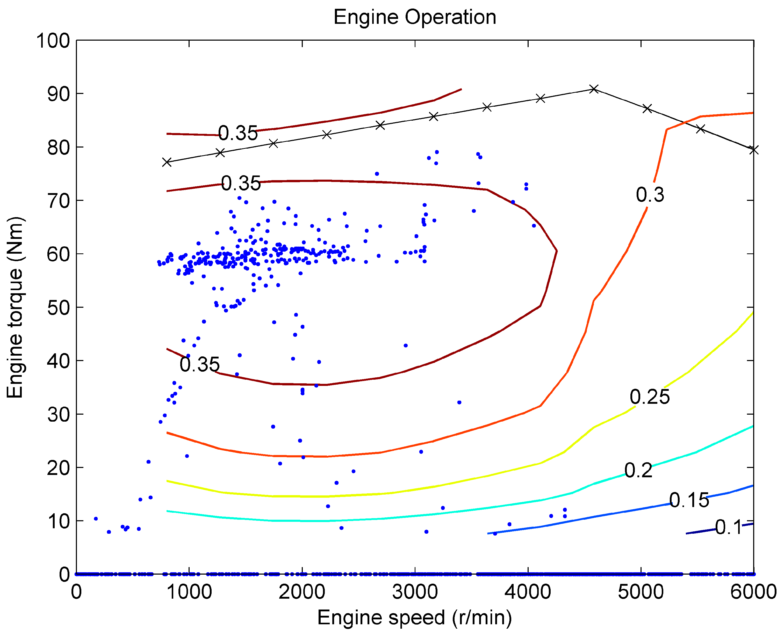
Figure 7 shows the engine operation efficiency in NDP EMS. We can see that, in most situations, the engine is in an efficiency region larger than 0.35.
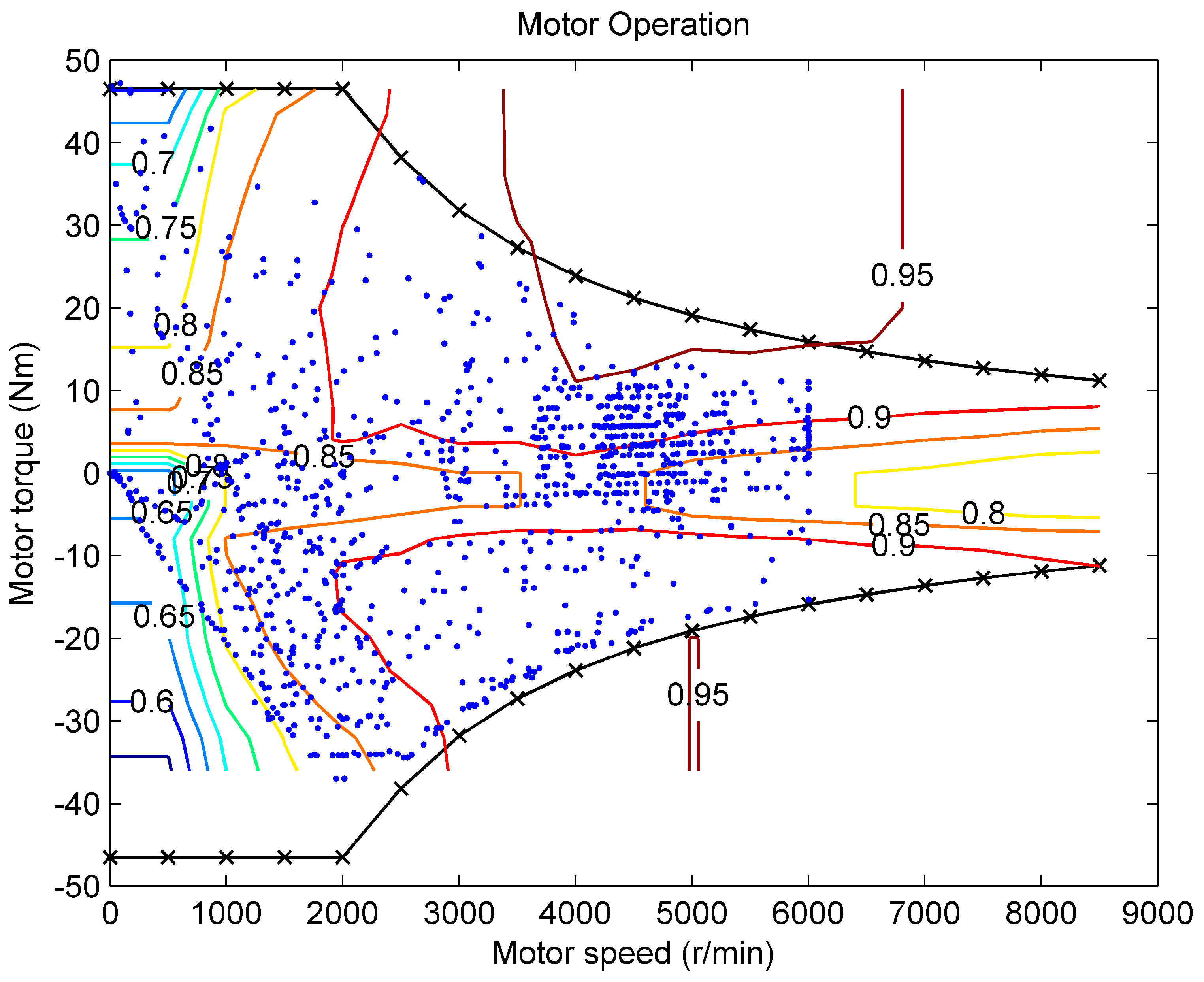
Figure 8 shows the motor operation efficiency in NDP EMS. We can see that, in most situations, the motor is in an efficiency region larger than 0.8. The operation points in the lower efficiency region are distributed uniformly, which coincides with the actual operational points of the motor in real applications.
5. Conclusions
For an HEV, EMS design is critically related to the fuel economy and battery SOC degradation. In this paper, a neuron-dynamic program (NDP) has been designed for the EMS problem of a parallel HEV. In this NDP, a multi-resolution wavelet neural network is used as the critic network to approximate the cumulated value function; a common wavelet neural network is employed to train the optimal action according to current state vector and the output of the action network. A gradient descent algorithm is utilized to train both the neural networks.
ADVISOR2002 simulation results show that the proposed NDP EMS achieves better performance in fuel economy, generating better efficiency and average engine efficiency than the NDP reported before with RBFNN as a critic network and an action network under CYC_UDDS driving cycle. The simulation results also indicate that, compared with the SDP approach in three different driving cycles, the proposed NDP EMS significantly improves fuel economy and average generating efficiency. The NDP method also guarantees battery SOC at a safe range of 0.55–0.7 from the start of one cycle to the end. The performance of the NDP EMS demonstrates the usefulness of the NDP in online applications. The comparison with RBFNN-based NDP EMS confirms the efficiency of the CWNN and MRWNN.
Acknowledgments
This work is supported by the National Key Research and Development Program of China (Grant No. 2016YFD0700602), the Technical Research Foundation of Shenzhen (Grant No. JSGG20141020103523742), the National Natural Science Foundation of China (61573337), and the National Natural Science Foundation of China (61603377).
Author Contributions
Feiyan Qin and Weimin Li conceived the NDP control strategy. Feiyan Qin designed and wrote the whole manuscript. Weimin Li checked the whole manuscript. Guoqing Xu and Yue Hu checked the manuscript.
Conflicts of Interest
The authors declare no conflict of interest.
References
- Chen, J.; Xu, C.; Wu, C.; Xu, W. Adaptive fuzzy logic control of fuel-cell-battery hybrid systems for electric vehicles. IEEE Trans. Ind. Inform. 2018, 14, 292–300. [Google Scholar] [CrossRef]
- Delprat, S.; Lauber, J.; Guerra, T.M.; Rimaux, J. Control of a parallel hybrid powertrain: Optimal control. IEEE Trans. Veh. Technol. 2004, 53, 872–881. [Google Scholar] [CrossRef]
- Kim, N.; Cha, S.; Peng, H. Optimal control of hybrid electric vehicles based on Pontryagin’s minimum principle. IEEE Trans. Control Syst. Technol. 2011, 19, 1279–1286. [Google Scholar]
- Perez, L.V.; Bossio, G.R.; Moitre, D.; Garcia, G.O. Optimization of power management in an hybrid electric vehicle using dynamic programming. Math. Comput. Simul. 2006, 73, 244–254. [Google Scholar] [CrossRef]
- Stephan, U.; Nikolce, M.; Conny, T.; Bernard, B. Optimal energy management and velocity control of hybrid electric vehicles. IEEE Trans. Veh. Technol. 2018, 67, 327–337. [Google Scholar]
- Qin, F.; Xu, G.; Hu, Y.; Xu, K.; Li, W. Stochastic optimal control of parallel hybrid electric vehicles. Energies 2017, 10, 214. [Google Scholar] [CrossRef]
- Munoz, P.M.; Correa, G.; Gaudiano, M.E.; Fernandez, D. Energy management control design for fuel cell hybrid electric vehicles using neural networks. Int. J. Hydrog. Energy 2017, 42, 28932–28944. [Google Scholar] [CrossRef]
- Zhang, Q.; Deng, W.; Li, G. Stochastic control of predictive power management for battery/supercapacitor hybrid energy storage systems of electric vehicles. IEEE Trans. Ind. Inform. 2018. [Google Scholar] [CrossRef]
- Zhang, F.; Xi, J.; Langari, R. Real-time energy management strategy based on velocity forecasts using V2V and V2I communications. IEEE Trans. Control Syst. 2017, 18, 416–430. [Google Scholar] [CrossRef]
- Song, C.; Lee, H.; Kang, C.; Lee, W.; Kim, Y.B.; Cha, S.W. Traffic speed prediction under weekday using convolutional neural networks concepts. In Proceedings of the IEEE Intelligent Vehicles Symposium, Redondo Beach, CA, USA, 11–14 June 2017; IEEE: New York, NY, USA, 2017; pp. 1293–1298. [Google Scholar]
- Tian, H.; Lu, Z.; Huang, Y.; Tian, G. Adaptive fuzzy logic energy management strategy based on reasonable SOC reference curve for online control of Plug-in Hybrid electric city bus. IEEE Trans. Intell. Transp. Syst. 2018. [Google Scholar] [CrossRef]
- Qi, X.; Luo, Y.; Wu, G.; Boriboonsomsin, K.; Brath, M.J. Deep reinforcement learning-based vehicle energy efficiency autonomous learning system. In Proceedings of the 2017 IEEE Intelligent Vehicles Symposium (IV), Redondo Beach, CA, USA, 11–14 June 2017. [Google Scholar]
- Hu, Y.; Li, W.; Xu, K.; Zahid, T.; Qin, F.; Li, C. Energy management strategy for a hybrid electric vehicle based on deep reinforcement learning. Appl. Sci. 2018, 8, 187. [Google Scholar] [CrossRef]
- Li, W.; Xu, G.; Xu, Y. Online learning control for hybrid electric vehicle. Chin. J. Mech. Eng. 2012, 25, 98–106. [Google Scholar] [CrossRef]
- Mallat, S.G. Multiresolution approximations and wavelet orthogonal bases of L2(R). Trans. Am. Math. Soc. 1989, 315, 67–87. [Google Scholar]
- Mallat, S.G. A theory for multiresolution signal decomposition: The wavelet representation. IEEE Trans. Pattern Anal. Mach. Intell. 1989, 11, 674–693. [Google Scholar] [CrossRef]
- Moody, J. Fast Learning in Multi-Resolution Hierarchies; research report; Yale University: New Haven, CT, USA, 1989. [Google Scholar]
- Valenzuela, V.V.; Oliveira, H.M. Close expressions for Meyer wavelet and scale function. arXiv, 2015; arXiv:1502.00161. [Google Scholar]
Figure 1.
Configuration of the parallel HEV powertrain.

Figure 2.
Topology of CWNN.

Figure 3.
Structure of multi-resolution wavelet neural network (MRWNN).

Figure 4.
Meyer wavelet function and scaling function in the time domain.

Figure 5.
Structure of the proposed NDP method.

Figure 6.
NDP EMS simulation results under CYC_UDDS driving cycle.
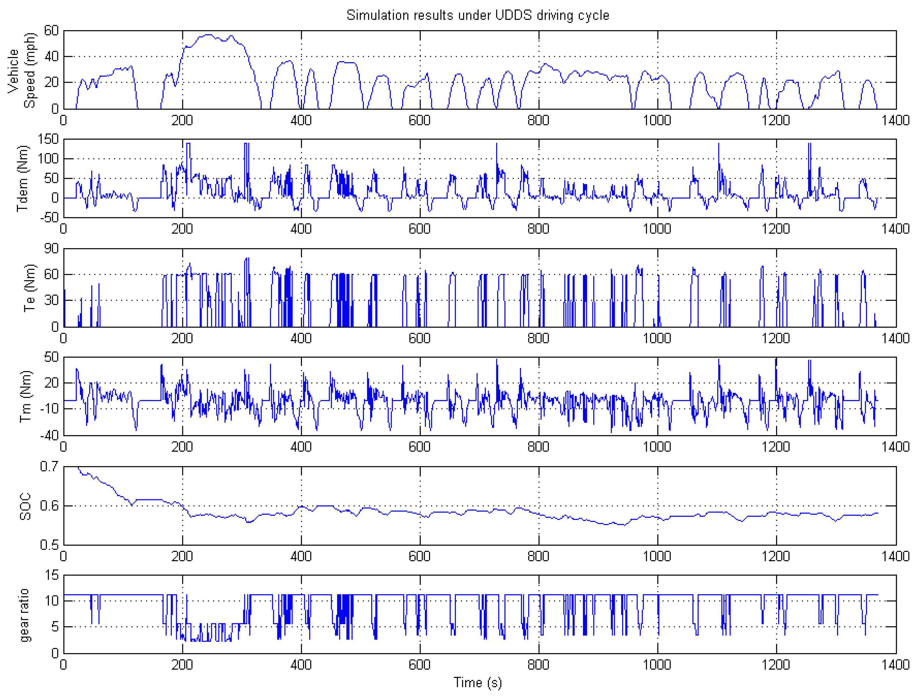
Figure 7.
Engine efficiency in NDP EMS under the CYC_UDDS driving cycle.

Figure 8.
Motor efficiency in NDP EMS under the CYC_UDDS driving cycle.


Table 1.
Parameters of the parallel HEV.
| Item | Value |
|---|---|
| Final drive gear efficiency (%) | 0.9296 |
| wheel radius (m) | 0.275 |
| Coefficient of aerodynamic drag | 0.25 |
| Vehicle frontal area (m2) | 1.9 |
| Air density (kg/m3) | 1.2 |
| Rolling resistance coefficient | 0.0054 |
| Vehicle mass (kg) | 1000 |
Table 2.
Control orientation improvement with other NDP EMS.
| EMS | NDP in [14] | Proposed NDP |
|---|---|---|
| Fuel Economy (mpg) | 81.6 | 86.0 |
| SOC range | 0.55–0.7 | 0.54–0.7 |
| Engine Eff. (%) | 34.6 | 35.0 |
| Motoring Eff. (%) | 91.6 | 86.1 |
| Generating Eff. (%) | 92.7 | 99.7 |
Table 3.
Control orientation improvement with another optimal method under CYC_UDDS.
| EMS | SDP | Proposed NDP |
|---|---|---|
| Fuel Economy (mpg) | 68.3 | 86.0 |
| SOC range | 0.54–0.7 | 0.54–0.7 |
| Engine Eff. (%) | 35.7 | 35.0 |
| Motoring Eff. (%) | 91.1 | 86.1 |
| Generating Eff. (%) | 93.4 | 99.7 |
Table 4.
Control orientation improvement with another optimal method under CYC_1015.
| EMS | SDP | Proposed NDP |
|---|---|---|
| Fuel Economy (mpg) | 58.2 | 61.8 |
| SOC range | 0.54–0.7 | 0.55–0.7 |
| Engine Eff. (%) | 36.1 | 33.5 |
| Motoring Eff. (%) | 87.0 | 88.6 |
| Generating Eff. (%) | 90.5 | 95.2 |
Table 5.
Control orientation improvement with another optimal method under CYC_1015 + CYC_UDDS + CYC_WVUCITY.
Table 5.
Control orientation improvement with another optimal method under CYC_1015 + CYC_UDDS + CYC_WVUCITY.
| EMS | SDP | Proposed NDP |
|---|---|---|
| Fuel Economy (mpg) | 62.1 | 78.0 |
| SOC range | 0.54–0.7 | 0.53–0.7 |
| Engine Eff. (%) | 36.3 | 36.1 |
| Motoring Eff. (%) | 86.1 | 83.7 |
| Generating Eff. (%) | 91.8 | 95.5 |
© 2018 by the authors. Licensee MDPI, Basel, Switzerland. This article is an open access article distributed under the terms and conditions of the Creative Commons Attribution (CC BY) license (http://creativecommons.org/licenses/by/4.0/).
Share and Cite
MDPI and ACS Style
Qin, F.; Li, W.; Hu, Y.; Xu, G. An Online Energy Management Control for Hybrid Electric Vehicles Based on Neuro-Dynamic Programming. Algorithms 2018, 11, 33. https://doi.org/10.3390/a11030033
AMA Style
Qin F, Li W, Hu Y, Xu G. An Online Energy Management Control for Hybrid Electric Vehicles Based on Neuro-Dynamic Programming. Algorithms. 2018; 11(3):33. https://doi.org/10.3390/a11030033
Chicago/Turabian StyleQin, Feiyan, Weimin Li, Yue Hu, and Guoqing Xu. 2018. "An Online Energy Management Control for Hybrid Electric Vehicles Based on Neuro-Dynamic Programming" Algorithms 11, no. 3: 33. https://doi.org/10.3390/a11030033
Note that from the first issue of 2016, this journal uses article numbers instead of page numbers. See further details here.