Combinatorial GVNS (General Variable Neighborhood Search) Optimization for Dynamic Garbage Collection

Abstract

General variable neighborhood search (GVNS) is a well known and widely used metaheuristic for efficiently solving many NP-hard combinatorial optimization problems. We propose a novel extension of the conventional GVNS. Our approach incorporates ideas and techniques from the field of quantum computation during the shaking phase. The travelling salesman problem (TSP) is a well known NP-hard problem which has broadly been used for modelling many real life routing cases. As a consequence, TSP can be used as a basis for modelling and finding routes via the Global Positioning System (GPS). In this paper, we examine the potential use of this method for the GPS system of garbage trucks. Specifically, we provide a thorough presentation of our method accompanied with extensive computational results. The experimental data accumulated on a plethora of TSP instances, which are shown in a series of figures and tables, allow us to conclude that the novel GVNS algorithm can provide an efficient solution for this type of geographical problem.

1. Introduction

Many complex real world problems can be formulated as combinatorial optimization (CO) problems. Technically, CO problems require a proper solution from a discrete finite set of feasible solutions in order to simultaneously achieve the minimization (or maximization) of a cost function and the satisfaction of the problem’s given constraints. One such problem is finding the shortest path (or a path “close” to the shortest with respect to some appropriate metric) for a global positioning system (GPS) in a short period of time. The above real-world problem can be perfectly modeled by the travelling salesman problem (TSP).

The travelling salesman problem (TSP) is one of the most widely studied combinatorial optimization problems. Solving the TSP means finding the minimum cost route so that the salesman (the person or entity who travels along a specific route containing many nodes) can start from a point of origin and return to the origin after passing from all given nodes once. The first use of the term “travelling salesman problem” appeared around 1931–1932. Remarkably, a century earlier, in 1832, a book was printed in Germany [1], which, although dedicated to other issues, in the last chapter deals with the essence of the TSP problem: “With a suitable choice and route planning, you can often save so much time [making] suggestions [...]. The most important aspect is to cover as many locations [as possible], without visiting a location [a] second time.” In that book, the TSP is expressed for the first time using some examples of routes through Germany and Switzerland. However, an in-depth study of the problem is not attempted in this book. The TSP was expressed mathematically for the first time in the 19th century by Hamilton and Kirkman [1]. A cycle in a graph is a closed path that starts and ends at the same node and visits every other node exactly once. A cycle containing all vertices of the graph is called Hamiltonian.

In short, TSP is the problem of finding the shortest Hamiltonian cycle. The Hamiltonian graph problem, i.e., deciding whether a graph has a Hamiltonian cycle, is reducible to the TSP. One can see this by assigning zero length to the edges of the graph and constructing a new edge of length, one for each missing edge. If the solution of the TSP for the resulting graph is zero, then the original graph contains a Hamiltonian cycle; if it is a positive number, then the original graph contains no Hamiltonian cycle [2]. TSP is NP-hard and is of great significance in various fields, such as operational research and theoretical computer science. In practice, TSP amounts to finding the best way one can visit all the cities, return to the starting point, and minimize the cost of the tour.

Typically, TSP is represented by a graph. Specifically, the problem is stated in terms of a complete graph $G=(V,A)$, in which $V=\{v_1,v_2,\dots ,v_n\}$ is the set of nodes and $A=\{(v_i,v_j):v_i,v_j\in V$ and $v_i\ne v_j\}$ is the set of the directed edges or arcs. Each arc is associated with a weight $c_{ij}$ representing the cost (or the distance) of moving from node i to node j. If $c_{ij}$ is equal to $c_{ji}$, the TSP is symmetric (sTSP); otherwise, it is called asymmetric (aTSP). The fact that TSP is NP-hard implies that there is no known polynomial-time algorithm for finding an optimal solution regardless of the size of the problem instance [3].

Real world problems, such as those related to GPS, can be formulated as instances of the TSP. This class of routing problems requires good solutions computed in a short amount of time. In order to improve the computational time, it is common practice to sacrifice some of the solution’s quality by adopting heuristic and metaheuristic approaches [4,5,6]. Heuristics are fast approximation computational methods divided into construction and improvement heuristics. Construction heuristics are used to build feasible initial solutions, and improvement heuristics are applied to achieve better solutions. It is customary to apply improvement heuristics iteratively. Metaheuristics are general optimization frameworks that can be appropriately modified in their individual characteristics in order to generate efficient methods for solving specific classes of optimization problems.

The main contribution of this paper is the application of the novel extension of general variable neighborhood search (GVNS for short) metaheuristic to a GPS problem. We achieve efficient solutions in a short period of time for a GPS application used for garbage trucks, which is modeled as an instance of the TSP. The proposed method guarantees optimal or near-optimal solutions for a real life routing application. GPS applications typically use the nearest neighbor (NN) or some of its variations in order to achieve good results for the routing section. The routing section is a critical part of a typical GPS application because, if the provided routes are optimal or near-optimal, then the end result will also be near-optimal. The routing solutions produced by the GVNS were compared to the ones obtained by the well known NN algorithm and some of its most widely used variations. The computational results reveal that both GVNS’s first and best improvement solutions provide efficient routes that are either optimal or near-optimal and outperform with a wide margin classic, widely used methods, such as NN and its modifications. This novel GVNS is a quantum-inspired expansion of the conventional GVNS in which the shaking function is based on complex unit vectors.

This paper is organized as follows. In Section 2 we present related works, in Section 3 we explain metaheuristics and the variable neighborhood search, and we describe our algorithm in detail. A GPS application and the specific problem we tackle with our algorithm is presented in Section 4. In Section 5, the experimental results of our implementation are presented in a series of matrices and figures that clearly demonstrate that our method outperforms standard approaches like the NN algorithm. Finally, conclusions and ideas for future work are described in Section 6.

2. Related Work

The research community has shown great interest in solving tangible, real world problems via methods applicable to CO problems. Recently, many authors have been actively trying to enhance conventional optimization methods by introducing principles and techniques originating from unconventional methods of computation in the hope that they would prove superior to traditional approaches. For example, Sandip et al. [7] proposed several novel techniques which they called quantum-inspired ant colony optimization, quantum-inspired differential evolution, and quantum-inspired particle swarm optimization, respectively, for multi-level color image thresholding. These techniques find optimal threshold values at different levels of thresholding for color images.

A new quantum-inspired social evolution (QSE) algorithm was proposed by hybridizing a well-known social evolution algorithm with an emerging quantum-inspired evolutionary one. The proposed QSE algorithm was applied to the 0–1 knapsack problem and the performance of the algorithm was compared to various evolutionary, swarm, and quantum-inspired evolutionary algorithmic variants. Pavithr and Gursaran claim that the performance of the QSE algorithm is better than or at least comparable to the different evolutionary algorithmic variants it was tested against [8].

Wei Fang et al. proposed a decentralized form of quantum-inspired particle swarm optimization with a cellular structured population for maintaining population diversity and balancing global and local search [9]. Zheng et al. conducted an interesting study by applying a novel hybrid quantum-inspired evolutionary algorithm to a permutation flow-shop scheduling problem. They proposed a simple representation method for the determination of job sequence in the permutation flow-shop scheduling problem based on the probability amplitude of qubits [10].

Lu et al. designed a quantum-inspired space search algorithm in order to solve numerical optimization problems. In their algorithm, the feasible solution is decomposed into regions in terms of quantum representation. The search progresses from one generation to the next, while the quantum bits evolve gradually to increase the probability of region selection [11]. Wu et al. in [12] proposed a novel approach using a quantum-inspired algorithm based on game-theoretic principles. In particular, they reduced the problem they studied to choosing strategies in evolutionary games. Quantum games and their strategies seem very promising, offering enhanced capabilities over classic ones [13].

Solutions based on variable neighborhood search (VNS) have been applied to route planning problems. Sze et al. proposed a hybrid adaptive variable neighborhood search algorithm for solving the capacitated vehicle routing problem (VRP) [14]. A two-level VNS heuristic has been developed in order to tackle the clustered VRP by Defryn and Sorensen [15]. In [16], a VNS approach for the solution of the recently introduced swap-body VRP is proposed. Curtin et al. made an extensive comparative study of well known methods and ready-to-use software and they concluded that no software or classic method can guarantee an optimal solution to the TSP problems that model GIS problem with more than 25 nodes [17]. Papalitsas et al. proposed a GVNS approach for the TSP with time windows [4] and a quantum-inspired GVNS (qGVNS) for solving the TSP with time windows [18].

Moreover, the proposed method can also be applied on other classes of problems from real world, such as optimization on localization in hospitals, smart cities, and smart parking systems. Tsiropoulou et al. applied RFID technologies to tag-to-tag communication paradigms in order to achieve improved energy-efficiency and operational effectiveness [19]. Liebig et al. presented a system for trip planning that consolidates future traffic threats [20]. Specifically, this system measures traffic flow in areas with low sensor coverage by using a Gaussian Process Regression. Many studies also deal with the optimization of localization and positioning of doctors and nurses in hospitals and health care organizations [21,22].

In this work we demonstrate that, for small problems, our method achieves the optimal value; for larger problems, it guarantees a close to optimal solution with a deviation of 1–3%.

3. Novel Variable Neighborhood Search

In this section, we describe the proposed VNS method version. For completeness, we state the necessary background notions and formal definitions (such as on metaheuristics and VNS).

3.1. Metaheuristics

A metaheuristic is a high-level heuristic, designed to find, create, or select a lower level heuristic (for example a local search algorithm), which can provide an adequate solution to an optimization problem. It is particularly useful for instances with missing or incomplete information, or when the computing capacity is limited. According to the literature on metaheuristic optimization [23], the word “metaheuristics” was devised and proposed by Glover. Metaheuristic algorithms are able to make assumptions about the optimization problem to be solved and thus can be used for a wide variety of problems. Obviously, compared with exact methods, metaheuristic procedures do not guarantee a global optimal solution for each category of problems [24].

Many metaheuristic algorithms apply some form of stochastic optimization. This implies that the generated solution depends on a set of random variables. By searching in a large set of feasible solutions, the metaheuristic procedures can often find good solutions with less computational effort than exact algorithms, iterative methods, or simple heuristic procedures. Therefore, metaheuristic procedures are useful approaches for optimization problems in many practical situations.

3.2. Variable Neighborhood Search (VNS)

VNS is a metaheuristic for solving combinatorial and global optimization problems, proposed by Mladenovic and Hansen [25,26]. The main idea of this framework is the systematic neighborhood change in order to achieve an optimal (or a close-to-optimal) solution [27]. VNS and its extensions have proven their efficiency in solving many combinatorial and global optimization problems [28].

Each VNS heuristic consists of three parts. The first one is a shaking procedure (diversification phase) used to escape local optimal solutions. The next one is the neighborhood change move, in which the following neighborhood structure that will be searched is determined; during this part, an approval or rejection criterion is also applied on the last solution found. The third part is the improvement phase (intensification) achieved through the exploration of neighborhood structures through the application of different local search moves. Variable neighborhood descent (VND) is a method in which the neighborhood change procedure is performed deterministically.

GVNS is a VNS variant where the VND method is used as the improvement procedure. GVNS has been successfully tested in many applications, as several recent works have demonstrated [29,30].

3.3. Description of Our Algorithm

As does the original GVNS, our version of GVNS consists of a VND local search, a diversification procedure, and a neighborhood change step. In our method, the pipe-VND (exploitation in the same neighborhood while improvements are also being made) is used during the improvement phase. During the improvement phase of the pipe-VND, two classic local search strategies are applied: the relocate and the 2-opt. In the relocate, the solutions are obtained by removing a node and inserting it in a different position of the current route. In the 2-opt, the solutions are obtained by breaking two edges and reconnecting them in a different order.

The biggest difference between our approach and the classic GVNS is in the diversification phase. The main use of a shaking function is to resolve local minima traps within a VNS procedure. In our approach, perturbation is achieved by adopting techniques from the field of quantum computation.

Quantum-inspired procedures are not actual quantum algorithms designed to run on future quantum computers, but conventional, classical algorithms that utilize principles and ideas from the field of quantum computing. Quantum computing was envisioned by Feynman [31,32], who was the first to observe that it is not possible to efficiently simulate an actual quantum system using a classical computer. More in-depth information regarding quantum computation and its principles can be found in [33,34].

In our case, during each shaking call, a simulated quantum n-qubit register generates a complex n-dimensional unit vector. A quantum register is the quantum analogue of a classical processor register. The dimension n of the complex unit vector is greater than or equal to the dimension of the problem. Our algorithm takes as input the complex n-dimensional vector and produces a real n-dimensional vector. The i-th component, $1\le i\le n$, of the real vector is equal to the modulus squared of the i-th component of the complex vector. Obviously, the components of the real vector are real numbers in the interval $[0,1]$.

Each node of the current solution is associated with precisely one of the components of the real n-dimensional vector. In effect, the vector components are used as a flag for each node in the current solution. Under this correspondence between vector components and nodes, the sorting of the components of the real vector, will induce an identical ordering among the nodes in the solution. Thus, the ordered route produced after this shaking move will drive our exploration effort in another search space.

At this point, it should be mentioned that the NN heuristic is used in order to produce an initial feasible solution (the first node is set as a depot). From an algorithmic perspective, the procedure is summarized in the next pseudocode fragment [35]. The solution method is provided in Algorithm 1:

Algorithm 1: Pseudocode of the novel general variable neighborhood search (GVNS)

4. GPS Application for Garbage Trucks Modeled as a Travelling Salesman Problem

An operation with substantial importance for the handling of everyday scheduling of a city’s traffic is the routing of garbage trucks from their depots to every dustbin on their routes and back to their depots. The optimal routes correspond to minimum required transportation time and minimum distance. Finding optimal routes typically proves to be time-consuming, especially in the case of metropolitan cities with very dense road networks. However, by exploiting recent advances from the field of metaheuristics, it is possible to attain efficient, near-optimal solutions in a short amount of time for many practical cases. We take advantage of the performance improvement brought by a novel metaheuristic procedure based on VNS. Our novel GVNS, in combination with the minimal required computational time, can provide a significantly enhanced the solution for these kind of problems. The incorporation of the enhanced VNS procedure within the GIS will lower the system’s response time and provide close to optimal solutions.

GIS technology integrates common database operations such as query and statistical analysis with the unique visualization and geographic analysis benefits offered by maps [36,37]. Among other things, a GIS facilitates the modeling of spatial networks (e.g., road networks) offering algorithms to query and analyze them. Spatial networks are modeled with graphs. In the case of road networks, the graph’s arcs correspond to street segments, whereas the nodes correspond to street segment intersections. Each arc has a weight associated with it, representing the cost of traversing it.

A GIS usually provides a number of tools for the analysis of spatial networks. It generally offers tools to find the shortest or minimum route through a network and heuristic procedures to find the most efficient route to a series of locations. Such a problem is typically modeled as an instance of the TSP. Our implementation solves efficiently the TSP problem, finding near-optimal solutions for a range of small, medium, or large benchmark problems. Distance matrix calculation can be used to calculate distances between pairs of nodes representing origins and destinations, whereas location-allocation functions determine site locations and assign demand to sites. These capabilities of GIS for analyzing spatial networks enable them to be used as decision support systems for the districting and routing of vehicles [38,39].

Routing a garbage truck from its depot to each dustbin and back is modeled by finding routes for the travelling salesman problem. The GIS will be used to find the optimal routes corresponding to minimum required transportation time. The GIS can also present the driver with directions corresponding to the routes generated. These directions will be transmitted to the garbage truck. In a real-time system, the time performance of the routing function is of vital significance. Metaheuristics, like our implementation presented here, can guarantee that.

Our Approach

In this paper, we describe a system offering a solution to the problem of garbage truck routing management. It is based on quantum-inspired metaheuristics applied on TSP and integrated to GIS/GPS technologies. Our approach is an integrated waste management solution. Based on the functional requirements and some case studies, [40], the components of our application are designed and decomposed into subsystems and smaller functional units. Operations and relationships between subsystems are defined for each subsystem:

• Bin Sensors: equipment that estimates the waste bin fill level and collects, stores, and transmits bins data. This will help our main system to take into account specific bins and avoid computation on final route empty bins.
• Data Gathering from Bins: a unit that communicates with the bin sensors and delivers the collected information to the central system. It can be installed on passing vehicles and consists of three components:
  • a communicator, which implements the communication with the bin;
  • a storage procedure, which temporarily stores the data until transferred to the central system;
  • a transfer procedure, which implements the data transfer to the central system.
  All these operations will be applied via the Global System for Mobile Communications (GSM) network.
• GPS Navigation Applications Integrated in Trucks: a classic navigation application through GPS and will provide navigation guidance to a truck driver and instructions regarding which bins should be collected.
• A Central System: the back-end system of our application. Its main part is the data storing, bin data, vehicle data, and all data needed to compute the most efficient routes. Furthermore, data storing will keep any information retrieved from other subsystems, particularly from the data mining subsystem and the routing optimizations subsystem. All generated spatial information for the current route will be stored locally in a spatial database.
• A Map Substructure: A REST-ful API based on maps that will provide all the required functionality for creating rich-web applications based on geographic and descriptive data.
• A Data Mining Subsystem: a system mainly used to estimate the fullness of bins when we do not have the available information updated.
• A Routing Optimization Structure: Our main contribution is mainly based on implementing efficient routing algorithms for this application. We propose this novel metaheuristic, which provides optimal or close to optimal solutions over a short period of time. Our implementation of routing functionality gives an overall comparative advantage compared with the other implementations for two main reasons:
  • We can compute efficient solutions in a short period of time. This makes the application efficient because we can compute and re-compute, live and continuously, many times for the same route and feed the results to the application.
  • Our routing algorithm outperforms classic methods, such as the NN, that are used to find routes on GPS, and the solutions for every class of problem are near-optimal.

A real-time system like ours must be able to give prompt replies to such queries because, in these situations, the response time is of vital importance. By using efficient local search structures and the novel GVNS for the problem tour, the metaheuristic algorithm can provide better results.

Most GIS/GPS implementations use either the NN or one of its variations to compute routes. NN is a well known and widely used construction heuristic in network designing problems. Initially, in NN, an arbitrary node is inserted in the route as the starting node, and then, iteratively, the nearest to the last added node, selected to insert in the route. The procedure is terminated when all the nodes have been added in the route. Therefore, because of the popularity of NN, when we test the performance of our algorithm, we compare its results both with the optimal solution and the solutions achieved by NN. This comparison demonstrates that GVNS produces results that, in all cases, are near-optimal and significantly superior to the NN algorithm, which is widely used by most GIS/GPS software. As a result of these better routing solutions, the total amount of fuel is drastically reduced. Thus, our method is environmentally friendly, since fuel consumption has a direct impact on the environment.

5. Experimental Results

This section is devoted to the presentation of the experimental results that showcase the strengths of the novel GVNS. The experimental tests were implemented in Fortran 90 and ran on a laptop PC with an Intel Core i7-6700HQ Processor at 2.59 GH and 16 GB memory. We ran each benchmark at least five times and imposed a limit of 60 s per run. We chose this threshold for two reasons. First, it is adequate to compute an optimal or near-optimal solution, and, second, it is short enough to allow for repeated experiments. We then kept the best solution found and computed the average of all runs in order to derive the final cost. The algorithms were tested on 48 benchmark instances from the TSPLIB. TSPLIB is a library that contains a collection of benchmarks for the TSP. These benchmarks are characterized by their diversity and their variation with respect to the dimension of the problem. It is precisely for these qualities that they are widely used by researchers for comparing results [41].

5.1. Novel GVNS versus Nearest Neighbor

In this work, we propose a novel GVNS version based on quantum computing principles and techniques, and we apply it to a garbage collection application, an actual GPS-based problem. Below we present the computational results of our approach. As already mentioned, NN and its variants are widely used in GPS/GIS applications in order to construct the tour of the underlying graph. In particular, we compare our method against the NN heuristic and two of its most well-known variants: the repeated NN and the improved NN. This section presents the comparative analysis among NN, GVNS, and the optimal value (OV), showing the results in a series of figures and tables. It is important to point out that we chose to examine the NN because of its widespread use in GPS applications.

Table 1. The computational results demonstrate that novel GVNS outperforms NN on all TSP instances.

Benchmark Name	NN	Gap NN vs. OV	GVNS BI	Gap GVNS BI vs. OV	GVNS FI	Gap GVNS FI vs. OV	OV
a280	3157	−0.2241	2779	−0.0775	2766	−0.0725	2579
att48	12,861	−0.2101	10,645	−0.0016	10,654	−0.0024	10,628
bayg29	2005	−0.2453	1610	0.0000	1610	0.0000	1610
bays29	2258	−0.1178	2020	0.0000	2020	0.0000	2020
bier127	135,737	−0.1475	121,393	−0.0263	121,551	−0.0276	118,282
kroA100	27,807	−0.3065	21,664	−0.0179	21,774	−0.0231	21,282
burma14	4501	−0.3544	3454	−0.0394	3454	−0.0394	3323
ch130	7579	−0.2404	6342	−0.0380	6373	−0.0430	6110
ch150	8191	−0.2547	6849	−0.0492	6871	−0.0525	6528
d493	41,666	−0.1903	37,715	−0.0775	37,882	−0.0823	35,002
kroB100	29,158	−0.3169	22,514	−0.0168	22,786	−0.0291	22,141
kroC100	26,227	−0.2640	21,148	−0.0192	21,245	−0.0239	20,749
kroD100	26,947	−0.2654	21,768	−0.0223	21,916	−0.0292	21,294
kroE100	27,460	−0.2443	22,512	−0.0201	22,709	−0.0290	22,068
kroA150	33,633	−0.2680	27,641	−0.0421	27,794	−0.0479	26,524
kroB150	34,499	−0.3202	27,032	−0.0345	27,274	−0.0438	26,130
kroA200	35,859	−0.2210	30,900	−0.0522	31,179	−0.0617	29,368
kroB200	36,980	−0.2562	31,119	−0.0571	31,387	−0.0662	29,437
d198	18,240	−0.1558	16,196	−0.0264	16,260	−0.0304	15,780
brg180	69,550	−34.6666	2026	−0.0390	2038	−0.0451	1950
berlin52	8980	−0.1906	7547	−0.0007	7590	−0.0064	7542
dantzig42	956	−0.3676	701	−0.0029	701	−0.0029	699
eil101	803	−0.2766	647	−0.0286	649	−0.0318	629
eil51	511	−0.1939	428	0.0000	429	−0.0023	428
eil76	642	−0.1933	548	−0.0186	549	−0.0204	538
fri26	1112	−0.1867	937	0.0000	937	0.0000	937
gil262	3208	−0.3490	2571	−0.0812	2558	−0.0757	2378
gr17	2187	−0.0489	2085	0.0000	2085	0.0000	2085
gr21	3333	−0.2312	2707	0.0000	2707	0.0000	2707
gr24	1553	−0.2209	1272	0.0000	1272	0.0000	1272
gr48	6098	−0.2084	5048	−0.0004	5054	−0.0016	5046
gr96	75,065	−0.3596	56,084	−0.0158	56,133	−0.0167	55,209
gr120	9351	−0.3470	7197	−0.0367	7199	−0.0370	6942
gr137	98,720	−0.4132	72,381	−0.0362	72,536	−0.0384	69,853
gr202	47,080	−0.1723	42,419	−0.0563	42,287	−0.0530	40,160
gr229	169,715	−0.2608	141,387	−0.0504	142,175	−0.0563	134,602
gr431	221,402	−0.2916	184,140	−0.0742	184,993	−0.0792	171,414
hk48	13,181	−0.1500	11,498	−0.0032	11,531	−0.0061	11,461
lin105	20,356	−0.4156	14,613	−0.0163	14,607	−0.0159	14,379
lin318	54,019	−0.2852	45,018	−0.0711	45,179	−0.0749	42,029
pcb442	61,979	−0.2205	55,416	−0.0913	55,804	−0.0990	50,778
pr76	153,462	−0.4188	109,103	−0.0087	109,421	−0.0117	108,159
pr107	46,680	−0.0536	45,183	−0.0199	45,464	−0.0262	44,303
pr124	69,297	−0.1739	59,705	−0.0114	59,742	−0.0121	59,030
pr136	120,769	−0.2479	99,622	−0.0295	100,718	−0.0408	96,772
pr144	61,652	−0.0532	58,776	−0.0041	58,991	−0.0078	58,537
pr152	85,699	−0.1630	74,703	−0.0139	74,943	−0.0171	73,682
pr226	94,683	−0.1781	81,379	−0.0126	81,781	−0.0176	80,369

contains the aggregated experimental results. Specifically, it contains the benchmark name, the NN cost, the average for first improvement (FI) for each problem, the gap between GVNS using FI vs. OV, the average for best improvement (BI) for each problem, the gap between GVNS using BI vs. OV, and the OV. Given the outcome x, its gap from the optimal value $OV$ is computed by the formula $\frac{OV-x}{OV}$. The gap is widely used in the field of optimization to measure how close to the optimal a particular solution is. The data demonstrate that GVNS

• is consistently very close to the optimal value both with FI and BI, and
• outperforms NN in all cases.

The shaded lines in Table 1 emphasize the superiority of GVNS for certain instances of the benchmarks. Specifically, we highlight these instances where GVNS has a 2% or less gap from the optimal value. For example, the NN’s gap from the optimal value for att48 is −0.2101, whereas GVNS’s BI search strategy achieves −0.0016, and GVNS using FI achieves −0.0024. Moreover, GVNS achieves the optimal value (0.0000 gap from OV) for bayg29, bays29, eil51, fri26, gr17, gr21, and gr24. Another characteristic case is the benchmark lin105, where NN has a −0.4156 gap from the optimal, while GVNS with BI strategy achieves −0.0163, and GVNS using FI achieves −0.0159.

5.2. GVNS versus Nearest Neighbor Variants

In addition to the previous setup, we ran additional tests using the two most popular variants of the NN heuristic. These are the repeated NN and the improved NN. The Improved NN is a variant of the classic NN in which the starting pair of the route is the shortest edge in the distance matrix [42]. The remaining nodes are added to the route in a way identical to the simple NN method. Repeated or repetitive NN is another modification in which the NN algorithm is applied to every node. Finally, the route with the minimum total cost is selected as the best one.

We compared GVNS with the improved NN and the repeated NN, and the experimental results are contained in

Table 2. The experimental results show that GVNS outperforms the improved and the repeated NN on TSP instances (1/2).

Benchmark Name	Improved NN	Repeated NN	GVNS BI	GVNS FI	OV
a280	3171	3008	2779	2766	2579
att48	13,447	12,012	10,645	10,654	10,628
bayg29	1938	1935	1610	1610	1610
bays29	2307	2134	2020	2020	2020
bier127	148,330	133,953	121,393	121,551	118,282
kroA100	28,244	24,698	21,664	21,774	21,282
burma14	4470	3822	3454	3454	3323
ch130	7342	7129	6342	6373	6110
ch150	7699	7113	6849	6871	6528
d493	41,858	40,189	37,715	37,882	35,002
kroB100	28,525	25,884	22,514	22,786	22,141
kroC100	25,511	23,660	21,148	21,245	20,749
kroD100	29,202	24,852	21,768	21,916	21,294
kroE100	28,125	24,782	22,512	22,709	22,068
kroA150	32,019	31,479	27,641	27,794	26,524
kroB150	37,113	31,611	27,032	27,274	26,130
kroA200	36,825	34,543	30,900	31,179	29,368
kroB200	38,844	35,389	31,119	31,387	29,437
d198	18,485	17,620	16,196	16,260	15,780
brg180	98,460	59,550	2026	2038	1950
berlin52	9156	8181	7547	7590	7542
dantzig42	957	864	701	701	699
eil101	823	746	647	649	629
eil51	555	482	428	429	428

and

Table 3. The experimental results show that GVNS outperforms the improved and the repeated NN on TSP instances (2/2).

Benchmark Name	Improved NN	Repeated NN	GVNS BI	GVNS FI	OV
eil76	614	608	548	549	538
fri26	982	965	937	937	937
gil262	3027	2823	2571	2558	2378
gr17	2187	2178	2085	2085	2085
gr21	3265	3003	2707	2707	2707
gr24	1769	1553	1272	1272	1272
gr48	6287	5840	5048	5054	5046
gr96	70,060	65,416	56,084	56,133	55,209
gr120	8791	8438	7197	7199	6942
gr137	93,749	84,376	72,381	72,536	69,853
gr202	47,460	45,030	42,419	42,287	40,160
gr229	167,062	157,745	141,387	142,175	134,602
gr431	218,383	197,405	184,140	184,993	171,414
hk48	13,052	12,137	11,498	11,531	11,461
lin105	20,359	16,935	14,613	14,607	14,379
lin318	54,031	49,201	45,018	45,179	42,029
pcb442	64,623	58,950	55,416	55,804	50,778
pr76	154,708	130,921	109,103	109,421	108,159
pr107	46,765	46,680	45,183	45,464	44,303
pr124	69,154	67,055	59,705	59,742	59,030
pr136	127,551	114,553	99,622	100,718	96,772
pr144	61,904	60,964	58,776	58,991	58,537
pr152	85,349	79,564	74,703	74,943	73,682
pr226	95,573	92,552	81,379	81,781	80,369

. These tables show the Benchmark Name, the improved NN tour cost, the repeated NN tour cost, the GVNS using BI tour cost, the GVNS using FI tour cost, and the Optimal Value (OV). For consistency, we ran the same experiments as before, but instead of the simple NN, we used the improved NN and the repeated NN, and we compared the results with GVNS and the OV. The improved NN and repeated NN achieve better results compared to the simple NN for each benchmark. However, the fact remains that GVNS using FI or using BI still outperforms these improved NN-based methods.

Table 2 and Table 3 confirm that GVNS using either BI or FI outperforms the improved NN and the repeated NN. Let us consider, for example, the benchmark eil101, which consists of 101 nodes. The computational results show that that the improved NN has a tour cost of 823, the repeated NN has a tour cost of 746, GVNS on first improvement has 649 and GVNS on best improvement has 647, while the optimal tour’s cost Value is 629. It is clear that GVNS is marginally close to the OV and the gap between both versions of GVNS and both NN variants is relatively high. Other examples of benchmarks that highlight the superiority of GVNS are bayg29, d198, and ch130.

Table 3 contains computational data that corroborate that GVNS performs better than the improved and the repeated NN. Characteristic examples are gr229, lin105, and pr136, which are benchmark instances of 229, 105, and 136 nodes, respectively. We can therefore conclude that GVNS is always close to the optimal value and clearly outperforms the NN variants.

5.3. Novel GVNS Versus Conventional GVNS

The data in

Table 4. Data based on the novel GVNS and the conventional GVNS [35].

Problem	Av. Value (nGVNS)	Best (GVNS)	Problem	Av. Value (nGVNS)	Best (GVNS)
bayg29	1610	1653	br17	39	39
bays29	2020	2069	ftv33	1357.8	1489
fri26	937	969	ftv35	1544.6	1791
gr17	2085	2085	ftv38	1616.6	1778
gr24	1272	1278	ftv44	1763.8	2014
ulysses16	6859	6859	p43	5554	5629
ulysses22	7013	7013	ry48p	14,698.2	15,134
gr48	5049.4	5325
hk48	11,508.6	11,884

reveal that the novel GVNS is indeed an improvement over the classic GVNS. From the data one may conclude that in all cases this new version of GVNS is at least as good as GVNS and in many cases outperforms classical GVNS. This is in accordance with the work in [35], which, through a comparative analysis, also showed that the quantum-inspired GVNS achieves better results than the conventional GVNS.

Table 5. GVNS on asymmetric TSPs.

Benchmark	OV	GVNS FI	GVNS BI
br17	39	39	39
ft53	6905	7328	7135
ft70	38,673	40,691	40,206
ftv33	1286	1339	1286
ftv35	1473	1499	1473
ftv38	1530	1585	1541
ftv44	1613	1760	1644
ftv47	1778	1992	1816
ftv55	1608	1985	1665
ftv64	1839	2382	1986
ftv70	1950	2557	2157
ftv170	2755	3923	3852
kro124p	36,230	43,187	37,076
p43	5620	5623	5620
rbg323	1326	2755	2755
rbg358	1163	2755	2755
rbg403	2465	2755	2755
rbg443	2720	2821	2806
ry48p	14,422	14,699	14,439

contains the experimental results of the novel GVNS on some asymmetric TSP benchmarks.

In order to further test the feasibility of our method, we applied the novel GVNS to some national TSPs (nTSPs) in order to test the behavior on much bigger instances.

Table 6. GVNS on National TSPs.

Benchmark	OV	GVNS FI	GVNS BI
ar9152	837,479	1,648,596	1,648,596
gr9882	300,899	388,944	388,944
eg7146	172,387	220,315	220,315
fi10639	520,527	649,604	649,604
ho14473	177,105	484,812	484,812
ei8246	206,171	258,889	258,889
ja9847	491,924	612,304	612,304
kz9976	1,061,882	1,358,247	1,358,247
lu980	11,340	23,688	12,388
mo14185	427,377	529,729	529,729
nu3496	96,132	221,920	108,639
mu1979	86,891	120,908	95,413
qa194	9352	9727	9717
rw1621	26,051	58,148	28,866
tz6117	394,718	501,184	483,082
uy734	79,114	86,022	86,201
wi29	27,603	27,603	27,603
ym7663	238,314	308,747	308,747
zi929	95,345	112,775	103,557
ca4663	1,290,319	1,646,889	1,463,565
it16862	557,315	706,069	706,069

contains the computational results of novel GVNS on nTSPs.

Our aim in this paper was the implementation of a method based on a well-known metaheuristic that would be efficient enough to solve real world problems, such as the garbage collection challenge studied here. We wanted to develop an algorithm that would be able to find near-optimal solutions in a relatively short period of time. To achieve our goals, we chose to implement this novel version of GVNS, since we expected to outperform the conventional GVNS. This was indeed confirmed experimentally, as the results in Table 4 show. The bulk of our experiments were meant to determine how GVNS fares against well-established methods that are widely applied for GPS, like the NN and its most important variations. Table 1, Table 2 and Table 3 contain experimental evidence suggesting that GVNS outperforms the NN, the repeated NN, and the improved NN heuristics in all cases.

5.4. Graphical Representation of the Results

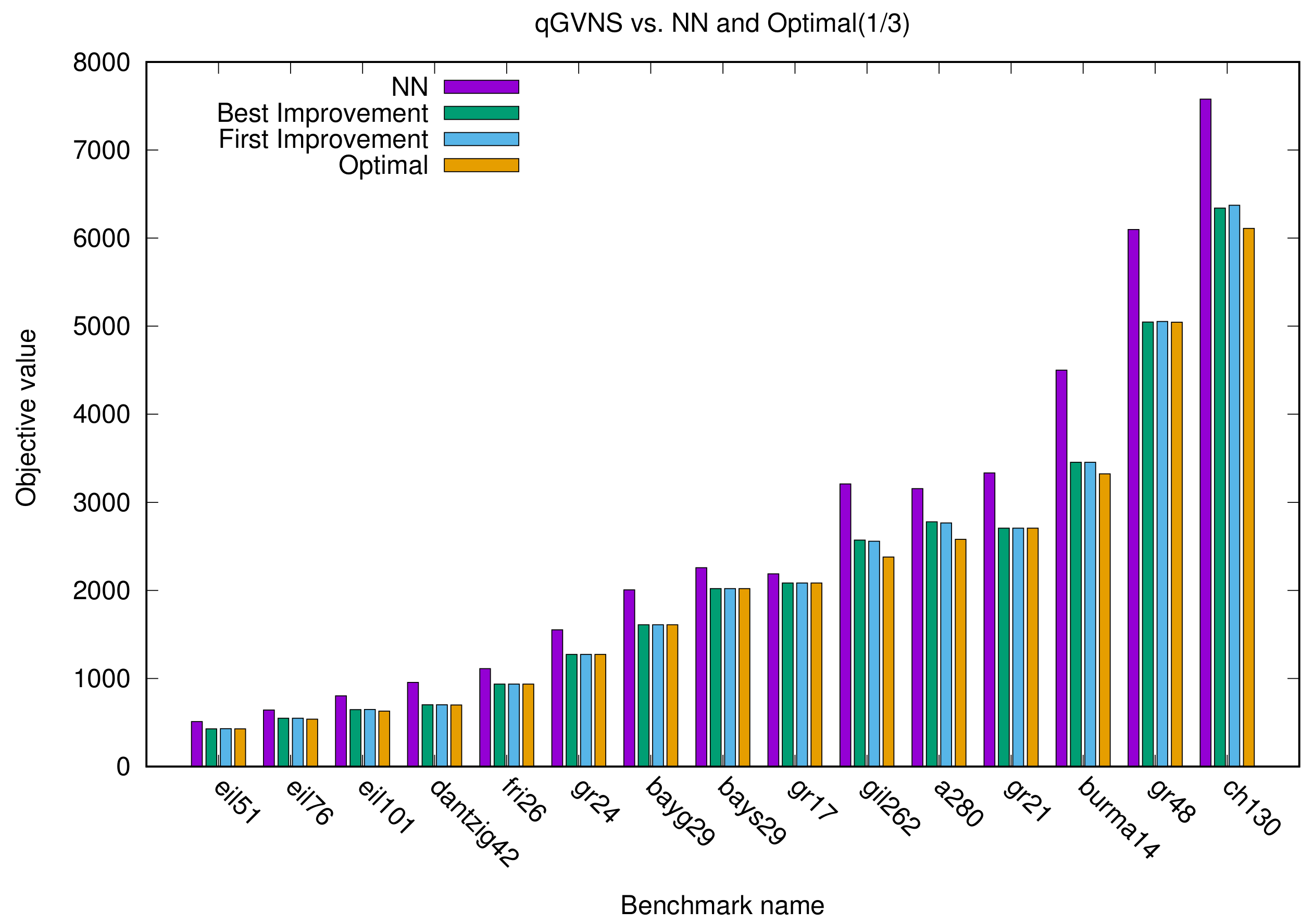
In this section, we present two different sets of figures with three different bar charts for each set. Each figure concerns a different subset of the total experiments, sorted according to the optimal value. In the first set (Figure 1, Figure 2 and Figure 3), each benchmark problem is represented with four different bars, one for each method. Specifically, one represents the NN algorithm, one the optimal value, and another two depict GVNS (best and first improvement). It can be easily seen that our implementation achieves results very close to optimal, unlike the NN algorithm, which does not provide efficient solutions.

A notable example of Figure 1 is ch130. We can see that GVNS (using either FI or BI) is much closer to the optimal value, compared to NN.

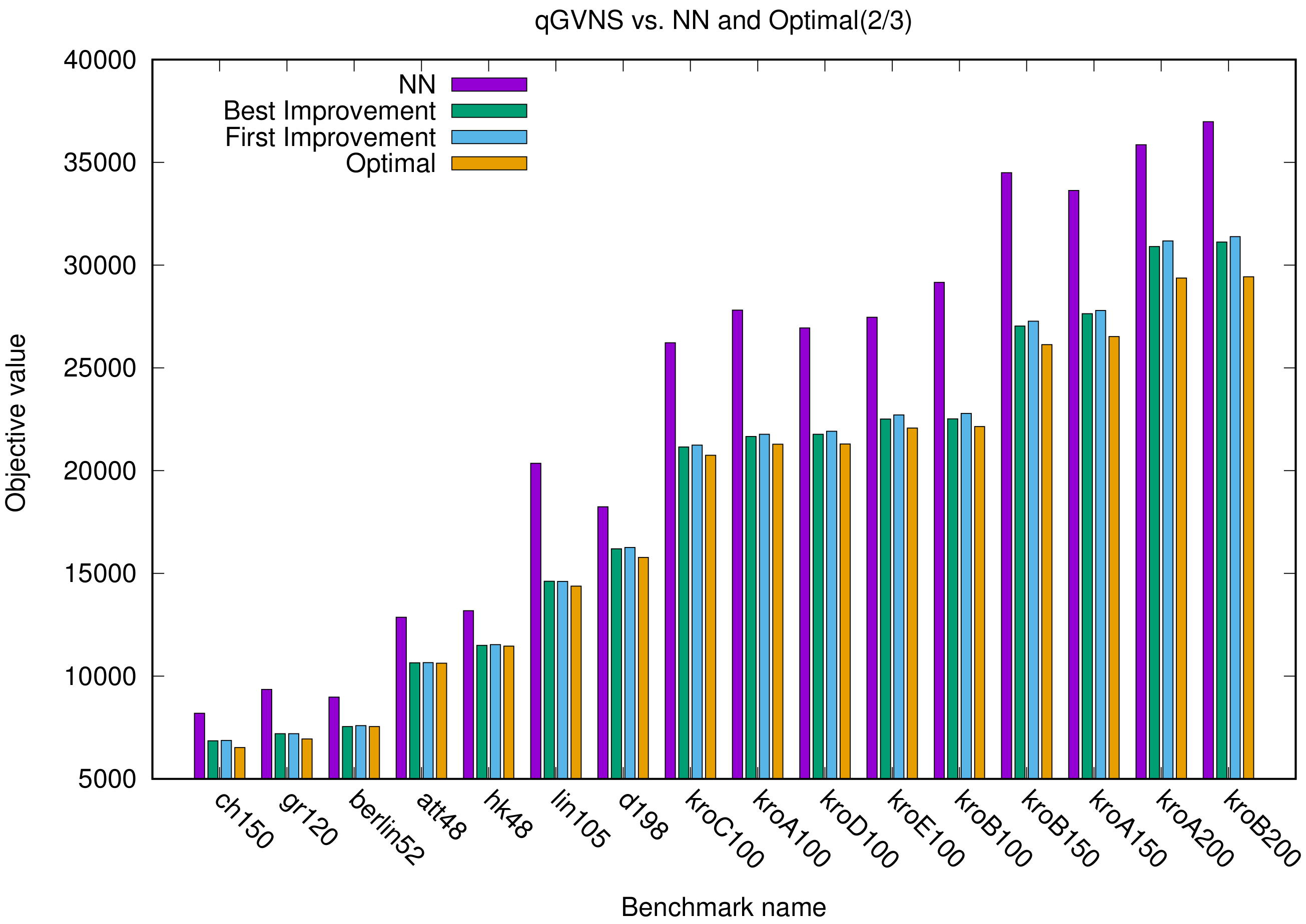
It is clear from Figure 2 that, in kroC100, KroA100, KroD100, KroE100, KroB100, KroB150, KroA150, KroA200, and KroB200, the gap between the NN method and both variants of the GVNS is too high. We can also observe some cases in Figure 2, where the GVNS achieves the optimal value. These are berlin52, hk48, and att48.

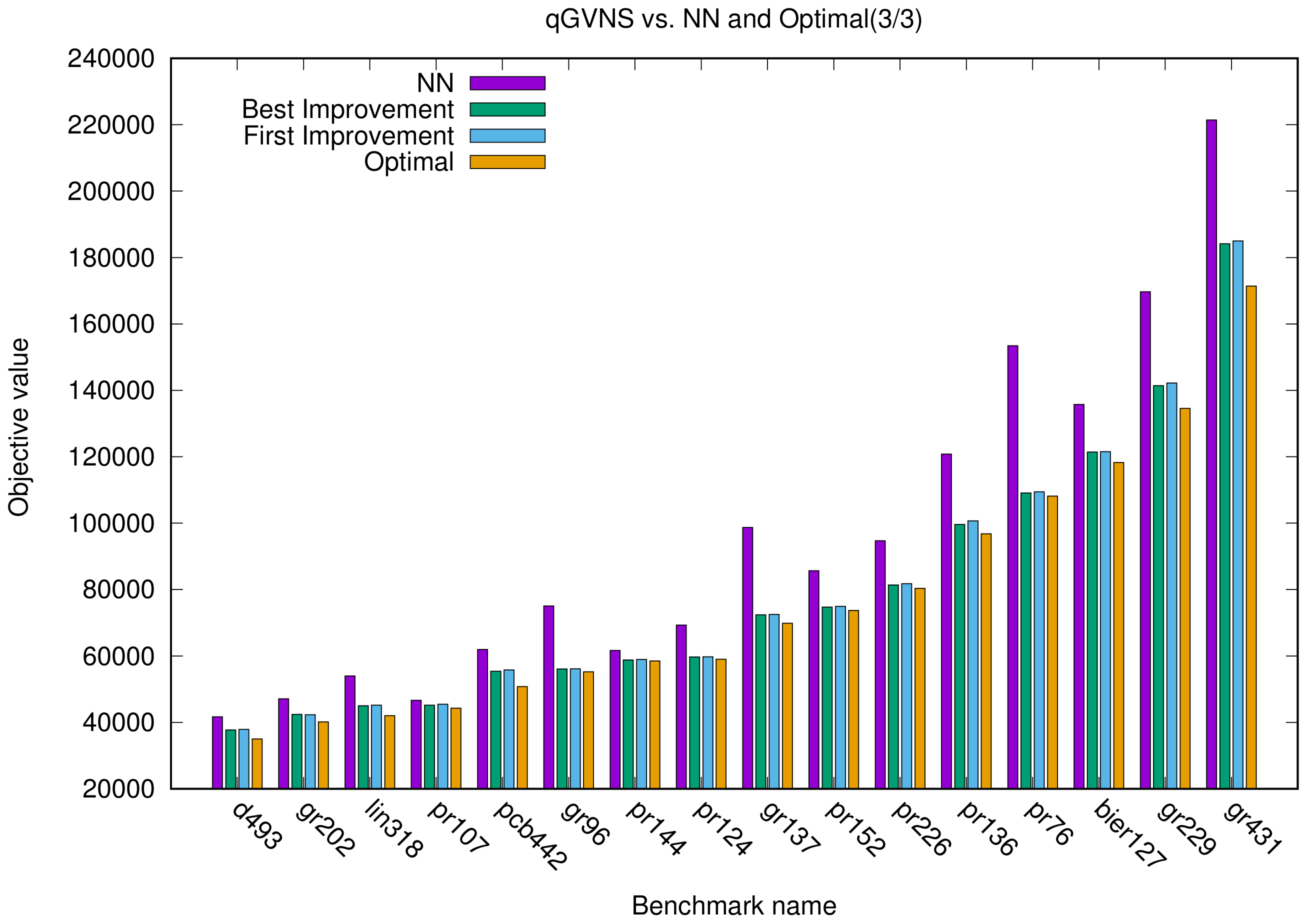
We observe that, in most benchmarks, in Figure 3, GVNS using FI or using BI comes close to the optimal value, while the NN bar is further away from the optimal value. Examples include lin318, pr124, gr137pr76, bier127.

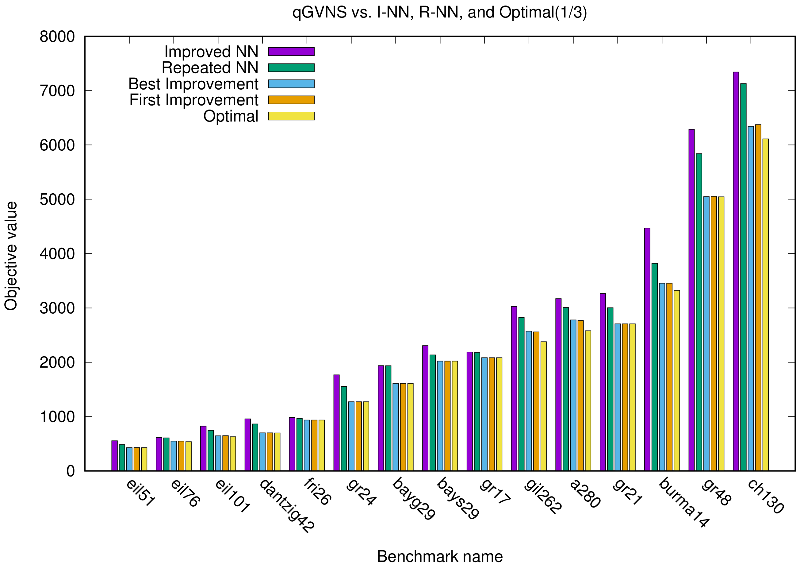
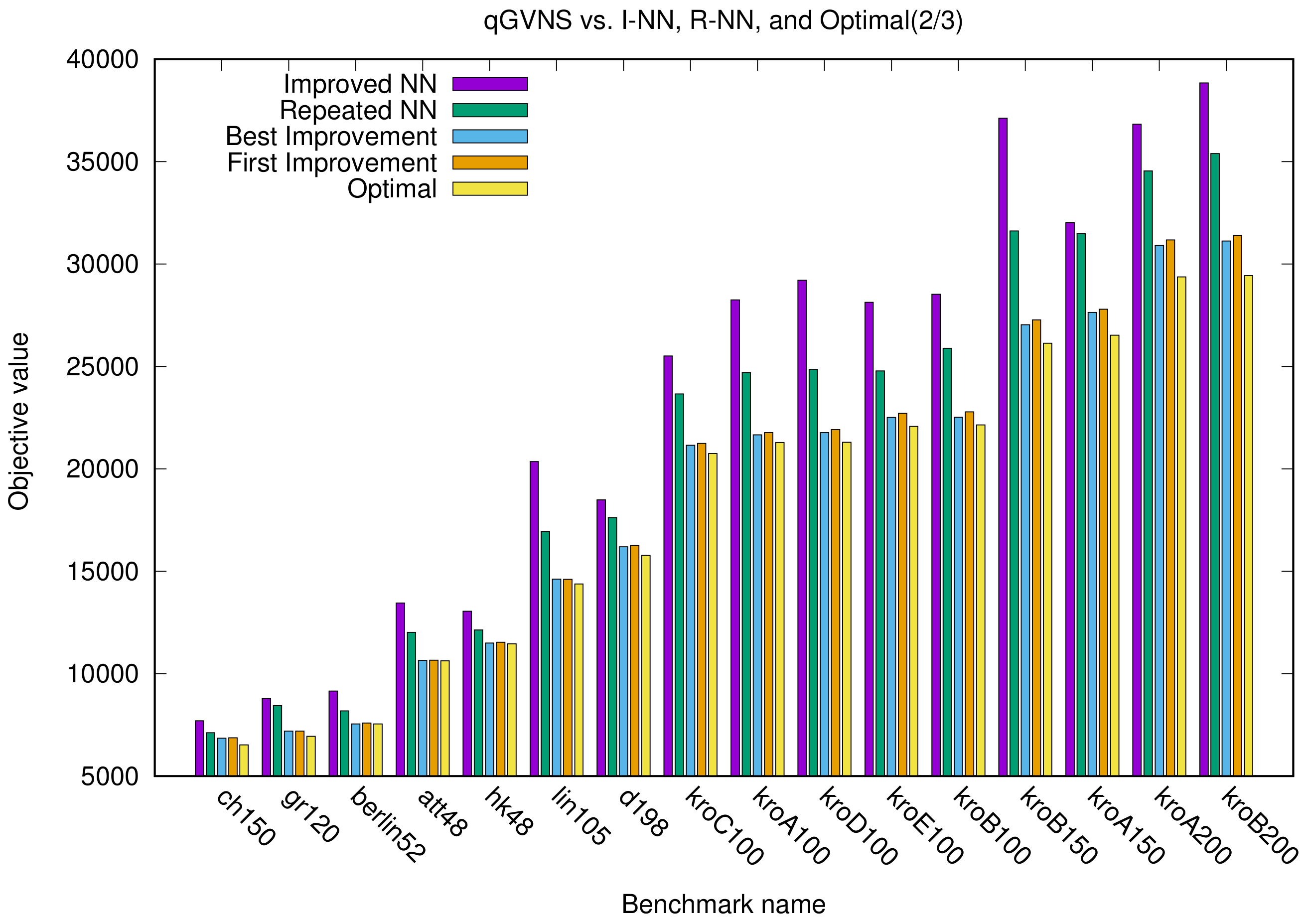
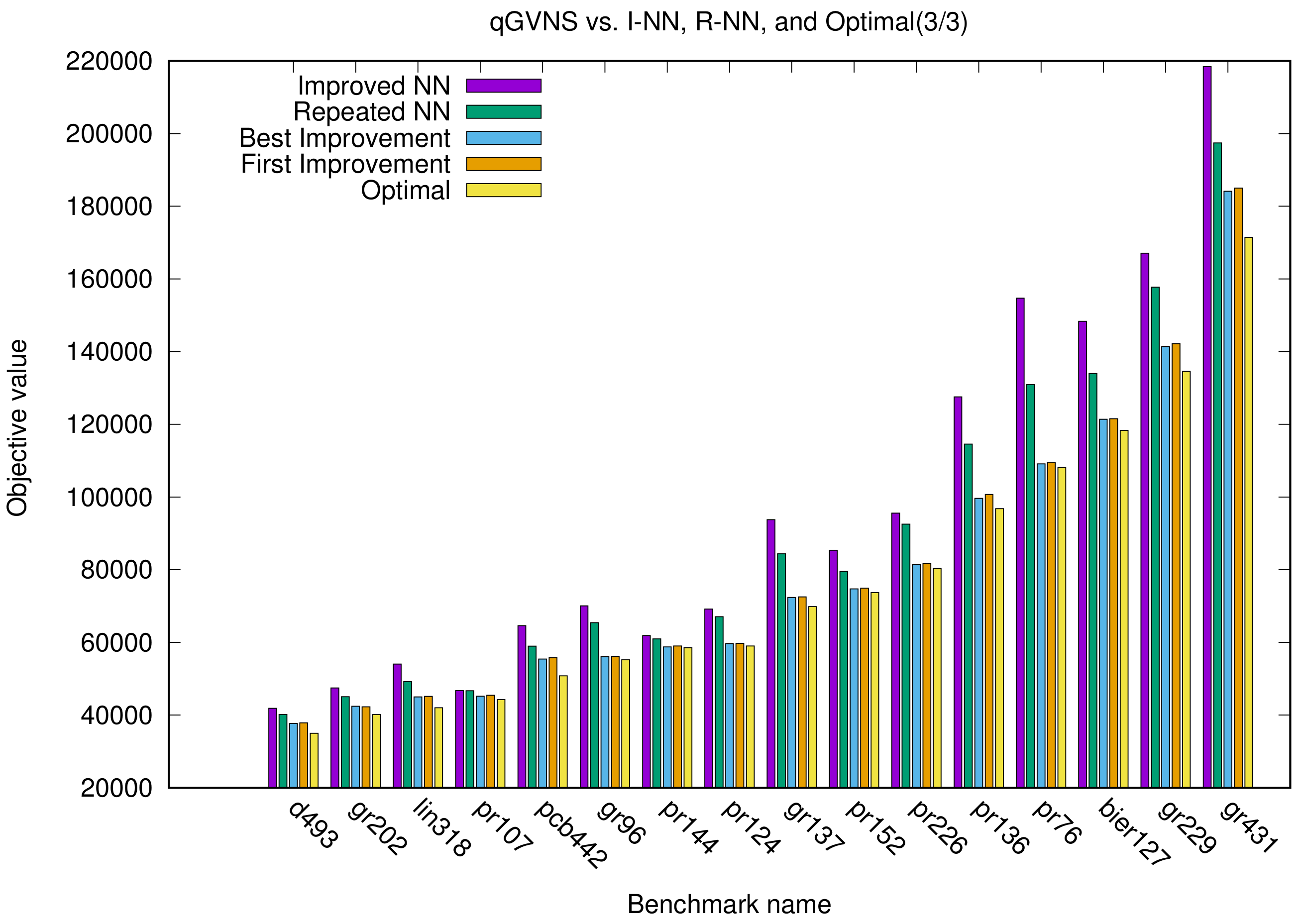
In the next set of figures (i.e., Figure 4, Figure 5 and Figure 6), each benchmark is represented with five different bars; one for the improved NN algorithm, one for the repeated NN algorithm, one for the optimal value, and another two for our implementation (best and first improvement). A close examination reveals that GVNS is once again very close to optimal values, whereas the improved and repeated NN algorithms fail to provide equally good solutions.

Looking at Figure 4, we infer that, when it comes to medium benchmark problems, GVNS significantly approximates the optimal value, unlike both variants of NN, which are far from the optimal. We can particularly see this with kroB100, lin105, kroB150 and kroB200.

In general, Figure 4, Figure 5 and Figure 6 show that the improved NN appears to be a better method than repeated NN. However, in all cases, both GVNS variants outperform the two NN variants.

Figure 6 demonstrates once again the superiority of GVNS. Let us consider benchmark pr76, where GVNS touches the optimal point, while both the repeated and improved NN have a much lower performance. In addition, in Figure 4, Figure 5 and Figure 6, we can see for a different set of benchmarks that again GVNS outperforms the NN variants, significantly closer to the optimal value in each case.

To sum up, the graphical results allow us to conclude that GVNS with BI or FI produces results that are appreciably close to the OV in most benchmark tests, whereas the NN algorithm is far from being close (for every case). Previously, we provided the analytical results in tabular form. The graphical representation of these results makes it easy to see the efficiency of the proposed algorithm, since one can immediately see that the divergence from optimal is almost negligible.

6. Conclusions and Future Work

This work studied an application of garbage collector routing using a new metaheuristic method based on a novel version of GVNS. We modeled the underlying problem as a TSP instance and went on to solve it using GVNS. Our GVNS algorithm, differs from conventional approaches due to its inspiration from principles of quantum computing. Our study was focused on quick and efficient transitions to different areas of the search space. This enabled us to find efficient routes in a short period of time. To assess the efficiency of our approach, we performed extensive experimental tests using well-known benchmarks from TSPLIB. The results were quite encouraging, as they confirmed that the novel GVNS outperforms methods that are widely used in practice, such as NN, repeated NN, and improved NN.

A direction for future work could be the investigation of alternative neighborhood structures and neighborhood change moves in VND (variable neighborhood descent) under the GVNS framework. In the same vein, one could study modifications during the perturbation phase in order to achieve even closer to optimal solutions, particularly on bigger asymmetric benchmarks. Yet another direction could be the use of a multi-improvement strategy [43]. In any event, we plan to apply, adopt if necessary, and assess GVNS to other TSP variants and real-life routing optimization problems.