An Approach for Setting Parameters for Two-Degree-of-Freedom PID Controllers


1
School of Mechanical Engineering, University of Science and Technology Beijing, Beijing 100083, China
2
State Key Lab of Power Systems, Department of Thermal Engineering, Tsinghua University, Beijing 100084, China
3
Key Lab of Energy Thermal Conversion and Control of Ministry of Education, Southeast University, Nanjing 210096, China
*
Author to whom correspondence should be addressed.
Algorithms 2018, 11(4), 48; https://doi.org/10.3390/a11040048
Submission received: 19 March 2018
/
Revised: 5 April 2018
/
Accepted: 6 April 2018
/
Published: 13 April 2018
(This article belongs to the Special Issue Algorithms for PID Controller)
Abstract
:In this paper, a new tuning method is proposed, based on the desired dynamics equation (DDE) and the generalized frequency method (GFM), for a two-degree-of-freedom proportional-integral-derivative (PID) controller. The DDE method builds a quantitative relationship between the performance and the two-degree-of-freedom PID controller parameters and guarantees the desired dynamic, but it cannot guarantee the stability margin. So, we have developed the proposed tuning method, which guarantees not only the desired dynamic but also the stability margin. Based on the DDE and the GFM, several simple formulas are deduced to calculate directly the controller parameters. In addition, it performs almost no overshooting setpoint response. Compared with Panagopoulos’ method, the proposed methodology is proven to be effective.
1. Introduction
The proportional-integral-derivative (PID) controller, which is by far the most common control algorithm, is widely used in the industry due to its simplicity and ease of tuning [1,2]. It is well-known that PID controllers can be implemented in two forms: single-degree-of-freedom (1-DOF) PID and two-degree-of-freedom (2-DOF) [3]. Because the design of the control system can be seen as a multi-objective optimization [4], and because there is a trade-off between the setpoint response and the load disturbance attenuation in the 1-DOF PID structure [5,6], the 2-DOF PID structure was proposed [7]. Due to its superiority, the 2-DOF PID has drawn great attention from many researchers, and a great number of tuning methods have been proposed, such as the dominant poles method [8,9], the internal model control (IMC) [10,11,12], the gain–phase margin method (GPM) [13], the maximum sensitivity method [14,15], the desired dynamic equation method (DDE) [16,17,18], etc.
The tuning method proposed is an improvement of the DDE method. The DDE is a 2-DOF tuning method based on the desired dynamic, disturbance estimate, and disturbance compensation. The DDE method has the following advantages. On the one hand, it endows the controller parameters with physical meanings [19,20], because it can build the equivalent relationship between the 2-DOF PID structure and the Tornambe controller (TC) [21] structure, which is characterized by clear physical meanings. On the other hand, due to the equivalent relationship between the 2-DOF PID structure and the TC, the DDE makes the parameter settings of the 2-DOF PID not dependent on a precise model [22,23]. The nature of the TC is that a disturbance observer estimates the total disturbance and then dynamically compensates it; therefore, the model error can be seen as an internal disturbance that is estimated and then compensated. However, the major drawback of the DDE method is that the stability margin cannot be guaranteed. So, we propose using the generalized frequency method (GFM) in addition to the DDE method, because this DDE–GFM can guarantee both the desired dynamic and the stability margin [24].
The GFM can guarantee the stability margin by limiting the closed-loop poles to a stability sector area in the left half-plane. What is more, it can not only accurately guarantee the specified stability margin by only one parameter but also calculate the controller parameter directly and analytically, whereas (the maximum sensitivity) and GPM cannot realize these two purposes simultaneously. In addition, the GFM has been used to set single-degree-of-freedom PID parameters [25]. Thus, the GFM has been chosen to be the stability margin criterion.
In [24,25], the GFM builds the relationship between the controller parameters and the stability margin. Moreover, it is known that the DDE method builds the relationship between the 2-DOF PID and the TC, and the TC builds the relationship between the controller parameters and the desired dynamic. So, the desired dynamic, represented as the controller parameters and , and the stability margin, represented as the controller parameter , can be specified. Then, a contour, characterized by the same , , and , is obtained. In the contour, an appropriate work point is derived to calculate the controller parameters. Finally, an appropriate work point to calculate the controller parameters can be obtained. This is the principle of the DDE–GFM.
The tuning steps of the DDE–GFM are briefly shown as follows. It is known that the parameters of the 2-DOF PID have been converted into the parameters of the TC according to the DDE. Firstly, , , and are specified based on the desired dynamic and the stability margin, then and are converted into and . Next, the contour is depicted in the plane, restraining the stability margin with the GFM. Finally, an appropriate work point is derived, which possesses a big enough to improve the estimation of the total disturbance to calculate the controller parameters.
The proposed method not only guarantees the desired dynamic but also the stability margin. Moreover, several simple formulas were deduced to calculate directly the controller parameters. In addition, it performs almost no overshooting setpoint response because the desired dynamic is in critically damped system. Compared with Panagopoulos’ method [15], the settling time is shortened and the overshooting is drastically decreased, while the maximum sensitivity stays the same.
This paper is organized as follows. Section 2 describes the related tuning methods (i.e., the desired dynamics equation method and the generalized frequency method) and the steps of setting the controller parameters. Section 3 offers some examples with simulations to illustrate the analysis of the controller parameters in detail. A comparison with Panagopoulos’ method is also included in this section. Section 4 is the conclusion.
2. The Related Tuning Methods
2.1. The Desired Dynamics Equation (DDE) Method
Consider the transfer function given by:
where and are unknown parameters. It can be transformed to the following state space form:
where are the plant input and its derivatives; is the plant output; are the system states; is a proper positive constant number; and is the total disturbance.
The desired dynamic equation is as follows:
To reach Equation (3), the corresponding control law should be:
where and are the coefficient of the desired dynamic and are determined by the requirements of the control system; and is the estimation of total disturbance .
To obtain the estimation of total disturbance , the following disturbance observer is used.
where is the coefficient of the disturbance observer and indicates the speed of tracking disturbance; and is an intermediate variable.
Equation (5) structures a disturbance observer. Equation (4) offers the control law to achieve the desired dynamic Equation (3). The disturbance observer estimates the total disturbance and compensates the systems to be the desired dynamic in real time and dynamically.
By substituting Equations (2), (3) and (5) into Equation (4), we can obtain
where is the target value; and is the error between the plant output and the target value. The detailed derivation is shown in Appendix A.
From Equation (6), we can obtain the two-degree-of-freedom PID controller parameters,
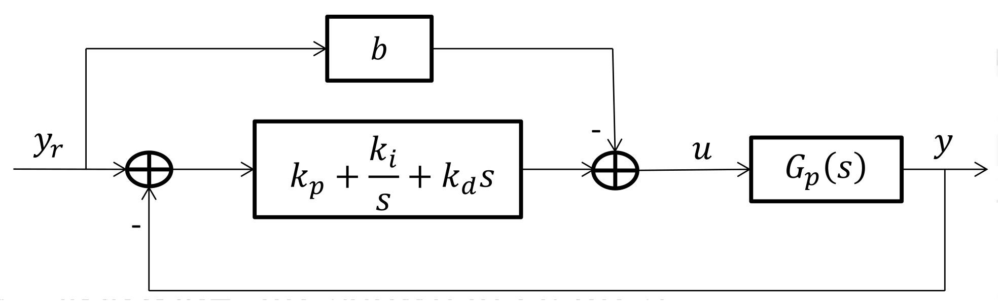
The corresponding two-degree-of-freedom PID controller structure is shown in Figure 1.
When the desired dynamic equation is as follows:
we can analogously obtain the two-degree-of-freedom PID controller parameters,
In general, the DDE endows the 2-DOF PID controller parameters with clear physical meaning, which makes some of the parameters specified and then decreases the number of unknown parameters. Moreover, the model error is imposed into the total disturbance and is compensated, so the precise model is not necessary.
2.2. Generalized Frequency Method (GFM)
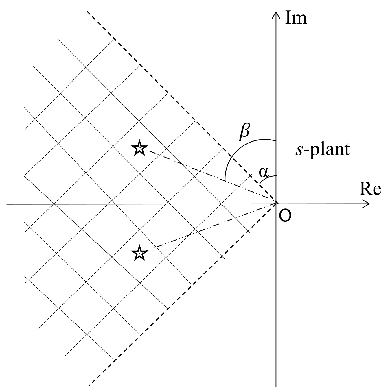
The GFM can calculate the controller parameters directly and analytically and can accurately guarantee the specified stability margin with only one parameter, which is called the attenuation index . The attenuation index determines the two rays, which shape a sector area shown in Figure 2, and the GFM can make all the closed-loop poles lie in the resulting sector area. The equation of the two rays is , where , . is a constant and is the included angle between the ray and the imaginary axis.
The stability margin increases with attenuation index . Each pair of conjugate complex poles have a corresponding , and the corresponding equal to infinity for the real poles. The minimum is equal to the specified attenuation index , i.e., .
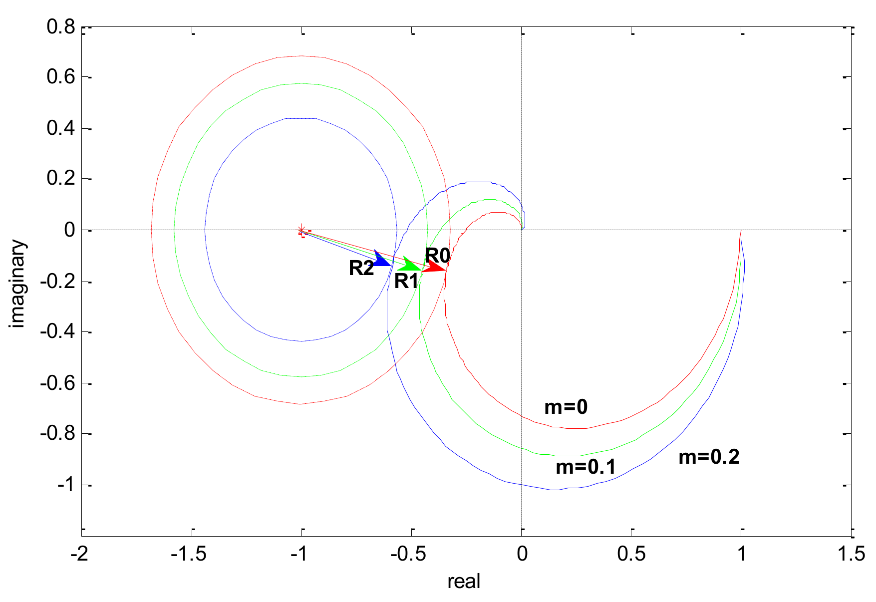
Next, we will illustrate the relationship between the maximum sensitivity () and the attenuation index to explain the rationality of the attenuation index as the stability margin criterion. is taken as an example. Substitute into , and the Nyquist plots of are shown in Figure 3.
In Figure 3, the Nyquist plots are shown with full lines, and , , and are respectively shown with a red line, green line, and blue line; dashed lines represent the maximum sensitivity and the dashed red line, green line, and blue line respectively represent , , and . The stability margin of decreases with the attenuation index increasing. So, when designing the controller parameters, make the transfer function to give as the stability margin, where represents the transfer function of the controller. From above, the attenuation index can give a system stability margin in parameter design stage, and thus, it can be a stability margin criterion.
2.3. Setting PID Controllers Parameters
In this subsection, first a set of tuning equations is derived, and then, controller parameters are analyzed. Finally, the steps of the tuning method are given.
For the control system in Figure 1, its stability is determined by the closed-loop characteristic equation:
Substitute into Equation (10), define , and compare the real and imaginary parts; the following equation is obtained
Under certain , Equation (11) structures a marginal stability surface with various . The marginal stability surface divides the space into two parts: meeting stability margin and not meeting stability margin.
Employing the following variable substitution,
Equation (7) is expressed as
Substitute Equation (13) into Equation (11), and the following equation is obtained
Under certain , , and , Equation (14) becomes a linear equation. Then, if its Jacobian determinant J is nonsingular, it has a unique local solution . Under various and certain , and , Equation (14) has a unique local solution curve (i.e., marginal stability curve). The marginal stability curve divides the plane into two parts: meeting stability margin and not meeting stability margin. The curve is the contour. Then, once an appropriate work point in the contour is obtained, the controller parameters can be calculated. The method of choosing a work point is shown after the analysis of the parameter , because the parameter can influence the choosing method.
Next, the function of the controller parameters is analyzed, and the method for obtaining them is shown.
and are coefficients of the desired dynamic equation. They are chosen based on the requirements of control system, such as settling time, overshooting, and so on. Because the desired dynamic equation is a second-order system, and can be calculated according to the second-order system, as follows:
where is the desired settling time; is the damping of desired dynamic system; and is the natural frequency of desired dynamic system.
In order to make the overshooting as small as possible and make the settling time as short as possible, is chosen. Considering the error between the actual dynamic and the desired dynamic, Equation (15) becomes
The stability margin increases with the increasing of the attenuation index . It is well-known that there is a trade-off between performance and robustness [26,27]. Therefore, choosing an appropriate is important to avoid the conflict with both and . According to our experience, the reasonable selecting region of is generally . One other thing to note is that a greater is needed when the model is imprecise.
Combine Equation (2) with Equation (5) and do a Laplace transform, and the following equation is obtained:
Its derivation is shown in Appendix B.
As shown in Equation (17), the response rate of the disturbance observer speeds up with increasing. So, the work point should be chosen nearby the q-axis in order to make as large as possible because in the plane.
The work point is chosen as follows.
First, substitute into Equation (14), and the following equation is obtained.
Solve Equation (18), and and can be obtained.
Then, define
and substitute into Equation (14), so and can be obtained. The point is the work point in the plane.
Finally, substitute and into Equation (13), and the controller parameters are obtained.
The steps of setting the controller parameters are shown as follows:
- (1)
- Obtain the system model and choose proper , and values according to the requirements of system;
- (2)
- Solve Equation (18), and then get and ;
- (3)
- Get from Equation (19), substitute into Equation (14), and then get and ;
- (4)
- Substitute and into Equation (13) to calculate the controller parameters. If there are closed-loop poles outside of the sector area, decrease both and simultaneously or only , and then turn to step (2); otherwise, continue;
- (5)
- Do the step response and calculate the settling time and overshooting. If the settling time is not met, then increase both and or decrease , and turn to step (2); if the overshooting is too great, then decrease both and or increase , and turn to step (2); otherwise, continue;
- (6)
- End.
3. Illustrative Examples
To demonstrate the application of the 2DOF PID tuning method proposed in the previous sections, now the simulation results for different processes are presented using MATLAB. In this section, firstly the previous theoretical analysis of the controller parameters is verified with simulation. Then, compared with Panagopoulos’ method [15], the proposed method is effective and superior.
3.1. PID Controller Parameters Analysis with Simulation
In this subsection, the influence of the controller parameters will be analyzed through simulation.
Consider a process given by .
If the settling time is less than 10 s, the desired dynamic coefficient can be calculated from Equation (16). and are chosen. The contours are shown in Figure 4 where is equal to 0.5, 0.6, 0.7, and 0.8 respectively.
As shown in Figure 4, the greater the , the closer to origin the contour. Parameter increases in the counter-clockwise direction. In order to analyze the influence of parameter and parameter on the behavior of the closed-loop time response and the frequency response, seven points A, B, C, D, E, F, and G are chosen. Among them, points C, D, E, and F are characterized by the same stability margin , and points A, B, C and G are characterized by roughly the same disturbance observer coefficient , which is big enough. The coordinates of the seven points in the plane are listed in Table 1.
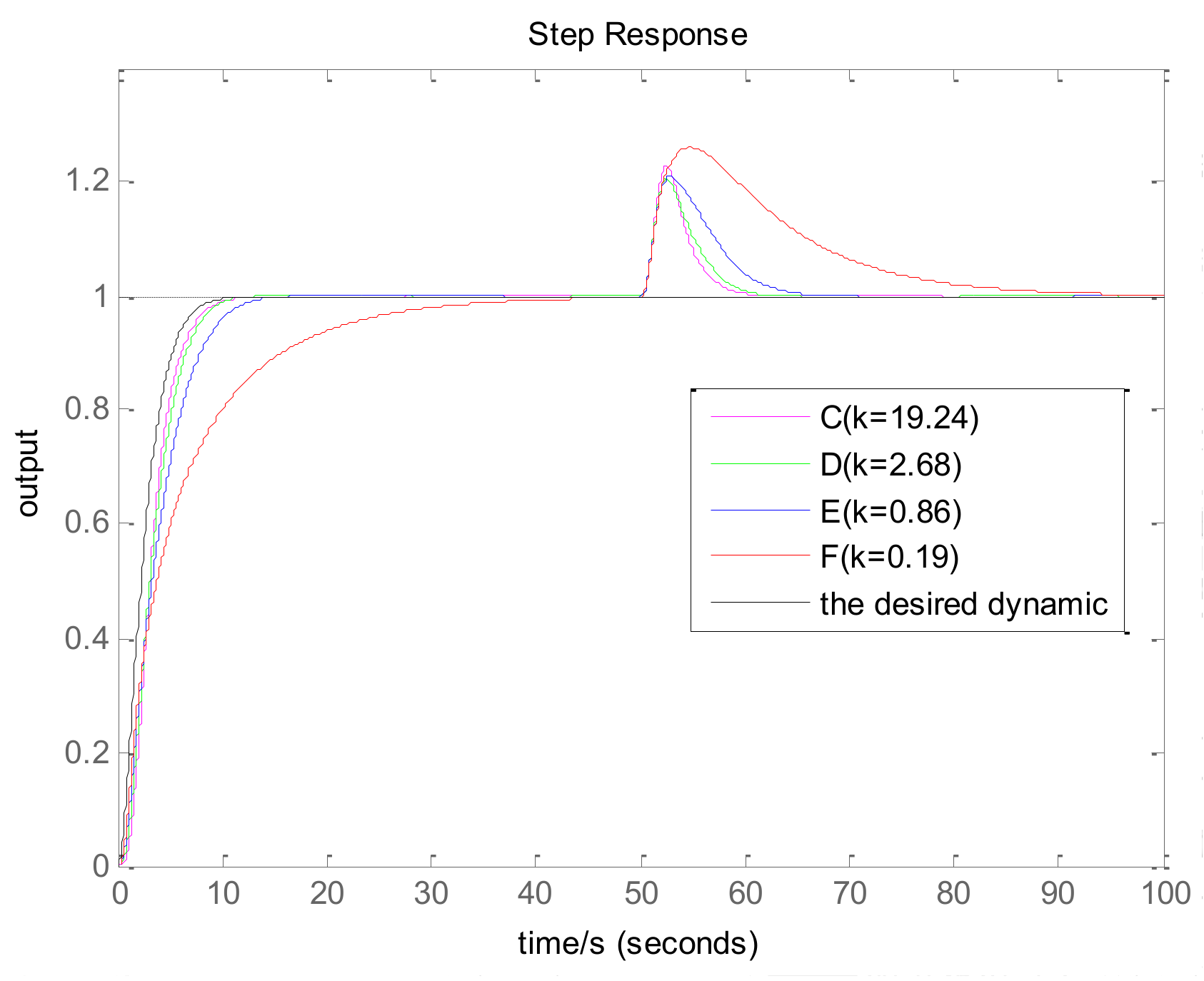
The closed-loop time response and the closed-loop frequency response of process for points C, D, E, and F are shown in Figure 5, Figure 6 and Figure 7, which show the influence of parameter . In the time response case, load disturbance is introduced at t = 50 s.
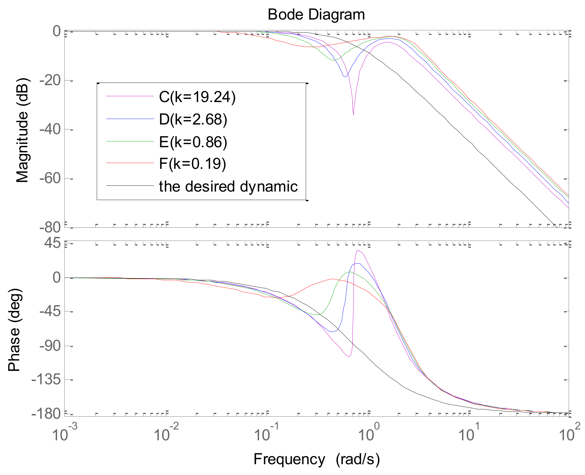
On the one hand, from the simulation results of Figure 5, it can be observed that the setpoint response is closer to the desired dynamic with the increasing . Furthermore, the influence of is weakened when adds up to certain values that are too great. In Figure 6, the frequency characteristic of the low-frequency range is closer to the desired dynamic with the increasing . On the other hand, in Figure 5, the load disturbance response is also improved with the increasing . The reason is that the integral coefficient enlarges with the increasing . In addition, the influence of is weakened when adds up to certain high values. In Figure 7, the amplitude of the low-frequency range is lower with the increasing .
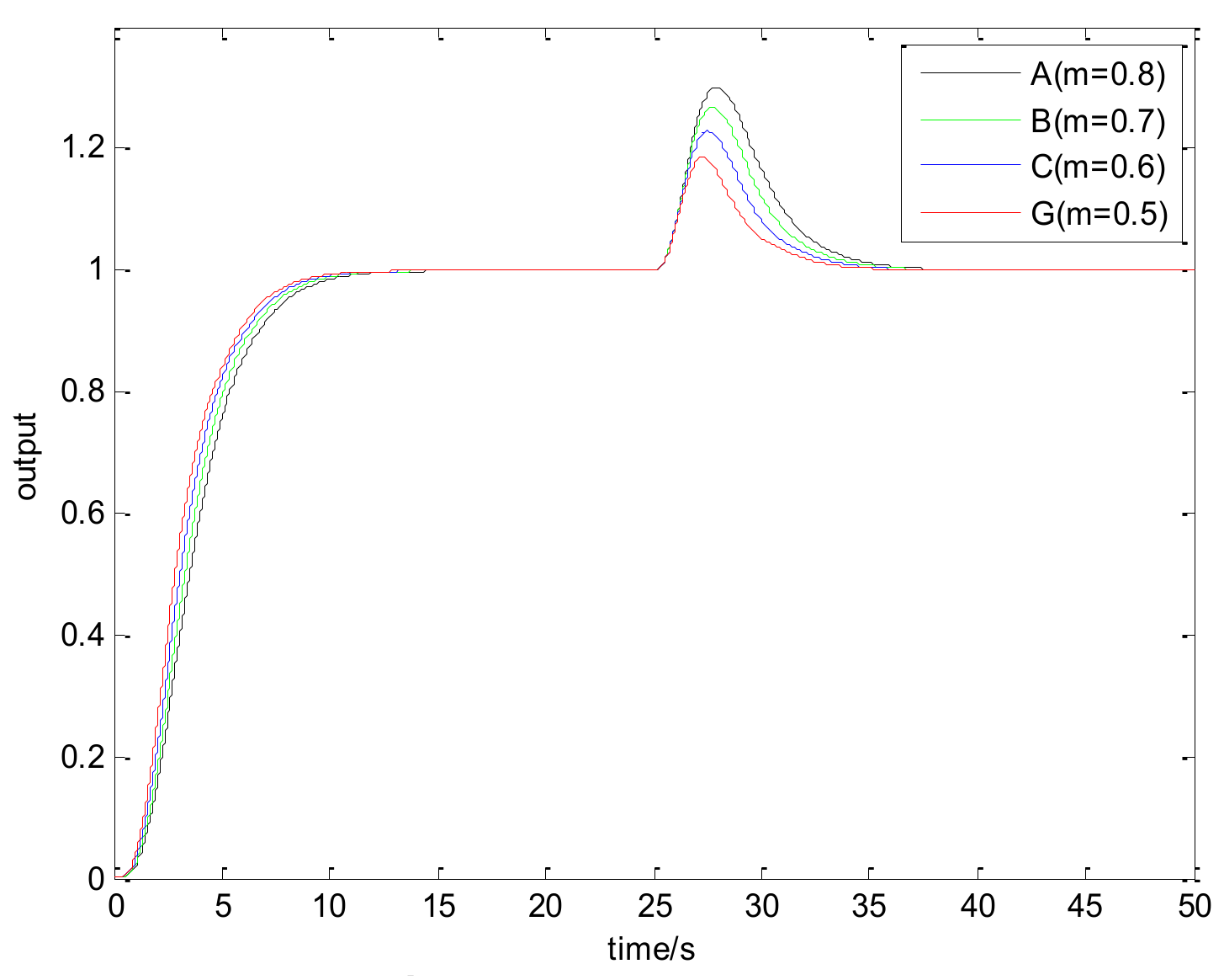
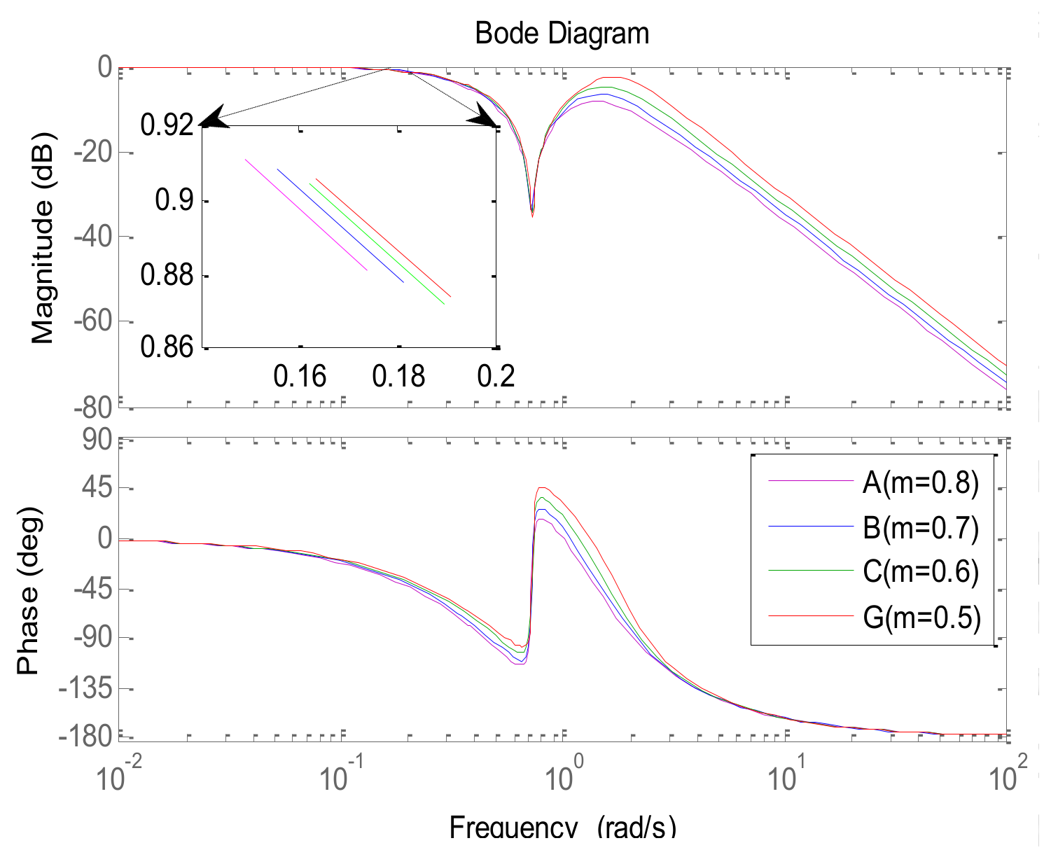
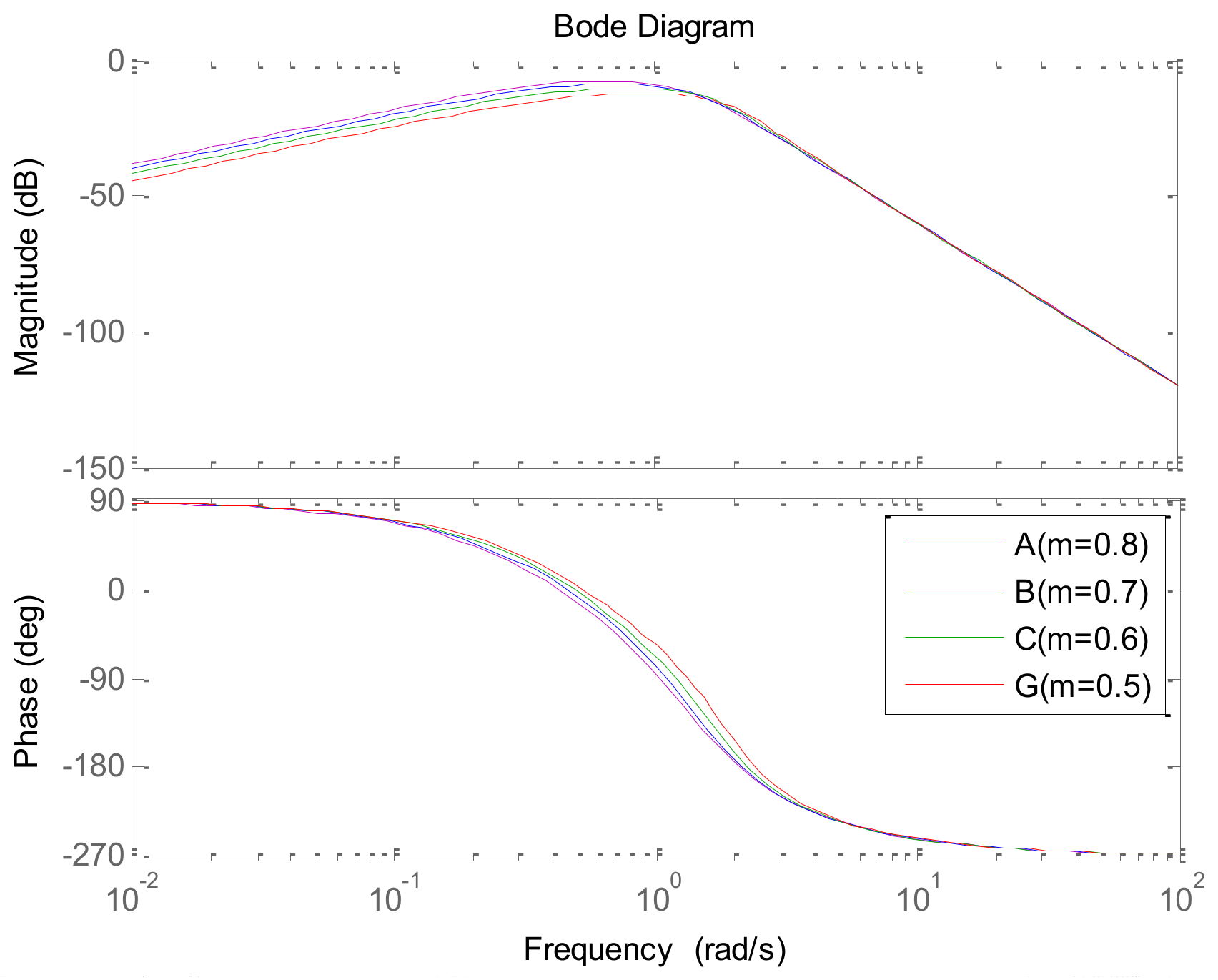
The closed-loop time response and the closed-loop frequency response of process for points A, B, C, and G are shown in Figure 8, Figure 9 and Figure 10 from which the influence of parameter can be seen. In the time response case, the load disturbance is introduced at t = 25 s.
On the one hand, in Figure 8, the setpoint response rate is slower with the increasing . In Figure 9, the magnitude of the low-frequency range is also closer to 0 dB. On the other hand, in Figure 8, the load disturbance response is deteriorated with the increasing . In Figure 10, it is shown that the magnitude of the low-frequency range is higher with a greater . The above phenomena are a result of the stability margin increasing with the increasing , and there is a trade-off between performance and robustness.
To demonstrate the influence of and , the same and = different are chosen, and then, the contours are depicted in Figure 11 where and are respectively equal to , , and .
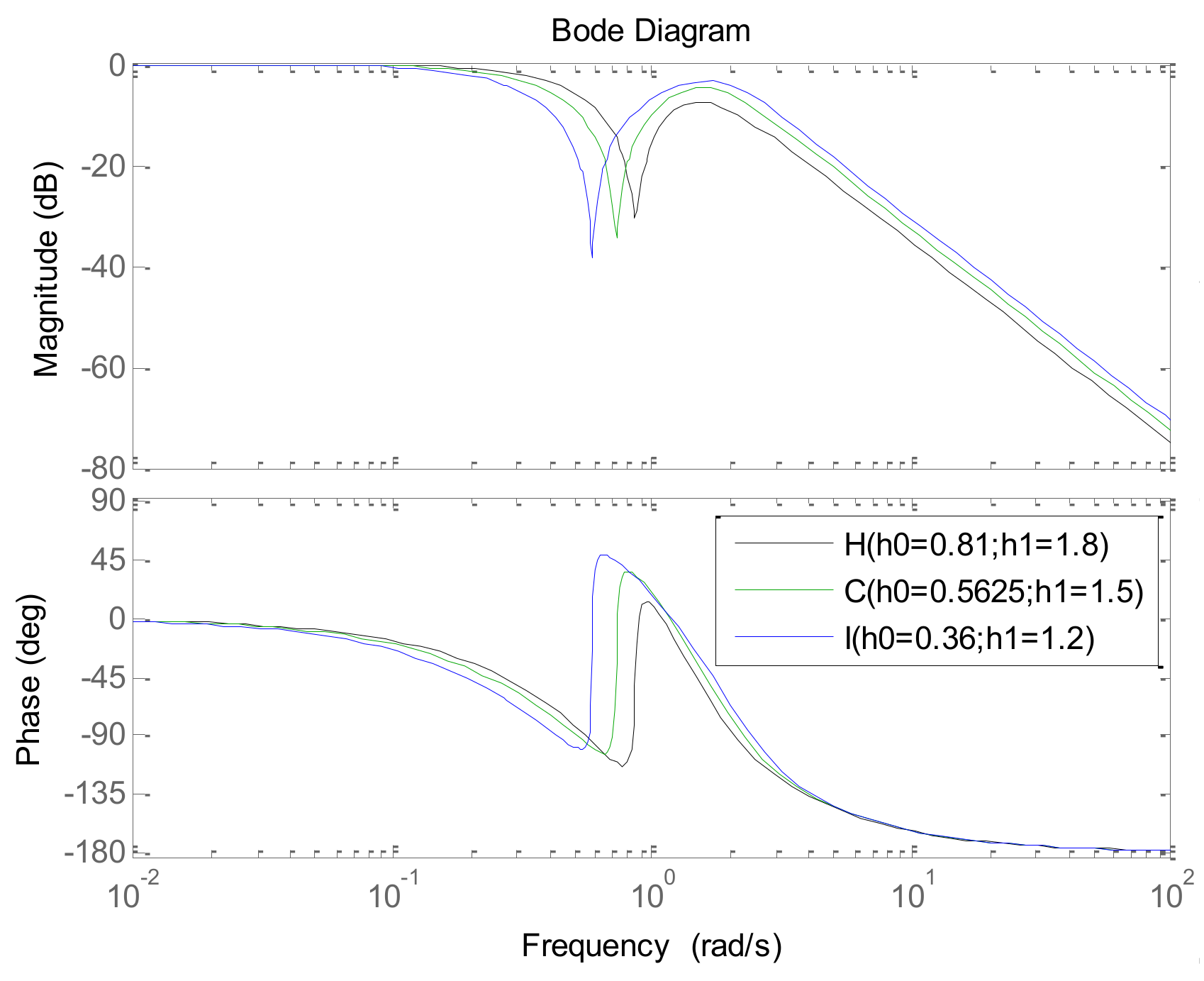
As shown in Figure 11, the contour is closer to the origin with the increasing of both and . To analyze the influence of both and , three points H, C, and I were chosen. The coordinates of these points in the plane are listed in Table 2.
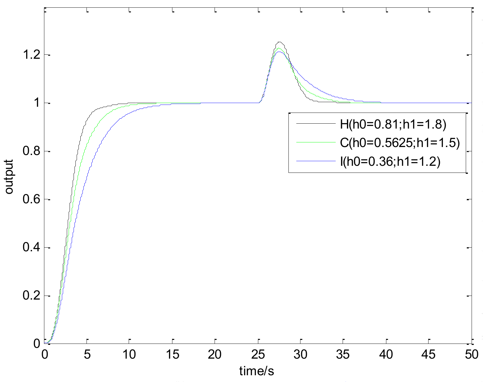
The closed-loop time response and the closed-loop frequency response of process for points H, C, and I are shown in Figure 12 and Figure 13, which show the influence of the parameters and . In the time response case, the load disturbance is introduced at t = 25 s.
On the one hand, Figure 12 shows that the setpoint time response speeds up by increasing both and . From Figure 13, it can be observed that the magnitude of the low-frequency range is closer to 0 dB. The above phenomena result from the fact that the desired dynamic is faster with greater and . On the other hand, Figure 12 also shows that the load disturbance response returns to the target faster, and the peak is higher with greater and .
The simulation results of the nine points A~I have not only shown the influence of the parameters , but also prove that the specified stability margin can be met as follows. All the closed-loop poles of points from A to I are shown in Table 3, and it can be seen that all the closed-loop poles lie in the specified sector region. From Table 3, it can be also observed that among all the corresponding to the poles, the smallest is equal to the previous specified .
3.2. Comparison with Panagopoulos’ Method
This section will present the results compared with Panagopoulos’ method [15] to show the superiority of the proposed tuning method.
The control law of Panagopoulos’ method is as follows:
Under the condition that , eight different processes [15] serve as examples. The eight processes cover high–order process, non–minimum phase process, time–delay process, and integrating process, which are listed as follows:
Table 4 collects the related parameters of the DDE−GFM, including , , , , , , and , and the related parameters of Panagopoulos’ method, which covers , , , and .
Table 5 presents the position of the work point in the plane of the DDE−GFM and the control signal and time response of the two methods. On the one hand, it can be seen that the work points of all the processes are positive, as well as the nearby q−axis, which can make parameter large enough. Consequently, the estimation of the total disturbance is more precise. On the other hand, the settling time of the DDE−GFM for and is obviously shorter than that of Panagopoulos’ method. Moreover, compared with Panagopoulos’ method, the overshooting of the DDE−GFM is substantially smaller, except for for which the overshooting is zero.
Further details of the simulation results can be seen in Table 6, which includes the settling time, the overshooting, the integral absolute error (IAE), and the maximum sensitivity of the two methods. It can be seen that the settling time is shortened by 15~60%. Except for for which the overshooting is zero, the overshooting of the other processes are all reduced by more than 70%. Furthermore, the overshooting of , , and are even directly reduced to zero. The IAE index of the two methods for each process are approximately equal except for that of for which the IAE index is approximately zero. In addition, the maximum sensitivity of two methods for all the processes are equal to 2.
4. Conclusions
A new tuning method is proposed for a two-degree-of-freedom PID controller, which combines the advantages of the DDE and the GFM. Firstly, choose appropriate , , and . Secondly, calculate using Equation (18). Thirdly, calculate using Equation (19), and then substitute into Equation (14) to calculate . Finally, substitute into Equation (13), and then, calculate the controller parameters. The main advantage of the proposed method is that the desired dynamic and the stability margin can be guaranteed simultaneously. In addition, a set of formulas were obtained to calculate the controller parameters. Moreover, the method can perform a fast setpoint response with minimal overshooting. Compared with Panagopoulos’ method, the proposed method is more effective and superior.
Acknowledgments
National Key Technology Support Program (2015BAF30B00)
Author Contributions
“Donghai Li and Xiaoqiang Yan conceived and designed the experiments; Xinxin Wang performed the experiments; Xinxin Wang and Li Sun analyzed the data; Li Sun contributed reagents/materials/analysis tools; Xinxin Wang wrote the paper.”
Conflicts of Interest
The authors declare no conflict of interest.
Appendix A
From Equation (5), the following equation is obtained:
Substitute into Equation (4), and the following equation is obtained:
Compare Equation (A1) with Equation (A2); the following equation is obtained:
Integrate Equation (A3), and the following equation is obtained:
Substitute Equation (A4) into Equation (A2), and define ; the following equation is obtained:
Appendix B
Take the derivative of the first equation in Equation (5), and the following equation is obtained:
Substitute the second equation in Equation (5) and the second equation in Equation (2) into Equation (A6), and the following equation is obtained:
Substitute the second equation in Equation (5) into Equation (A7), and the following equation is obtained:
Take the Laplace transform of Equation (A8), and the following equation is obtained:
References
- Astrom, K.J.; Hagglund, T. The future of PID control. Control Eng. Pract. 2001, 9, 1163–1175. [Google Scholar] [CrossRef]
- Ang, K.H.; Chong, G.; Li, Y. PID control system analysis, design, and technology. IEEE Trans. Control Syst. Technol. 2005, 13, 559–576. [Google Scholar]
- Åström, K.J.; Hägglund, T. Advanced PID Control; ISA, Research Triangle Park: Durham, NC, USA, 2006. [Google Scholar]
- Araki, M.; Taguchi, H. Two-degree-of-freedom PID controllers. Int. J. Control Autom. Syst. 2003, 1, 401–411. [Google Scholar]
- Middleton, R.H. Trade-offs in linear control system design. Automatica 1991, 27, 281–292. [Google Scholar] [CrossRef]
- De Moor, B.; David, J.; Vandewalle, J.; de Moor, M.; Berckmans, D. Trade−offs in linear control system design: A practical example. Optim. Control Appl. Methods 1992, 13, 121–144. [Google Scholar] [CrossRef]
- Horowitz, I.M. Synthesis of Feedback Systems; Academic Press: New York, NY, USA, 1963. [Google Scholar]
- Dinca, M.P.; Gheorghe, M.; Galvin, P. Design of a PID controller for a PCR micro reactor. IEEE Trans. Educ. 2009, 52, 116–125. [Google Scholar] [CrossRef]
- Viteckova, M.; Vitecek, A. 2DOF PI and PID controllers tuning. IFAC Proc. Vol. 2010, 43, 343–348. [Google Scholar] [CrossRef]
- Morari, M. Robust Process Control; Prentice Hall: Englewood Cliffs, NJ, USA, 1989. [Google Scholar]
- Sutikno, J.P.; Aziz, B.A.; Yee, C.S.; Mamat, R. A new tuning method for two-degree-of-freedom internal model control under parametric uncertainty. Chin. J. Chem. Eng. 2013, 21, 1030–1037. [Google Scholar] [CrossRef]
- Jin, Q.B.; Liu, Q. Analytical IMC−PID design in terms of performance/robustness tradeoff for integrating processes: From 2-Dof to 1-Dof. J. Process Control 2014, 24, 22–32. [Google Scholar] [CrossRef]
- Xing, Z.; Zhu, Q.; Ding, Y. Two-degree-of-freedom IMC−PID design of missile servo system based on tuning gain and phase margin. J. Harbin Eng. Univ. 2006, 27, 404–407. [Google Scholar]
- Alfaro, V.M.; Vilanova, R.; Arrieta, O. Maximum Sensitivity Based Robust Tuning for Two-Degree-of-Freedom Proportional-Integral Controllers. Ind. Eng. Chem. Res. 2010, 49, 5415–5423. [Google Scholar] [CrossRef]
- Panagopoulos, H.; Astrom, K.J.; Hagglund, T. Design of PID controllers based on constrained optimisation. IEE Proc. Control Theory Appl. 2002, 149, 32–40. [Google Scholar] [CrossRef]
- Wang, W.; Li, D.; Gao, Q.; Wang, C. Two-degrees-of-freedom PID controller tuning method. J. Tsinghua Univ. 2008, 48, 1962–1966. [Google Scholar]
- Weijie, W. The PID Parameter Tuning Method and Its Application in Thermal Control; Tsinghua University: Beijing, China, 2009. [Google Scholar]
- Min, Z. Simulation analysis of PID control system based on desired dynamic equation. In Proceedings of the 2010 8th World Congress on Intelligent Control and Automation (WCICA), Jinan, China, 7–9 July 2010; University of Science and Technology: Beijing, China, 2010. [Google Scholar]
- Li, D.; Xue, Y.; Wang, W.; Sun, L. Decentralized PID controller tuning based on desired dynamic equations. In Proceedings of the 19th World Congress The International Federation of Automatic Control, Cape Town, South Africa, 24–29 August 2014; pp. 5802–5807. [Google Scholar]
- Zhang, Y.; Li, D.; Lao, D. Smith predictor in the DDE application. In Proceedings of the 2012 24th Chinese Control and Decision Conference (CCDC), Taiyuan, China, 23–25 May 2012; pp. 2346–2351. [Google Scholar]
- Tornambe, A.; Valigi, P. Decentralized controller for the robust stabilization of a class of MIMO dynamical systems. J. Dyn. Syst. Meas. Control Trans. ASME 1994, 116, 293–304. [Google Scholar] [CrossRef]
- Hu, Z.; Wang, J.; Li, D.; Qin, J. Application of Desired Dynamic Equation method in simulation of four-tank system. In Proceedings of the 2012 International Conference on Systems and Informatics (ICSAI), Yantai, China, 19–20 May 2012; pp. 366–370. [Google Scholar]
- Hu, Y.; Li, D.; Zhu, M.; Gu, T. Active control of combustion oscillations based on desired dynamic equation. In Proceedings of the 2010 International Conference on Control Automation and Systems (ICCAS), Gyeonggi-do, Korea, 27–30 October 2010; pp. 787–791. [Google Scholar]
- Laijiu, C. Automatic Control Principle and Application for Thermal Process; Water Conservancy and Electric Power Press: Beijing, China, 1982. [Google Scholar]
- Xianyong, Y. Automatic Control for Thermal Process, 2nd ed.; Tsinghua University Press: Beijing, China, 2008. [Google Scholar]
- Alfaro, V.M.; Vilanova, R. Simple robust tuning of 2DoF PID controllers from a performance/robustness trade−off analysis. Asian J. Control 2013, 15, 1700–1713. [Google Scholar] [CrossRef]
- Alfaro, V.M.; Vilanova, R.; Mendez, V.; Lafuente, J. Performance/robustness tradeoff analysis of PI/PID servo and regulatory control systems. In Proceedings of the 2010 IEEE International Conference on Industrial Technology, Vina del Mar, Chile, 14–17 March 2010; pp. 111–116. [Google Scholar]
Figure 1.
Two-degree-of-freedom proportional-integral-derivative (PID) controller structure.

Figure 2.
Generalized frequency characteristic.

Figure 3.
The relation between the maximum sensitivity and the attenuation index m in Nyquist plots.
Figure 3.
The relation between the maximum sensitivity and the attenuation index m in Nyquist plots.

Figure 4.
The contours.
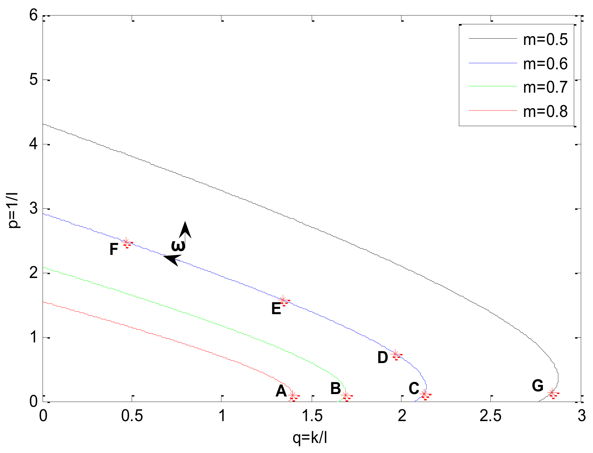
Figure 5.
The time response of process for points C, D, E, and F. Load disturbance is introduced at t = 50 s.
Figure 5.
The time response of process for points C, D, E, and F. Load disturbance is introduced at t = 50 s.

Figure 6.
The closed-loop setpoint frequency response of the process for points C, D, E, and F.

Figure 7.
The closed-loop load disturbance frequency response of the process for points C, D, E, and F.
Figure 7.
The closed-loop load disturbance frequency response of the process for points C, D, E, and F.
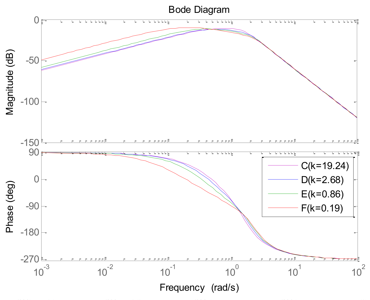
Figure 8.
The time response of process for points A, B, C, and G. Load disturbance is introduced at t = 25 s.
Figure 8.
The time response of process for points A, B, C, and G. Load disturbance is introduced at t = 25 s.

Figure 9.
The closed-loop setpoint frequency response of the process for points A, B, C, and G.

Figure 10.
The closed-loop load disturbance frequency response of the process for points A, B, C, and G.
Figure 10.
The closed-loop load disturbance frequency response of the process for points A, B, C, and G.

Figure 11.
The contours.
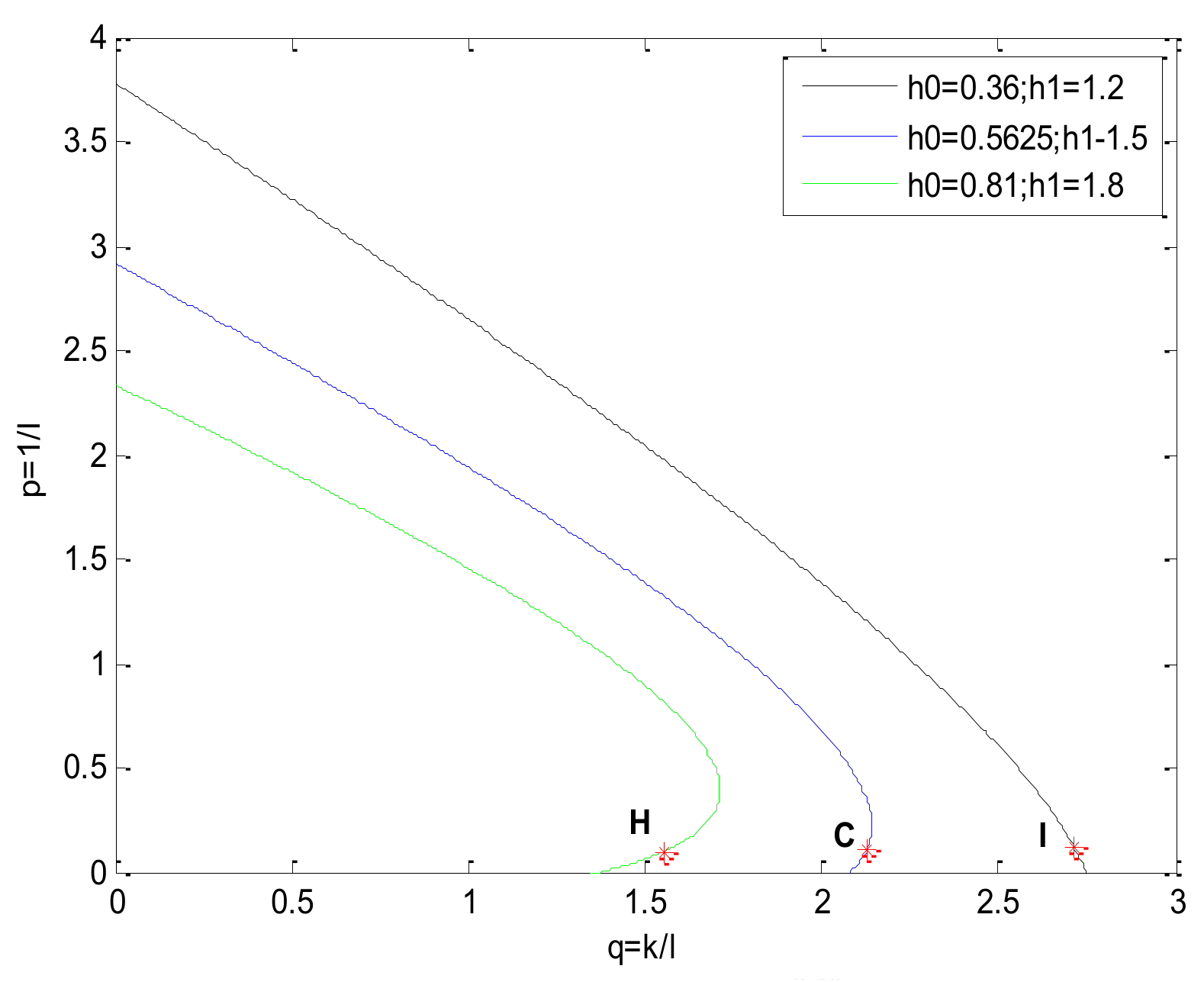
Figure 12.
The closed-loop time response of process for points H, C, and I.

Figure 13.
The closed-loop setpoint frequency response of the process for points H, C, and I.


Table 1.
The coordinates of points from A–G in the plane.
| A | B | C | D | E | F | G | |
|---|---|---|---|---|---|---|---|
| q | 1.398 | 1.689 | 2.128 | 1.967 | 1.342 | 0.4648 | 2.84 |
| p | 0.0895 | 0.0903 | 0.1106 | 0.7344 | 1.567 | 2.475 | 0.1279 |
Table 2.
The coordinate of points H, C, and I in the plane.
| H | C | I | |
|---|---|---|---|
| q | 1.546 | 2.128 | 2.712 |
| p | 0.0927 | 0.1106 | 0.1251 |
Table 3.
The closed-loop poles and the corresponding smallest m of all points A~I.
| The Closed-Loop Poles | The Smallest | ||||
|---|---|---|---|---|---|
| A | −0.868 + 1.085i | −0.868 − 0.085i | −0.632 + 0.089i | −0.632 − 0.089i | 0.8 |
| B | −0.8456 + 1.2079i | −0.8456 − 1.2079i | −0.6544 + 0.0939i | −0.6544 − 0.0939i | 0.7 |
| C | −0.8316 + 1.3859i | −0.8316 − 1.3859i | −0.6684 + 0.1071i | −0.6684 − 0.1071i | 0.6 |
| D | −0.9996 + 1.666i | −0.9996 − 1.666i | −0.5004 + 0.2067i | −0.5004 − 0.2067i | 0.6 |
| E | −1.1377 + 1.896i | −1.1377 − 1.896i | −0.3623 + 0.152i | −0.3623 − 0.152i | 0.6 |
| F | −1.2462 + 2.0772i | −1.2462 − 2.0772i | −0.3947 | −0.1129 | 0.6 |
| G | −0.8145 + 1.6289i | −0.8145 − 1.6289i | −0.6855 + 0.1083i | −0.6855 − 0.1083i | 0.5 |
| H | −0.6852 + 1.142i | −0.6852 − 1.142i | −0.8148 + 0.2052i | −0.8148 − 0.2052i | 0.6 |
| I | −0.9654 + 1.6088i | −0.9654 − 1.6088i | −0.6266 | −0.4426 | 0.6 |
Table 4.
The related parameters of the DDE−GFM and Panagopoulos’ method.
| DDE–GFM | Panagopoulos’ Method | |||||||||||
|---|---|---|---|---|---|---|---|---|---|---|---|---|
| 0.0625 | 0.5 | 0.35 | 0.6999 | 0.0863 | 1.4594 | 0.69 | 0.68 | 4.5 | 2.27 | 0 | 0.08 | |
| 0.25 | 1 | 0.5 | 0.5495 | 0.1365 | 0.5608 | 0.5458 | 0.555 | 3.21 | 1.74 | 0 | 1.61 | |
| 16 | 8 | 0.35 | 44.767 | 88.768 | 5.7393 | 44.384 | 43.13 | 0.189 | 0.13 | 0 | 0.81 | |
| 0.49 | 1.4 | 0.35 | 2.1591 | 0.7389 | 1.6449 | 2.1112 | 2.27 | 1.91 | 0.98 | 0 | 0.53 | |
| 0.25 | 1 | 0.3 | 1.6934 | 0.4118 | 1.8324 | 1.647 | 1.47 | 2.33 | 1.25 | 0 | 0.72 | |
| 0.16 | 0.8 | 0.3 | 1.3189 | 0.2605 | 1.7107 | 1.3024 | 1.15 | 2.74 | 1.49 | 0 | 0.97 | |
| 0.2025 | 0.9 | 0.4 | 0.9721 | 0.2149 | 1.1373 | 0.9549 | 0.982 | 3.14 | 1.73 | 0 | 1.24 | |
| 0.64 | 1.6 | 0.85 | 0.5757 | 0.2276 | 0.3722 | 0.5691 | 0.542 | 2.07 | 0.79 | 0 | 1.03 | |
Table 5.
The simulation results covering the position of the work point in the plane and the control signal and time response comparing the DDE−GFM and Panagopoulos’ method.
Table 5.
The simulation results covering the position of the work point in the plane and the control signal and time response comparing the DDE−GFM and Panagopoulos’ method.
| Process | Work Point in Plane | Control Signal of DDE−GFM and Panagopoulos’ Method | Time Response of DDE−GFM and Panagopoulos’ Method |
|---|---|---|---|
 |  |  | |
 |  |  | |
 |  |  | |
 |  |  | |
 |  |  | |
 |  |  | |
 |  |  | |
 |  |  |
Table 6.
The performance for the DDE−GFM and Panagopoulos’ method.
| Methods | Settling Time (s) | Overshooting (%) | IAE | ||
|---|---|---|---|---|---|
| DDE−GFM | 16.952 | 1.56 | 11.96 | 2 | |
| Panagopoulos’ | 28.678 | 16.77 | 9.252 | 2 | |
| DDE−GFM | 24.232 | 6.89 | 8.6902 | 2 | |
| Panagopoulos’ | 39.392 | 21.68 | 9.1035 | 2 | |
| DDE−GFM | 1.4 | 0 | 0.0113 | 2 | |
| Panagopoulos’ | 3.344 | 0 | 0.0058 | 2 | |
| DDE−GFM | 11.368 | 0.57 | 1.441 | 2 | |
| Panagopoulos’ | 13.022 | 23.47 | 1.3511 | 2 | |
| DDE−GFM | 15.468 | 0 | 2.4522 | 2 | |
| Panagopoulos’ | 19.429 | 27.24 | 2.749 | 2 | |
| DDE−GFM | 20.829 | 0 | 3.8433 | 2 | |
| Panagopoulos’ | 25.273 | 27.39 | 4.1654 | 2 | |
| DDE−GFM | 24.521 | 2.81 | 5.2316 | 2 | |
| Panagopoulos’ | 30.931 | 26.72 | 5.5291 | 2 | |
| DDE−GFM | 11.003 | 0 | 5.67 | 2 | |
| Panagopoulos’ | 17.027 | 10.19 | 6.1111 | 2 |
© 2018 by the authors. Licensee MDPI, Basel, Switzerland. This article is an open access article distributed under the terms and conditions of the Creative Commons Attribution (CC BY) license (http://creativecommons.org/licenses/by/4.0/).
Share and Cite
MDPI and ACS Style
Wang, X.; Yan, X.; Li, D.; Sun, L. An Approach for Setting Parameters for Two-Degree-of-Freedom PID Controllers. Algorithms 2018, 11, 48. https://doi.org/10.3390/a11040048
AMA Style
Wang X, Yan X, Li D, Sun L. An Approach for Setting Parameters for Two-Degree-of-Freedom PID Controllers. Algorithms. 2018; 11(4):48. https://doi.org/10.3390/a11040048
Chicago/Turabian StyleWang, Xinxin, Xiaoqiang Yan, Donghai Li, and Li Sun. 2018. "An Approach for Setting Parameters for Two-Degree-of-Freedom PID Controllers" Algorithms 11, no. 4: 48. https://doi.org/10.3390/a11040048
Note that from the first issue of 2016, this journal uses article numbers instead of page numbers. See further details here.