A Multi-Stage Algorithm for a Capacitated Vehicle Routing Problem with Time Constraints

Abstract

The Vehicle Routing Problem (VRP) is one of the most optimized tasks studied and it is implemented in a huge variety of industrial applications. The objective is to design a set of minimum cost paths for each vehicle in order to serve a given set of customers. Our attention is focused on a variant of VRP, the capacitated vehicle routing problem when applied to natural gas distribution networks. Managing natural gas distribution networks includes facing a variety of decisions ranging from human resources and material resources to facilities, infrastructures, and carriers. Despite the numerous papers available on vehicle routing problem, there are only a few that study and analyze the problems occurring in capillary distribution operations such as those found in a metropolitan area. Therefore, this work introduces a new algorithm based on the Saving Algorithm heuristic approach which aims to solve a Capacitated Vehicle Routing Problem with time and distance constraints. This joint algorithm minimizes the transportation costs and maximizes the workload according to customer demand within the constraints of a time window. Results from a real case study in a natural gas distribution network demonstrates the effectiveness of the approach.

1. Introduction

In the current competitive environment, manufacturing and service companies are facing different challenges: global markets, increased competition, customers behavior, accelerated lead and delivery times as well as process technology capabilities, which are contributing to an increase in uncertainty and variability [1,2]. Therefore, choosing the shortest path is mandatory to minimize costs and time and allow companies to focus on significant sustainability issues, which have become a core strategic imperative pushing companies towards identifying new opportunities [3].

The Vehicle Routing Problem (VRP) is one of the most optimized tasks studied and it is implemented in a huge variety of industrial applications. The VRP is defined as the optimal delivery route from one or multi depots to customers, taking into account distance, capacity and time constrains. VRP is used when a series of routes must be identified to optimize the distribution of goods to various cities using the most economical method with each vehicle leaving and returning from the central depot (or from several depots). The objective is to design a set of minimum cost paths for each vehicle in order to serve a given set of customers [4].

The VRP manages the design and optimization of vehicle fleets’ routes and is applied to distribution, logistics and supply chain issues. The VRP presents several variants on mathematical modelling such as capacitated VRP, multi-depot VRP, periodic VRP, split delivery VRP, stochastic VRP, VRP with backhauls, VRP with pick-up and delivery and VRP with time windows. Additionally, under a dynamic competition environment, many companies are concerned to increase logistics capabilities, especially due to the costs of allocating clients to routes and the distribution expenses included then in the total cost and adopt VRP for Product-Service-Systems (PSS) [5].

Furthermore, in the recent literature about VRP, a new trend has been gaining attention concerning the area of Internet of Things (IoT). The IoT can optimize delivery routes due to the implementation of sensors. Devices have a better connection to the internet and therefore, they can be managed at any time or place [6]. Specifically, Tsiropoulou [7,8] analyze the paradigm of machine to machine driven IoT, which aims to provide contextual services and a more energy efficient resource management approach. This provides the opportunity to adopt connecting devices, which improve the flexibility of the control and decision-making processes and enable “a mobile node’s self-optimization and self-adaptation function” [6].

Our attention is focused on the aforementioned grouping problems when applied to natural gas distribution networks (NGDNs), which deliver an energy source growing in popularity due to its low environmental impact compared to oil and coal. For these reasons, planning and optimization of NGDNs factors are critical and they are of great interest in this field of research, especially concerning metropolitan areas.

With this in mind, optimization methods and operation research techniques could reduce network logistic outlays as well as design, flow, operation and expansion costs.

Managing NGDNs includes making a variety of decisions ranging from human resources and material resources to facilities, infrastructures, and carriers.

Common problems that affect NGDNs are:

• Designing of new NGDN or expansion of existing ones [9];
• Routing a fleet of vehicles from a depot to service a set of customers that are geographically dispersed [10];
• Determining the pipelines in the network, the compressor stations and their capacities [11];
• Minimizing the transportation costs and maximizing the transported volume [12];
• Optimizing gas network inventories in the face of system uncertainties [13];
• Synchronizing the minimum risk loss and total cost of natural gas pipeline networks [14].

Despite the numerous papers available on VRP, only a few study and analyze the problems occurring in capillary distribution operations such as those found in a metropolitan area. However, there are some exceptions such as [15], where a set of field service operations are considered in order to manage the assets of a NGDN and maintain high levels of customer satisfaction and gas provider profitability, particularly regarding activation, deactivation and management of utility meters with respect to time, distance and capacity, and where an operational VRP characterized by the presence of both mandatory and not mandatory customers, and partially overlapping time windows were presented. The authors adopted a VRP with time windows (VRP-TW) combined with Simulated Annealing (SA), which allows for real constraints optimization in reasonable computational time and represents an alternative approach with respect to existing contributions to the considered subject. This algorithm interface operates as a decision support system tool that allows decision makers to both visualize and to modify the routes while allowing interesting optimization capabilities.

The implementation of the established algorithm to a real case study resulted in a far more complex system, where both running time and usability were not effective, resulting in a pilot approach which did not allow the company to adapt the changes needed or take into consideration the additional paths and real time constraints.

Accordingly, this research proposes a different algorithm which takes into account these drawbacks and suggests a new solution, that is, simplifying the problem by reducing the number of constraints and varying some variables. Hence, a true comparison of the two studies is not possible.

This work introduces a new algorithm based on the Saving Algorithm (SA) heuristic approach which aims to solve a Capacitated Vehicle Routing Problem (CVRP) with time and distance constraints. This joint algorithm minimizes the transportation costs and maximizes the workload according to customer demand within the constraints of a time window and it allows for increased effectiveness in real-time scenarios.

The paper is organized as follows: in Section 2, the problem is described. Section 3 formally presents the CVRP and the joined algorithms. Experimentation and results are shown in Section 4 and finally, in Section 5 some conclusions are drawn.

2. Problem Definition

This problem derives from a real case study concerning a small medium service enterprise, which manages domestic gas utilities in the metropolitan area of Genoa (Italy). The problem it faces is quite complex and is related to its field service operations of utility networks in the metropolitan area. The heuristic approach proposed in this paper is based on the CVRP with time constraints, and it exploits the well-known cluster-first-route-second problem decomposition technique to minimize the distance within the cluster by generalized assignment problem.

The study deals with the planning of service visits to a set of customers, performed by a set of company operators, each using a vehicle from the company fleet.

The service company provides two types of operations: Activation and Deactivation. Activation is when a new customer opens an account and deactivation is when a customer closes an account. Activations and deactivations are fixed for a specific day by the gas company provider who arranges an appointment with the customers within a specific time window.

The fleet is a set of vehicles each associated with a single driver whose workload should not exceed two-time based restrictions:

• A maximum daily workload (visits per day);
• A maximum workload for the time window (time allotted per visit).

Hence, the problem consists of finding a method to optimize company logistic resources, while maintaining a maximum level of customer satisfaction in the most economical way.

This algorithm improves the distribution efficiency and increases customer service quality using the aforementioned heuristics, the Saving Algorithm and 2-Opt.

The algorithm assigns a sequence of interventions to the various operators, which are carried out during the working day (divided into time slots) therefore minimizing the total distance traveled in compliance with the following operational constraints:

• Activation: time necessary for the operation;
• Deactivation: time necessary for the operation;
• Each operation (activation and deactivation) has an account number ID;
• Location expressed in terms of GIS coordinates (latitude and longitude);
• Time Window (TW) of the operation (

  Table 1. Time windows considered.

  Preset Daily Time Windows (TW)
  TW1	8:00–10:00
  TW2	9:00–11:00
  TW3	10:00–12:00
  TW4	13:00–15:00
  TW5	14:00–16:00
  TW6	15:00–17:00

  );
• Total time of all operations (activation and deactivation).

The algorithm calculates the distances between the various interventions and provides a solution in terms of:

• A list of interventions for each operator consisting of an account number ID, location and time window for each customer is assigned;
• The total time of each intervention (including transport time).

3. Proposed Algorithm and Formulation

The CVRP is one of the most examined VRP applications. In CVRP, the objective is to minimize the costs of the routes (similar to the generic VRP) but at the same time not exceed the load capacity of the vehicle assigned to those paths [16].

In CVRP, customer demands, locations and depots are predetermined. The depots store all the products or services ordered by customers and each vehicle leaves and returns to the same depot. Therefore, a solution is feasible if it satisfies these aspects. Note that a route must be assigned to only one vehicle.

3.1. Basic Components of CVRP

Let us give a complete graph G = (I, J, K), the notation used and the mathematical model are as follows:

Sets:
I	set of all depots
J	set of customers
K	set of vehicles
Indices:
i	depot index
j	customer index
k	route index
Parameters:
N	number of vehicles
Cij	distance between point i and j, $i, j\in I \cup J$
dj	demand operation of customer j (in terms of time)
Qk	time limit for operator k
Lj	service time at customer j
Decision variables:
$x_{ijk}$	$=\{\begin{array}{c}1, if i preceeds j on route k\\ 0, otherwise\end{array}$
$z_{ijk}$	$=\{\begin{array}{c}1, if customer j is matched to a depot i\\ 0, otherwise\end{array}$
$y_j$	$=\mathrm{cumulative}\mathrm{travel}\mathrm{and}\mathrm{service}\mathrm{time}\mathrm{up}\mathrm{through}\mathrm{customer}j,j\in J$
$U_{lk}$	$=\mathrm{auxiliary}\mathrm{variable}\mathrm{for}\mathrm{sub}-\mathrm{tour}\mathrm{elimination}\mathrm{constrains}\mathrm{in}\mathrm{route} k$

The objective function is to minimize the total distance of all vehicles given by:

$$min{\displaystyle \sum }_{iϵI\cup J}{\displaystyle \sum }_{jϵI\cup J}{\displaystyle \sum }_{kϵK}{C}_{ij}{x}_{ijk}$$

(1)

A single route has to be given to each customer:

$${\displaystyle \sum }_{kϵK}{\displaystyle \sum }_{iϵI\cup J}{x}_{ijk}=1, jϵJ$$

(2)

Each vehicle has a time capacity constraint:

$$y_j+{\displaystyle \sum }_{jϵJ}^{}{d}_j{\displaystyle \sum }_{iϵI\cup J}^{}{x}_{ijk}\le Q_k, kϵK$$

(3)

The following equation defines the sub-tour elimination constraint:

$$U_{lk}-U_{jk}+N{x}_{ijk}\le N-1, i ϵ I, l,j ϵ J, k ϵ K$$

(4)

While Equation (5) expresses the flow conservation:

$${\displaystyle \sum }_{jϵI\cup J}{x}_{ijk}-{\displaystyle \sum }_{jϵI\cup J}{x}_{jik}=0, k ϵ K, i ϵ I\cup J$$

(5)

Each route is covered by one vehicle:

$${\displaystyle \sum }_{iϵI}{\displaystyle \sum }_{jϵJ}{x}_{ijk}\le 1, k ϵ K$$

(6)

A customer is assigned to a depot only if there is a route from the aforementioned depot going to that customer:

$$-z_{ij}+{\displaystyle \sum }_{uϵI\cup J}\left(x_{iuk}+x_{uik}\right)\le 1, i ϵ I, j ϵ J, k ϵK$$

(7)

Equations (8) and (9) give the binary requirements on the decision variable:

$$x_{ijk} ϵ \left\{0,1\right\}, i ϵ I, j ϵJ, k ϵ K$$

(8)

$$z_{ik} ϵ \left\{0,1\right\}, i ϵ I, j ϵ J$$

(9)

Finally, Equation (10) defines the positive values of the auxiliary variable:

$$U_{lk}\ge 0, l ϵ J, k ϵ K$$

(10)

To summarize, the objective function (1) minimizes the total distance of all vehicles with respect to some constraints: (i) each customer is satisfied with only one route (2); (ii) the total daily time capacity of each operator (3); (iii) the sub-tour avoidance (4); (iv) the flow limits (5) and (v) route to be served (6).

CVRP is NP-hard, therefore an efficient algorithm for solving the problem to optimality is generally unavailable with respect to real scenarios. To deal with the problem efficiently and effectively, a heuristic approach such as the Saving Algorithm and 2-Opt is applied.

3.2. Proposed Algorithm

The proposed algorithm starts from the classic problem of CVRP with a time window constraint to define routes which minimize the costs and maximize the number of activations or deactivations per worker with respect to (i) a maximum daily workload and (ii) a maximum workload for each time window. Specifically, the NGDN considered in this paper provides a service, therefore there is no load capacity for the vehicles, but there is a time constraint for the number of operations per worker.

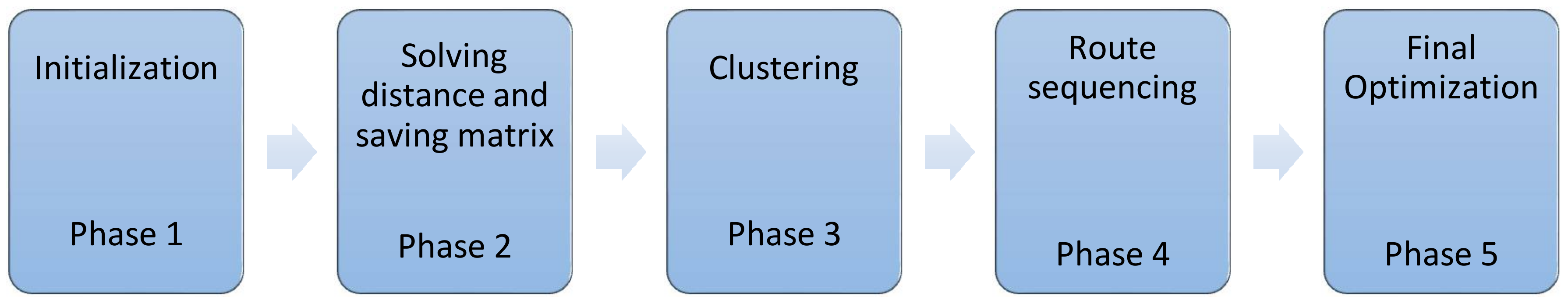
The proposed algorithm includes five phases, shown in Figure 1, that are detailed in the following.

3.2.1. Phase 1: Initialization

The first step of the algorithm is based on the initialization phase, in which all data on operation requests are collected and organized with respect to:

• Account number ID of the operation;
• Type of operation

  ◦

  Activation

  ◦

  Deactivation

• Location of the operation in terms of latitude and longitude;
• Time window for the requested intervention.

3.2.2. Phase 2: Solving Distance and Saving Matrix

The second phase of the algorithm is based on the Saving Matrix calculation, in which the distances between the depot and the customer locations are defined. At this point, it is important to underline that the case considered is based on a single depot, but equations could be extended to multi-depot problems. The Saving Matrix is calculated using the Saving Algorithm heuristic. The Saving Algorithm is a well-known heuristic for solving CVRP [17]. In the Saving Algorithm, distance and travel time savings are calculated when two routes merge together. Based on the saving order, routes are merged together sequentially and a better, more feasible solution will be generated [18].

As Figure 2 shows, the basic idea of this algorithm is to combine routes together based on the saving matrix.

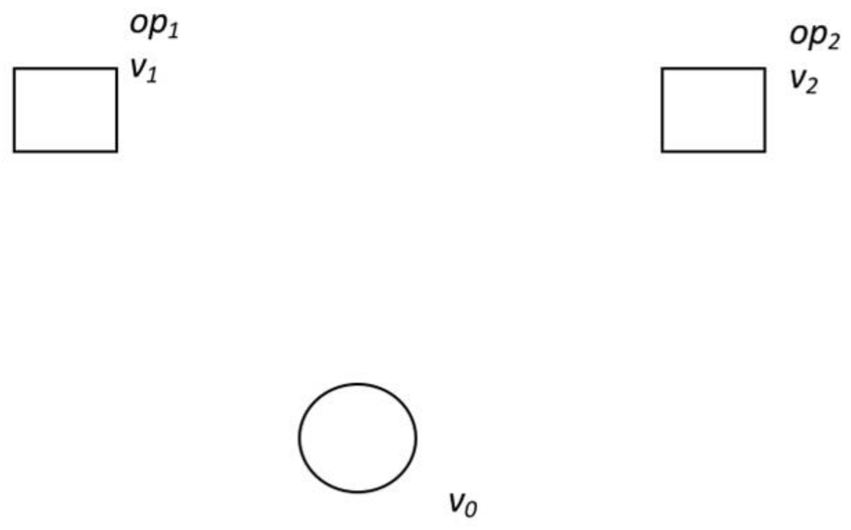
Let us give a complete graph G = (V, E), where E is the set of routes and V = {v₀, v₁, …, v_n} the set of nodes, specifically (Figure 3):

• v₀ is the depot
• v₁ and v₂ are nodes
• op_n are performed service operations

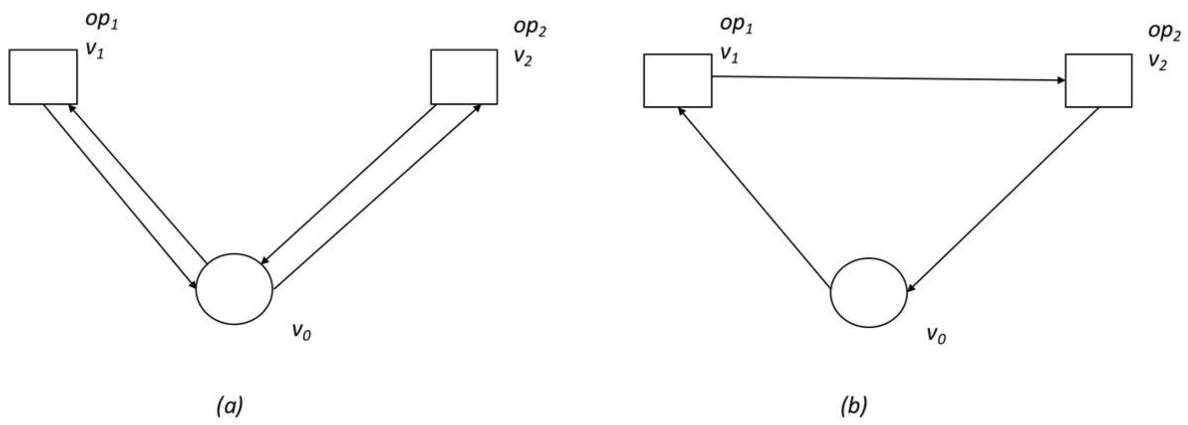
In the initial step, all nodes are connected to the depot (v₀) and N routes are generated as an initial solution (Phase 2.1). As shown in Figure 4, two different routes and policies can be generated and calculated through the Haversine formulation. It determines the great-circle distance between two points on a sphere given their longitudes and latitudes:

• Policy a: the vehicle starts from the depot, carries out the operation in v₁ and then returns to the depot, heads to v₂, carries out the operation and returns to the depot. The cost of this route is:

  $$C_a=2\overline{v_0{v}_1}+2\overline{v_0{v}_2}$$

  (11)
• Policy b: the vehicle starts from the depot, carries out the operation in v₁ and heads on to v₂, carries out the operation and returns to the depot. The cost of this route is:

  $$C_b=\overline{v_0{v}_1}+\overline{v_1{v}_2}+\overline{v_2{v}_0}$$

  (12)
  Policy b allows a saving of:

  $$S_b= C_a-C_b= 2\overline{v_0{v}_1}+2\overline{v_0{v}_2}- \overline{v_0{v}_1}-\overline{v_1{v}_2}-\overline{v_2{v}_0}$$

  (13)
  We further assume that:

  $$\overline{v_0{v}_2} = \overline{v_2{v}_0}$$

  (14)

  $$S_b= C_a-C_b= \overline{v_0{v}_1}+\overline{v_0{v}_2}-\overline{v_1{v}_2}$$

  (15)

Therefore, we can calculate the distances between all nodes of V and the savings related to them (Phase 2.2). The saving matrix is generated by calculating the saving distance and therefore the travel time for merging any two possible routes (i, j) together.

3.2.3. Phase 3: Clustering

In the clustering phase, each route is generated by grouping operations which allow maximizing the saving considering the time constraint. Based on the saving matrix, a list L(i, j) is created and sorted in descending order by merging savings. With list L(i, j), road i and road j are selected to be tested with the feasibility of mergence. If the mergence is feasible, these two roads are merged together and a new merged route is created and the saving matrix is updated with new routes. If no feasible mergence is found or it exceeds the given calculation time, the process is terminated.

In the example described above (Figure 4), we need to consider:

◦

Time window of operation performed in v₁ and v₂ = TW₁

◦

k is an operator

◦

AT_k is the available time of the worker k expressed in (min)

Policy a:

◦

Time necessary to go from node v₀ to v₁ (T₀₁) and vice versa expressed in (min)

◦

Time necessary to go from node v₀ to v₂ (T₀₂) and vice versa expressed in (min)

or Policy b:

◦

Time necessary to go from node v₁ and v₂ (T₁₂) expressed in (min)

◦

Time of the operation performed in v₁ (T₁) expressed in (min)

◦

Time of the operation performed in v₂ (T₂) expressed in (min)

Therefore, a cluster is composed of the route v₀-v₁-v₂-v₀ (Policy b) if:

$$T_{01}+T_1+T_{12}+T_2+T_{02}\le A{T}_k$$

(16)

$$T_{01}+T_1 ϵ T{W}_1$$

(17)

$$T_{12}+T_2 ϵ T{W}_1$$

(18)

Otherwise, if the time constrain expressed by Equation (16) is not verified, two routes are created and assigned to different operators (Policy a):

• v₀-v₁-v₀
• v₀-v₂-v₀

The output of this phase is the definition of the first solution, which can be improved through the next phase.

3.2.4. Phase 4: Route Sequencing

The first solution found in the second and third phase can be improved by route sequencing (maximizing savings). This means that for each route, we need to:

• Evaluate the initial solution cost, and
• Improve the current solution by a 2-Opt procedure.

This paper applies a 2-Opt local search algorithm. In each cluster, a new route will be generated by solving the 2-Opt algorithm, subdividing the original problem into sub-problems that are faced in a sequence of successive phases. In a 2-Opt algorithm, two tours are neighbors if one can be obtained from the other by deleting two edges, reversing one of the resulting two paths, and reconnecting [19]. The 2-Opt neighbors of the tour are pair-wise part exchanges within the current solution sequence [20]. For example, with n = 4 and an original solution sequence of {1, 2, 3, 4}, the six-resulting pair-wise exchanges are {2, 1, 3, 4}, {3, 2, 1, 4}, {4, 2, 3, 1}, {1, 3, 2, 4}, {1, 4, 3, 2}, and {1, 2, 4, 3}.

An exhaustive search visits all n! tours, while the total number of tours visited by 2-Opt, including the original data set, is given by the following formula:

$$\frac{n\left(n-1\right)}{2}$$

(19)

The adoption of the 2-Opt procedure allows the scalability to be optimized, as a ‘linear’ increase of computational time is expected rather than a factorial. The 2-Opt method improves the local search ability of the algorithm and its overall performance. The output of this phase is the definition of a second, improved solution.

3.2.5. Phase 5: Final Optimization

The final optimization phase aims at improving the overall solution starting from the second improved solution, attempting to maximize the available time of an operator taking into account the corresponding time window. In fact, after sequence optimization provided by the 2-Opt algorithm, there is the possibility that a route can be operated with less time than the time identified by the initial solution. Therefore, an additional operation may be added to the optimized route. Taking a look at the previous simple example (Figure 4) where:

$$T_{01}+T_1+T_{12}+T_2+T_{02}<A{T}_k$$

(20)

An additional operation can be manually introduced in order to fill AT_k. Therefore, a cluster is composed of the route v₀-v₁-v₂-v₃-v₀ (Figure 5) if:

$$T_{01}+T_1+T_{12}+T_2+T_{02}+T_{23}+T_3+T_{30}<A{T}_k$$

(21)

$$T_{23}+T_3 ϵ T{W}_1$$

(22)

where:

• Time necessary to go from node v₂ and v₃ (T₂₃) expressed in (min)
• Time of the operation performed in v₃ (T₃) expressed in (min)

4. A Real-Case Scenario Application of the Proposed Algorithm

In this section, a real-case scenario application of the proposed algorithm is provided. The problem is composed of 54 activations and 51 deactivations (for a total of 105 service operations) which need to be assigned to workers; each operation is described with an account number ID, the location and the time in which the operation has to be completed, an example of the sample is reported in

Table 2. Sample of output dataset expressed in GIS coordinates and relative TW.

ID	Type of Operation	Latitude	Longitude	ID TW
0	Depot	44.100546	8.9401007
5	Activation	44.4039594	8.9372752	TW1
52	Activation	44.4052182	8.9393867	TW6
29	Activation	44.4025486	8.9376078	TW5
57	Deactivation	44.4046075	8.9328502	TW1
78	Deactivation	44.4104947	8.9323900	TW6

.

The algorithm was implemented on a Windows 10 × 64, Intel Core i7 CPU 2.40 GHZ, 4 GB RAM.

After all the data from the activations and deactivations have been collected (Phase 1), the algorithm provides a solution taking into account all constraints and then allocates operations to the workers, solving the aforementioned Phases 2, 3, 4 as shown in

Table 3. Solution₍₄₎ provided by the proposed algorithm for TW1.

TW1	Number of Requested Operators	Number of Operations	Activations	Deactivations
8:00–10:00	9	22	11	11
120 min
	Operations ID				Allocated Time (min)	Not Allocated Time (min)
Operator 1	70	17	72		77.2	42.8
Operator 2	66	63	65	71	77.4	42.6
Operator 3	20	19			81.0	39.0
Operator 4	64	13	56		68.9	51.1
Operator 5	57	55	5		67.5	52.5
Operator 6	2	1			65.7	54.3
Operator 7	4	3			66.3	53.7
Operator 8	62	18			49.1	70.9
Operator 9	12				56.9	63.1

.

The solution is calculated thanks to the definition of distance and saving matrix for each pair of destinations. Table 3 shows the account number IDs assigned to an operator in time window 1. The two last columns represent the total time of intervention (including transport time) and the not allocated time for each operator, respectively.

Table 3 shows that the operator 1 carries out the interventions for IDs 70, 17 and 72 with a total intervention time of 77.2 min, consisting of 60 min of operating time (2 deactivations and 1 activation) and 17 min of travel time.

Then,

Table 4. Workload assigned to each operator.

	Total TW1 (min)	Total TW2 (min)	Total TW3 (min)	Total TW4 (min)	Total TW5 (min)	Total TW6 (min)	Total Workload per Operator per Day (min)
Operator 1	76.00	56.71	0.00	53.00	33.00	55.10	274.30
Operator 2	74.40	47.24	0.00	58.00	49.00	32.85	261.80
Operator 3	73.80	48.99	20.00	47.00	32.00	49.95	272.00
Operator 4	68.90	47.46	47.00	58.00	0.00	65.57	286.50
Operator 5	66.00	32.29	49.00	54.00	44.00	0.00	245.20
Operator 6	65.50	37.35	0.00	57.00	49.00	55.95	264.20
Operator 7	65.50	58.87	0.00	65.00	52.00	34.94	275.50
Operator 8	49.10	47.68	51.00	34.00	31.00	47.72	260.90
Operator 9	56.90	0.00	0.00	64.00	50.00	38.81	209.50
Operator 10	0.00	0.00	0.00	50.00	50.00	35.95	135.50
Operator 11	0.00	0.00	0.00	30.00	51.00	36.22	117.00
Operator 12	0.00	0.00	0.00	30.00	30.00	32.13	92.60
Operator 13	0.00	0.00	0.00	15.00	42.00	57.89	114.50

reports the workload that has been assigned to each operator throughout the day and information related to the operating time (including travel time) for the whole day.

Finally, in order to optimize routes (Phase 5),

Table 5. Example of support for route optimization (Phase 5).

Operators	IDs				Operators	IDs				Operators	IDs
Operator 1	70	17	72		Operator 1	70	17	72		Operator 1	70	17	72
Operator 2	66	63	65	71	Operator 2	66	63	65	71	Operator 2	66	63	65	71
Operator 3	20	19			Operator 3	20	19			Operator 3	20	19
Operator 4	64	13	56		Operator 4	64	13	56		Operator 4	64	13	56
Operator 5	57	55	5		Operator 5	57	55	5		Operator 5	57	55	5
Operator 6	2	1			Operator 6	2	1			Operator 6	2	1
Operator 7	4	3			Operator 7	4	3			Operator 7	4	3
Operator 8	62	18			Operator 8	62	18			Operator 8	62	18	12
Operator 9	12				Operator 9	12
Before Phase 5					Distance from intervention 12 to all those located in the TW1					After Phase 5

Green: distance less than 3 km; Yellow: distance between 3 and 6 km; Red: distance greater than 6 km.

shows the distance from one location to all those located in the same time window. According to Table 5 the position of intervention ID 12 would be close to interventions ID 2, 1, 4, 3, 62 and ID 18, quite close to interventions ID 70, 17, 72, 64, 13, 56, 57, 55, and ID 5 and distant from the remaining ones. Through this color scale the user can see at a simple glance any useful movements and make the appropriate changes in order to optimize the routes once again. In the example presented here, the intervention ID 12 is moved from operator 9 to operator 8 respecting the AT₈. Indeed, AT₈ before the Phase 5 was 49.1 min, by adding intervention ID 12, it totals106 min, which is less than the maximum available time established at 120 min.

Table 6. Dispatching list assigned to operator 8.

ID	Time Window
62	TW1
18	TW1
12	TW1
67	TW2
6	TW2
61	TW3
10	TW3
25	TW4
29	TW5
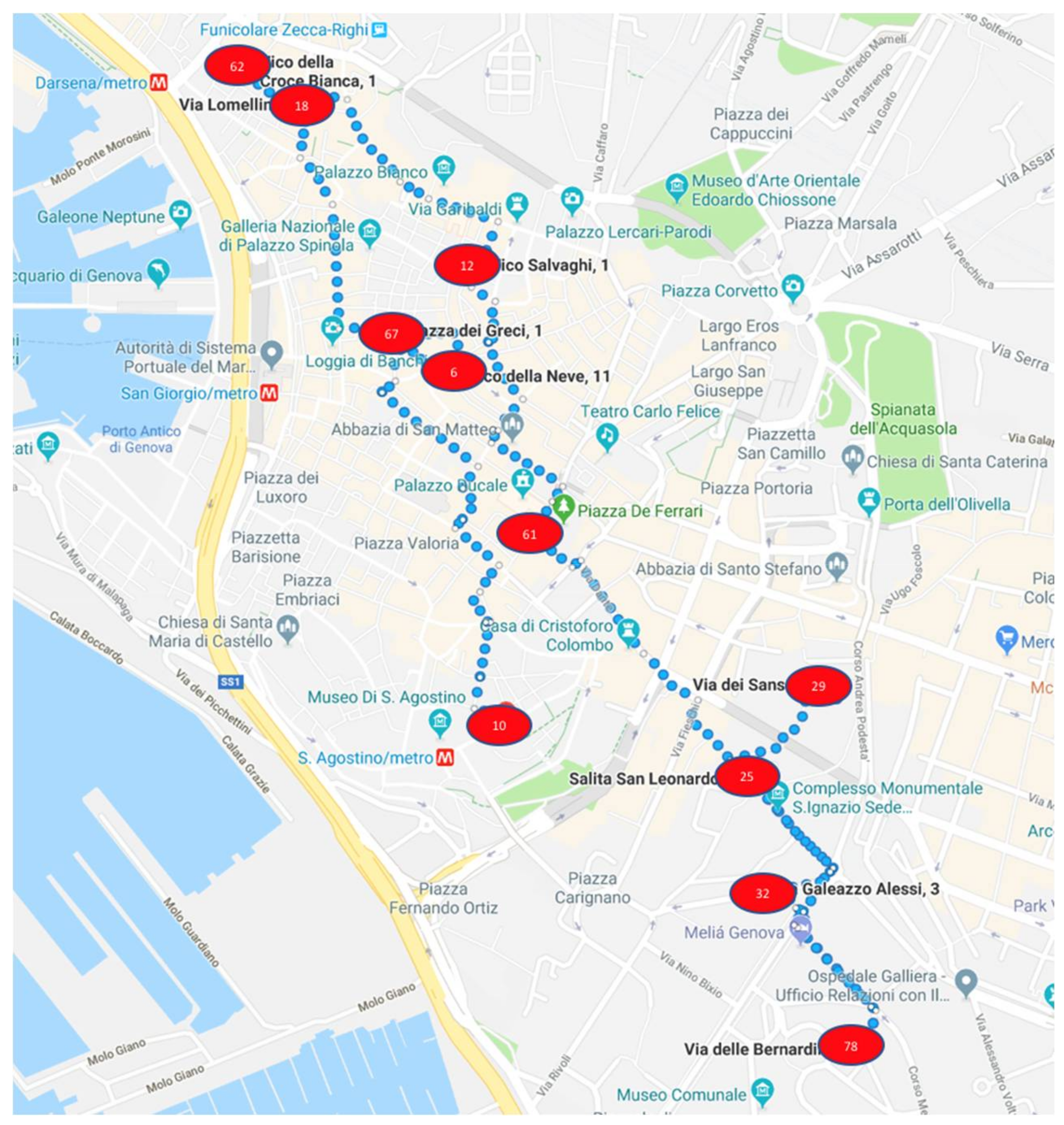
32	TW6
78	TW6

and Figure 6 show the information relating to the itineraries defined after Phase 5 for Operator 8. It contains information on each intervention assigned to him, such as the type and time window in which it is located and the visual path.

Finally, a comparison between the algorithm provided by [13] and the one proposed in this paper is shown. It takes into account:

• The running time necessary for the algorithm to provide the solution;
• The imbalance;
• The total workload for a set of operators.

The comparison deals with the problem, which as previously described is composed of 54 activations and 51 deactivations (reported in Table 2).

Table 7. Comparison between the previous and the current work.

	Number of Operators	Total Daily Workload (min)	Daily Imbalance per Operator (min)	Running Time (min)
Paolucci et al. 2018	9	2673.2	182.9	12.7
Proposed algorithm	13	2809.5	263.8	3

reports the results of the comparison. In particularly, there is an interesting decrease in running time (the computation time in minutes) as the total running time of the previous algorithm is 8.5 min while the proposed algorithm is completed in 3 min. Clearly, the difference between the two running times depends on the fact that the first algorithm takes into account more constraints with respect to the second solution, such as:

• The load capacity (difficulty level of interventions) for the vehicle: the vehicle has a strict capacity, there is a maximum daily score per vehicle;
• The workload for a worker: it takes into account the maximum daily score per operator, the maximum score per time window and additionally the maximum score per type of operation.

In light of the explanation above, it is important to point out that the solution provided by the proposed algorithm is clearly unfavorable. As Table 7 shows, the previous algorithm requires 9 operators and a total workload of 2673.2 while the current algorithm proposes 13 operators with a total workload of 2809.5. Furthermore, the imbalance increases from 182.9 min per operator per day in the previous case to 263.8 min in the case of the proposed algorithm.

The analyzed operations (51 activations and 54 deactivations) represent the real data set analyzed and managed by the pilot company. In terms of time performance, by using a heuristic approach, a ‘linear’ increase in computational time would be expected in the case of a greater number of operations to be managed. Here, it is important to note that the proposed approach stems from the evident limitations of a previous math-heuristic approach that the authors developed to address the same problem. After almost a year of the pilot phase, the company showed difficulties in setting up and maintaining the set of constraints, as well as in adding or removing constraints and in managing frequent variations and unforeseen events occurring during day-by-day operations. Hence, the proposed approach is less ‘optimal’ (by using a set of heuristics) but allows the company to iteratively re-allocate operators to modified conditions in less time and in an easier way, thus, providing a more robust and effective solution to the real-time scenario. The benefits of the proposed approach are not just about pure performance but are related to its usability and applicability (less computational time, less constraints to be managed by adopting an appropriate simplification, better reactivity) and the ability to dynamically generate solution routes.

To conclude, the previous algorithm performs well but it is less effective in a real-case scenario, as the case study pilot phase demonstrated. Clearly the performance of our approach is lesser but its ability to manage the real case scenario is greatly improved, showing that more interactive and easy-to-parametrize “optimization” algorithms could be more effective depending on the application context.

5. Conclusions

The proposed algorithm based on the Saving Algorithm heuristic approach which aims to solve a Capacitated Vehicle Routing Problem (CVRP) with time and distance constraints was developed. This paper starts with the results of a practical application to a real scenario as reported by [13], where an operational VRP characterized by the presence of both mandatory and not mandatory customers and partially overlapping time windows was presented. The authors adopted a VRP with time windows (VRP-TW) combined with Simulated Annealing (SA), which allows for real constraints optimization in reasonable computational time and represents an alternative approach with respect to existing contributions.

The implementation of the previous algorithm to the real scenario resulted in an overly complex system setting to manage all constraints and both the running time and usability were not effective. Furthermore, the highly-sophisticated optimization model was difficult to modify and maintain by the company, for example, to implement new additional paths and constraints. Because of these limitations, the presented paper proposes a reasonable reduction in complexity (accepted by the service company) in order to design and implement a multi-stage algorithm to solve the reduced problem. The heuristic approach proposed in this paper, based on the CVRP with time constraints, effectively tackles the complex problem regarding the field service operations of utility networks in a metropolitan area, by exploiting the well-known “cluster-first-route-second” problem decomposition technique to minimize the distance within the cluster by generalized assignment problem. In each cluster, a new route is generated by solving the 2-Opt, subdividing the original problem into sub-problems that are faced in a sequence of successive phases. This algorithm minimizes the transportation costs and maximizes the workload according to customer demand within the constraints of time window.

Advantages, documented by the results provided from the practical application of this algorithm, are:

• The results demonstrated the efficiency of the approach in tackling a complex optimization task by providing highly pragmatic and realistic time-responsive solutions;
• Flexibility since it can be applied to different routing problems not only to NGDNs;
• Increased “adaptability” thanks to an implemented approach of optimizing routes (greater parametrization freedom), taking into account the different constraints, depending on the specific problem under study.

As a future study, this new approach can be tested and compared with some additional comparative numerical results from other relevant research works in order to show the benefit of adopting this proposed framework. Additionally, future developments could be the real-time connection of operators to this heuristic reactive approach in order to know the state and location of operators and to improve their allocation with respect to service visits inserted in the time window.

References

- Burger, N.; Demartini, M.; Tonelli, F.; Bodendorf, F.; Testa, C. Investigating flexibility as a performance dimension of a Manufacturing Value Modeling Methodology (MVMM): A framework for identifying flexibility types in manufacturing systems. Procedia CIRP 2017, 63, 33–38. [Google Scholar] [CrossRef]
- Tonelli, F.; Paolucci, M.; Anghinolfi, D.; Taticchi, P. Production planning of mixed-model assembly lines: A huristic mixed integer programming based approach. Prod. Plan. Control 2013, 24, 110–127. [Google Scholar] [CrossRef]
- Demartini, M.; Orlandi, I.; Tonelli, F.; Anguitta, D. A Manufacturing Value Modeling Methodology (MVMM): A value mapping and assessment framework for sustainable manufacturing. In International Conference on Sustainable Design and Manufacturing; Springer: Cham, Switzerland, 2017. [Google Scholar]
- Cordeau, J.-F.; Savelsbergh, M.W.P.; Vigo, D. Chapter 6 Vehicle Routing. In Handbooks in Operations Research and Management Science; Elsevier: New York, NY, USA, 2007; Volume 14, pp. 367–428. [Google Scholar]
- Tonelli, F.; Taticchi, P.; Sue, E.S. A framework for assessment and implementation of product-service systems strategies: Learning from an action research in the health-case sector. WSEAS Trans. Bus. Econ. 2009, 6, 303–319. [Google Scholar]
- Mazayev, A.; Correia, N.; Schütz, G. Data Gathering in Wireless Sensor Networks Using Unmanned Aerial Vehicles. Int. J. Wirel. Inf. Netw. 2016, 23, 297–309. [Google Scholar] [CrossRef]
- Tsiropoulou, E.E.; Mitsis, G.; Papavassiliou, S. Interest-aware energy collection & resource management in machine to machine communications. Ad Hoc Netw. 2018, 68, 48–57. [Google Scholar]
- Tsiropoulou, E.E.; Paruchuri, S.T.; Baras, J.S. Interest, energy and physical-aware coalition formation and resource allocation in smart IoT applications. In Proceedings of the 51st Annual Conference on Information Sciences and Systems (CISS), Baltimore, MD, USA, 22–24 March 2017. [Google Scholar]
- Mikolajková, M.; Haikarainen, C.; Saxén, H.; Pettersson, F. Optimization of a natural gas distribution network with potential future extensions. Energy 2017, 125, 848–859. [Google Scholar] [CrossRef]
- Sungur, I.; Ordóñez, F.; Dessouky, M.M. A robust optimization approach for the capacitated vehicle routing problem with demand uncertainty. IIE Trans. 2008, 40, 509–523. [Google Scholar] [CrossRef]
- Üster, H.; Dilaveroğlu, Ş. Optimization for design and operation of natural gas transmission networks. Appl. Energy 2014, 133, 56–69. [Google Scholar] [CrossRef]
- Alves, F.d.; de Souza, J.N.M.; Costa, A.L.H. Multi-objective design optimization of natural gas transmission networks. Comput. Chem. Eng. 2016, 93, 212–220. [Google Scholar] [CrossRef]
- Zavala, V.M. Stochastic optimal control model for natural gas networks. Comput. Chem. Eng. 2014, 64, 103–113. [Google Scholar] [CrossRef]
- An, J.; Peng, S. Layout optimization of natural gas network planning: Synchronizing minimum risk loss with total cost. J. Nat. Gas Sci. Eng. 2016, 33, 255–263. [Google Scholar] [CrossRef]
- Paolucci, M.; Anghinolfi, D.; Tonelli, F. Field services design and management of natural gas distribution networks: A class of vehicle routing problem with time windows approach. Int. J. Prod. Res. 2017, 56, 1–17. [Google Scholar] [CrossRef]
- Federgruen, A.; Simchi-Levi, D. Chapter 4 Analysis of vehicle routing and inventory-routing problems. In Handbooks in Operations Research and Management Science; Elsevier: New York, NY, USA, 1995; Volume 8, pp. 297–373. [Google Scholar]
- Caccetta, L.; Alameen, M.; Abdul-Niby, M. An Improved Clarke and Wright Algorithm to Solve the Capacitated Vehicle Routing Problem. Technol. Appl. Sci. Res. 2013, 3, 413–415. [Google Scholar]
- Pan, H.; Li, W. Hybrid Genetic-Saving Algorithm and Its Application in Vehicle Routing Problem. In Proceedings of the International Conference on Management and Service Science, Wuhan, China, 20–22 September 2009; pp. 1–4. [Google Scholar]
- Zhao, Y.; Leng, L.; Qian, Z.; Wang, W. A Discrete Hybrid Invasive Weed Optimization Algorithm for the Capacitated Vehicle Routing Problem. Procedia Comput. Sci. 2016, 91, 978–987. [Google Scholar] [CrossRef]
- Bräysy, O.; Gendreau, M. Vehicle Routing Problem with Time Windows, Part I : Route Construction and Local Search Algorithms. Transp. Sci. 2005, 39, 104–118. [Google Scholar] [CrossRef]
Figure 1.
The phases of the proposed algorithm.
Figure 2.
Flowchart of Saving Algorithm.
Figure 3.
Example of nodes.
Figure 4.
Example of routes between nodes.
Figure 5.
Improved path.
Figure 6.
Path of operator 8.