Gray Wolf Optimization Algorithm for Multi-Constraints Second-Order Stochastic Dominance Portfolio Optimization


1
College of Information Science & Technology, Hainan University, No. 58 Renmin Avenue, Haikou 570228, China
2
School of Economic and Management, Hainan University, No. 58 Renmin Avenue, Haikou 570228, China
3
State Key Laboratory of Marine Resource Utilization in the South China Sea, Hainan University, No. 58 Renmin Avenue, Haikou 570228, China
*
Author to whom correspondence should be addressed.
Algorithms 2018, 11(5), 72; https://doi.org/10.3390/a11050072
Submission received: 11 April 2018
/
Revised: 10 May 2018
/
Accepted: 11 May 2018
/
Published: 15 May 2018
(This article belongs to the Special Issue Algorithms in Computational Finance)
Abstract
:In the field of investment, how to construct a suitable portfolio based on historical data is still an important issue. The second-order stochastic dominant constraint is a branch of the stochastic dominant constraint theory. However, only considering the second-order stochastic dominant constraints does not conform to the investment environment under realistic conditions. Therefore, we added a series of constraints into basic portfolio optimization model, which reflect the realistic investment environment, such as skewness and kurtosis. In addition, we consider two kinds of risk measures: conditional value at risk and value at risk. Most important of all, in this paper, we introduce Gray Wolf Optimization (GWO) algorithm into portfolio optimization model, which simulates the gray wolf’s social hierarchy and predatory behavior. In the numerical experiments, we compare the GWO algorithm with Particle Swarm Optimization (PSO) algorithm and Genetic Algorithm (GA). The experimental results show that GWO algorithm not only shows better optimization ability and optimization efficiency, but also the portfolio optimized by GWO algorithm has a better performance than FTSE100 index, which prove that GWO algorithm has a great potential in portfolio optimization.
1. Introduction
Since the mean-variance (MV) model is proposed by Markowitz [1,2], the portfolio optimization problem has attracted a lot of attention. In MV model, variance is used as the risk measure, and it is assumed that returns are normally or elliptically distributed [3]. However, Chunhachinda et al. [4] point out that the return to the world’s fourteen major stock market is not normally distributed, which means MV model lacks effectiveness in practical applications. Besides, variance counts both upward and downward deviation, which is contrary to the definition of investment risk. Later, to supply the gap, Markowitz [5] replaces the risk measure with the semi-variance, which only counts downward deviation. In addition, Konno [6] and Speranza [7] introduce the mean absolute deviation (MAD) into portfolio optimization model as risk measure. MAD reduces the sensitivity of risk, while it is difficult to do differential operation. Generally speaking, these risk measures are rather abstract. As a new type of risk measure, value at risk (VaR) is put forward in the mid-90s. Roughly speaking, VaR is a maximum quantile of the random loss in a specified period with some confidence level [8]. However, VaR also has some limitations. For example, Artzner et al. [9] point out that VaR is not a coherent measure of risk. Therefore, as an improvement on VaR, conditional value at risk (CVaR) gets widely applications in the field of portfolio optimization.
Other than Markowitz MV model, the stochastic dominance (SD) model is another important model for solving portfolio optimization problem. SD is proposed by Fishburn [10], then, Dentcheva and Ruszczynski [11] introduce SD constraint into portfolio optimization model, which takes the risk appetite into consideration and is more suited to the investors in realistic investment environments. Thereinto, in the SD model, we mainly consider first-order stochastic dominance (FSD) constraint and second-order stochastic dominance (SSD) constraint. Besides, Leshno and Levy [12] establish almost stochastic dominance (ASD) rules which formally reveal a preference for most decision makers, but not for all of them. Moreover, Javanmardi and Lawryshyn [13] introduce a new second-order stochastic dominance efficiency model called SSD-DP model, which doesn’t require a benchmark portfolio.
On the basic of MV model and SD model, scholars refine their models by adding a series of objectives or constraints into it. Arditti [14] points out that skewness has great importances of financial economics. Then, Yu et al. [15] and Bhattacharyya et al. [16] study and develop the mean-variance-skewness (MVS) model, which introduce skewness into MV model as one of the objectives. Recently, Pouya et al. [17] add criterion and experts’ recommendations on market sectors to the primary MV model as two objectives. Moreover, Soleimani et al. [18] take sector capitalization constraint into account. Generally speaking, the optimization of MV model and SD model allows these models to be more widely used in realistic investment environments.
After adding these objectives to portfolio optimization model, the original single-objective portfolio optimization problem has become a multi-objective optimization problem. Recently, Macedo et al. [19] introduce the multi-objective evolutionary algorithms (MOEAs), including non-dominated sorting genetic algorithm II (NSGA-II) and strength pareto evolutionary algorithm II (SPEA-II), into solving mean-semivariance framework model. However, the portfolio optimization entails considering competing and conflicting objectives, it’s unlikely that a portfolio can solve the multi-objectives problem simultaneously [20]. Besides, normally multi-objective optimization problem is transformed into a single-objective programming model by using fuzzy programming approach, such as Chen et al. [21]. Therefore, in this paper, we take skewness, kurtosis, CVaR or VaR into SSD framework as constraints, which we called it MCVSK and MVSK model respectively. What’s more, we only use return as the objective.
Inspired by the level of leadership and hunting mechanisms of the Grey Wolf, Mirjalili proposed Gray Wolf Optimization Algorithm, which simulates the gray wolf’s social hierarchy and predatory behavior [22]. Compared with Immune particle swarm optimization (IPSO), Ant colony algrothrim (ACA), GA, and Biogeography-based optimization(BBO), GWO has a simple structure and fast convergence. Further details about bioinspired algorithms can be found in the literature [23,24]. In the GWO algorithm, the hunting behavior is performed by and follows the first three to track the cocoon of the prey and finally complete the predation task. Recently, GWO is used to improve the classification performance of Convolutional Neural Network (CNN) models. Kumaran N et al. [25] propose a hybrid CNN-GWO approach for the recognition of human actions from the unconstrained videos, the experimental validation of this approach shows better achievable results on the recognition of human actions with recognition accuracy. Besides, Mustaffa Z et al. [26] use GWO to train Least Squares Support Vector Machine (LSSVM) for price forecasting and present a hybrid forecasting model. In this paper, GWO algorithm is used to solve MCVSK and MVSK portfolio optimization model. Besides, we compare GWO algorithm with PSO algorithm and GA in numerical experiments.
The rest of the paper is organized as follows. In Section 2, we discuss the MCVSK and MVSK portfolio optimization model respectively. In Section 3, we discuss the GWO algorithm for MCVSK and MVSK portfolio optimization model. In Section 4, we conduct numerical experiments and analyse the result of experiments. In Section 5, we summarize the performance of MCVSK and MVSK portfolio optimization model.
2. The MCVSK and MVSK Portfolio Optimization Model
2.1. The Measure of Return and Risk
As the most fundamental objective, the return to the portfolio always catches investors’ attention. In the portfolio optimization problem, our aim is to invest our capital in some assets in order to obtain some desirable characteristics of the total return on investment.
Let n denote the number of assets, which are available for investment in the beginning of a fixed period, and we assume that we have a fixed capital to be invested in them. Then we use to denote the fractions of initial capital invested in n assets. Thereinto, , where is the capital invested in asset i and w is the total amount of capital to be invested. Let X denote a set of feasible portfolios where , and it is clear that is a bound convex polyhedron. Besides, let , denote the return of asset i in the case of discrete distribution, where is a random vector on probability space () [27]. and we assume that for all . In a word, if we have a fixed capital, the return to portfolio can then be formulated as:
The measure of risk has many forms, such as variance, semi-variance, mean absolute variance, VaR, CVaR and so on. Variance is the risk measure of Markowitz MV model, which has a long history and a wide range of applications. On the basic of variance, semi-variance, mean absolute variance and other risk measures are appeared. In this paper, we mainly study two kinds of risk measures: VaR and CVaR. VaR is one of the most well-known downside risk measures due to its intuitive meaning and wide spectra of applications in practice [8]. For a fixed level , the value at risk is defined as the -quantile of the cumulative distribution function [28]:
where . However, VaR still has several noticeable limitations and drawbacks. For example, it’s insensitive to the magnitude of losses beyond VaR, and it’s not a coherent risk measure [9]. Meanwhile, CVaR measures the conditional expectation of losses beyond VaR, which is a coherent risk measure. Therefore, CVaR is theoretically more attractive and partly resolve the shortcomings of VaR [29]. The CVaR is defined as the solution to an optimization problem:
where . Besides, for smooth , CVaR equals the conditional expectation of Y [30]:
2.2. The Second-Order Stochastic Dominance Constraint
The theory of stochastic dominance originates from the theory of discrete stochastic variable optimization, and later develops into the theory of generalized stochastic variable optimization, which is widely used in economic and financial fields nowadays. In the stochastic dominance theory, the comparison between random variables is under their k-order distribution function . Assuming that there are portfolios X and Y, and the utility function of all investors is monotonically increasing. If all the investors prefer portfolio X to portfolio Y, or believe that there are only part of them is no difference, then we say portfolio X stochastically dominates portfolio Y in the first order [31].
Let x and y be the decision vectors and be the random variable, it’s said that stochastically dominates in the first order, denoted by , if:
where is the concave continuous function both in x and , is the cumulative distribution function of . For a random variable X, the first order distribution function of X is its right-continuous cumulative distribution function:
In portfolio optimization problem, SSD is of interest because, for any decision maker with risk-averse and non-satiable preferences, a portfolio which dominates a benchmark portfolio is preferred to the benchmark [32]. Based on the definition of first-order stochastic dominance, we denote stochastically dominates in the second order by , if:
Thereinto, for two different profolios X and Y, the strict dominance relation is defined as follows:
Fábián et al. [33] and Ogryczak et al. [34] prove that SSD is equivalent to the following two inequalities:
where denotes the expected value with respect to the probability distribution of . Moreover, for any increasing and concave utility function u, the following inequality exists:
where and are two random variables, and they may represent the returns of two portfolios x and y[33]. Besides, let X and Y denote two different profolios, Noyan and Rudolf [35] point out that the SSD constraint is equivalent to the continuum of CVaR constraints for all confidence levels :
2.3. The Skewness and Kurtosis Constraints
In order to get a more practical result by portfolio optimization model, many scholars try to achieve this goal by adding several objectives and constraints into the model. For example, Soleimani et al. [18] introduce transaction cost, cardinality constraints and market capitalization into Markowitz MV model as constraints, which is optimized by genetic algorithm. Besides, Lwin et al. [3] introduce some real-world constraints, such as cardinality, quantity, pre-assignment, round-lot and class constraints, into Markowitz MV model. In this paper, we mainly consider the skewness and kurtosis constraints.
About transaction costs, Yoshimoto [36] points out that ignore the transaction costs will lead to very ineffective portfolio implementation. Briefly, transaction costs can be used to model a number of costs, such as brokerage fees, bid-ask spreads, taxes, or even fund load. Supposing the transaction cost to be a V-shaped function of the difference between a given portfolio and a new portfolio , which is incorporated into the portfolio return. Therefore, the transaction cost of asset and total transaction cost can be expressed as follows [37]:
Generally speaking, the transaction cost can be modelled as the sum of fixed and variable cost [38]. In this paper, we only consider the situation under a single period, so we assume that the transaction cost is as a relatively exogenous variable.
Chunhachinda et al. [4] point out that higher moments, including skewness and kurtosis, can’t be neglected in the portfolio selection, which has great importances of financial economics. As shown by Arditti [14], the investor’s preference for more skewness to less is consistent with the notion of decreasing absolute risk aversion, because a positive-skewness asset return refers to a right-hand elongated tail of density function of asset return. Let be an uncertain variable with finite expected value e, the skewness and kurtosis of are respectively given by Equations (14) and (15):
2.4. The MCVSK and MVSK Portfolio Optimization Model
Above all, in this paper, we mainly study the following MCVSK portfolio optimization model:
where y is benchmark investment, such as FTSE100 index portfolio. Towards the objective function , we mainly consider the following two forms [31]:
where x is the investment proportion vector and is a vector represents the return of assets. Thereinto, the Equation (17) is relatively simple and the Equation (18) is more complicated. For Equation (18) takes the impact on transaction cost into consideration, which prefer the big amounts investment in portfolio. Besides, the first three constraints on the MCVSK model represent the SSD, skewness and kurtosis constraints respectively. It is worth mentioning that we combine the CVaR with the return to portfolio, which is introduced into the MCVSK model as a new constraint. This constraint is mainly inspired by behavioral economics. We think the risk which investors can bear should not a fixed value. It is obvious that the more return of portfolio, the higher risk we should bear. Moreover, we don’t consider the short-selling, so X can be expressed as follows:
In practical application, in order to ensure the diversity of portfolio, the upper bound on the fraction of capital invested in each asset is set to a relatively low vaule, and the specific value is adjusted by the number of assets available for investment. Meanwhile, as a comparison, we change the risk measure in MCVSK model into VaR and propose the following MVSK portfolio optimization model:
3. The GWO Algorithm for the MCVSK and MVSK Portfolio Optimization Model
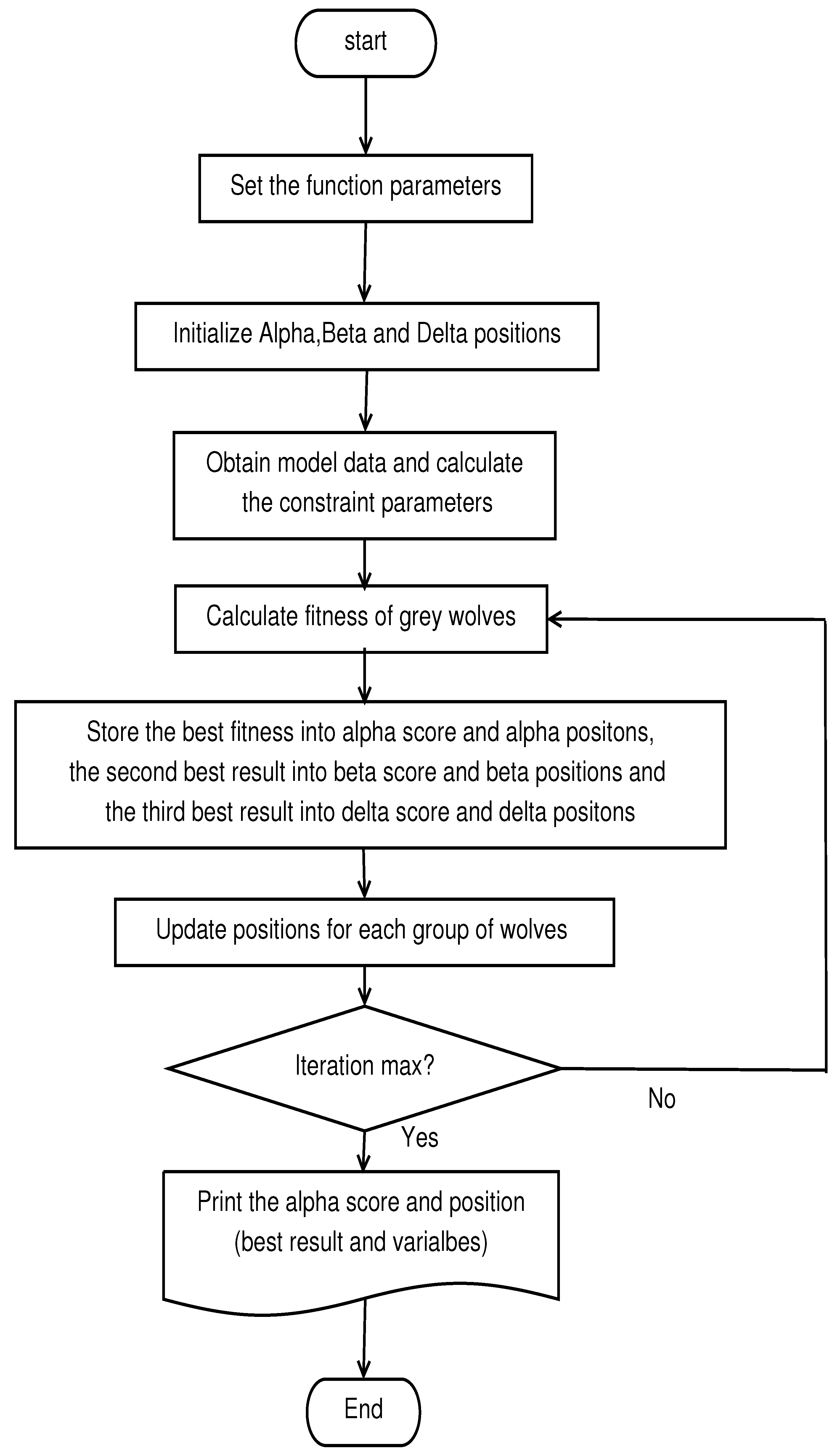
Grey Wolf Optimization algorithm is a developed metaheuristic search algorithm inspired by grey wolves proposed by Mirjalili, it be used to solve nonconvex engineering optimization problem, which simulate the social stratum and hunting mechanism of grey wolves in nature. The grey wolves being organized into four main levels [39] wolves are the leaders and their responsibility is making decisions. wolves are second-level wolves that help wolves in taking decisions or the other activities. wolf is the best candidate to be the next wolf. wolves executes and instructions but can direct other underlying individuals. Their responsibilities are scouts, sentinels, elders, hunters, and caretakers. wolves are fourth-level wolves and acts as an executor throughout the wolves. Besides, GWO are based on three main steps: searching prey, encircling prey and hunting. In this section, we will mainly discuss these three steps [22].
3.1. Prey Searching
By the arbitral (random) initialization of grey wolves in the search space paves the way for the searching operation. In order to search the prey, the grey wolf takes of the diversion from one wolf to another and the wolves are merged after the detection of prey.
3.2. Prey Encirclement
The encirclement of prey initiates after the detection of prey. The encirclement characteristics can be described mathematically as follows (21)
where is the grey wolf position, is the prey position, t is the iteration number, and given by follows (22):
and are vectors given by follows:
where is linearly decreased from 2 to 0 over the course of iterations, which is given by Equation (25). and are referred to as random vectors by the limit of .
where l is the total iteration number allowed for the optimization.
3.3. Chasing (Hunting)
After the completion of prey encirclement procedure, the grey wolves focus on the hunting of prey. Alpha wolf usually leads hunting. The beta and delta wolf also participate in hunting. However, in the abstract search space, we don’t know about the best location (prey). In order to mathematically simulate the hunting behaviour of grey wolves, we suppose that the alpha (best candidate solution), beta and delta have better knowledge about the potential location of prey. Alpha, beta and delta can be replaced by Equations (26)–(28):
And the position vector of prey with respect to alpha, beta and delta wolves can be calculated using the following mathematical formulation:
The best position can be calculated from the average of alpha, beta and delta wolves as shown in Equation (32):
For the MCVSK and MVSK models, we use the return of assets as a fitness function for the gray wolf algorithm and constrain the initialized wolf pack vector to a 101-dimensional investment proportion vector. The procedure chat of the GWO algorithm is shown in Figure 1 and the GWO approach is described in Algorithm 1.
| Algorithm 1 the main procedure of GWO algorithm for the MCVSK and MVSK model. |
| Input: problem to solve, problem; number of search agents, SearchAgents no; number of iterations, Max iteration; number of variables, dim; etc |
| Output: the best portfolio and the return of the portfolio |
|
4. Numerical Experiments
We have carried out a series of numerical tests by using GWO algorithm, PSO algorithm and GA in MATLAB2014b install of a Lenovo PC with Windows 8.1 operating system and 8 GB of RAM. In the actual investment market, there are a large number of assets for investors to choose. Therefore, in the numerical experiments, we use the stocks involved in FTSE100 index as the data source. We collect 249 daily historical returns to 101 FTSE100 index assets prior to December 2016 to construct the portfolio strategy. Specifically speaking, we use the first 200 daily historical returns to construct the portfolio strategy, and the further 49 daily historical returns to an out-of-sample test. In this section, we report and analyze the test results.
4.1. Backtesting and Out-of-Sample Test
In model (16) and model (20), we have introduced the basic MCVSK model and MVSK model respectively. In this part, we use as the benchmark and we assume that short-selling is prohibited. Besides, in order to ensure the diversity of the portfolio, the upper bound on the fraction of capital invested in each asset is set to . Above all, we propose the following MCVSK model and MVSK model:
Comparing with the FTSE100 Index, we get the test results shown in Table 1 and the specific index weight data of FTSE100 Index is shown in Table A1.
In Table 1 and the rest of the tables, “” refers to the confidence level, “ algorithm ” indicates the algorithm used to optimize the MCVSK model and MVSK model, “ skew ” and “ kurt ” refer to the skewness and kurtosis of the portfolio, “ VaR ” and “ CVaR ” are two kinds of risk measures, “” means the return of portfolio, “ max ” is the largest investment ratio in the portfolio and “ time ” indicates the average running time of algorithm. Among them, the algorithm parameters are set as follows: the initial population of GWO algorithm, PSO algorithm and GA are 100, 10 and 100 respectively. In addition, the number of iterations of the above three algorithms is 12. It is worth mentioning that because the PSO algorithm has a slow speed in optimizing the portfolio optimization model, in order to ensure that the algorithm optimization process has the same time-consuming, we set the initial population of the PSO algorithm to a lower level. What’s more, we conduct thirty repeated experiments in each case.
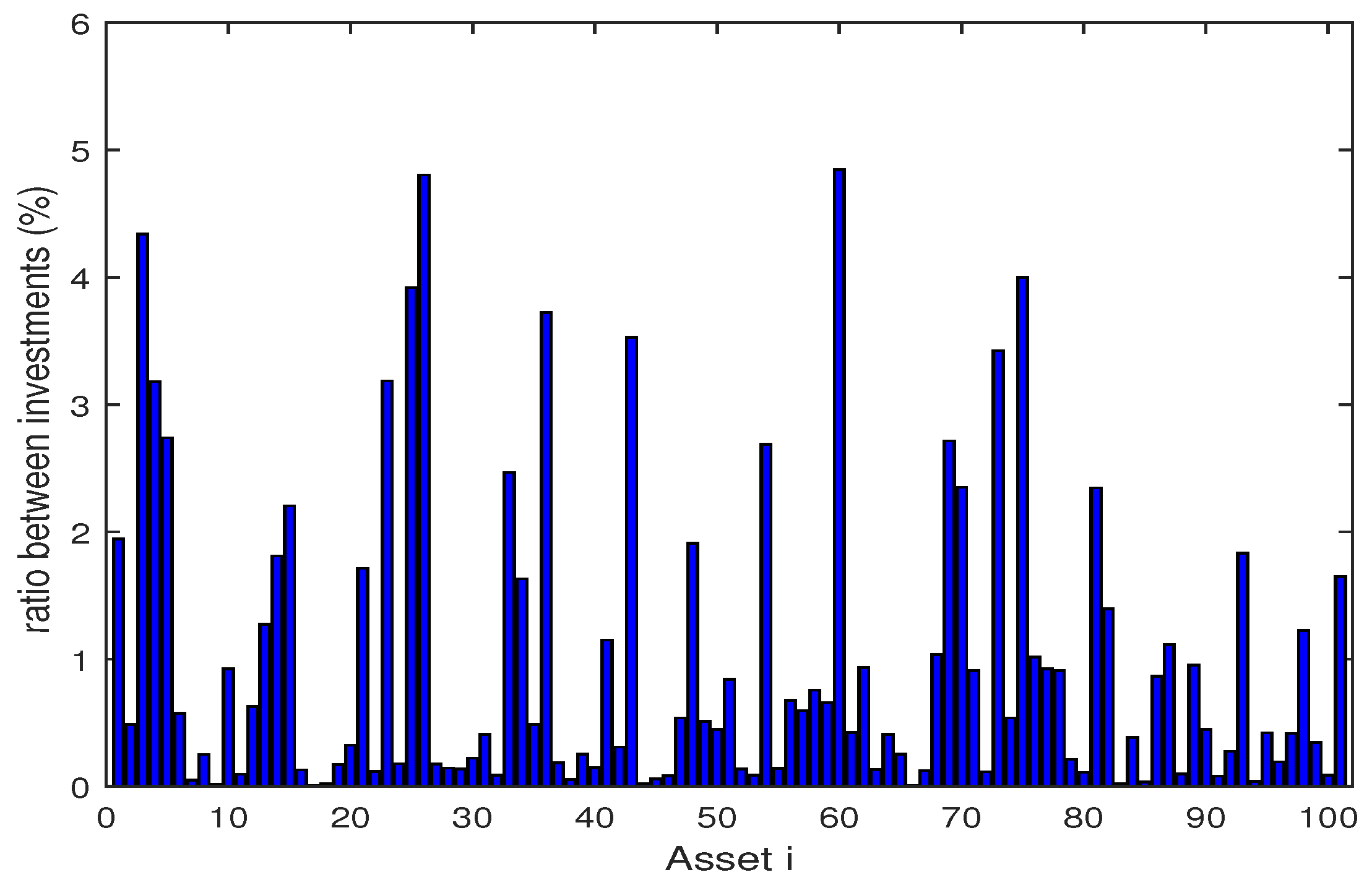
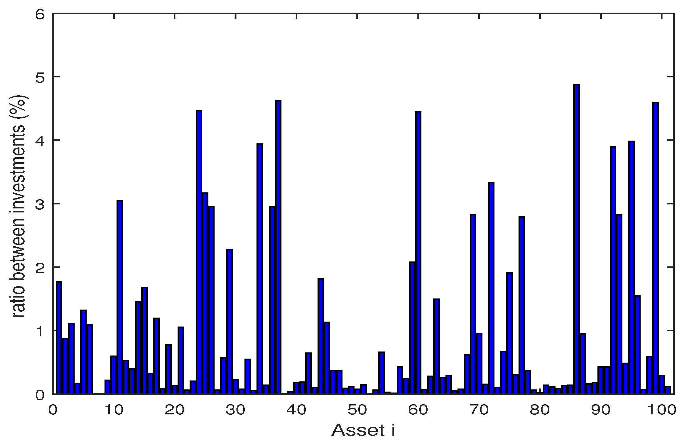
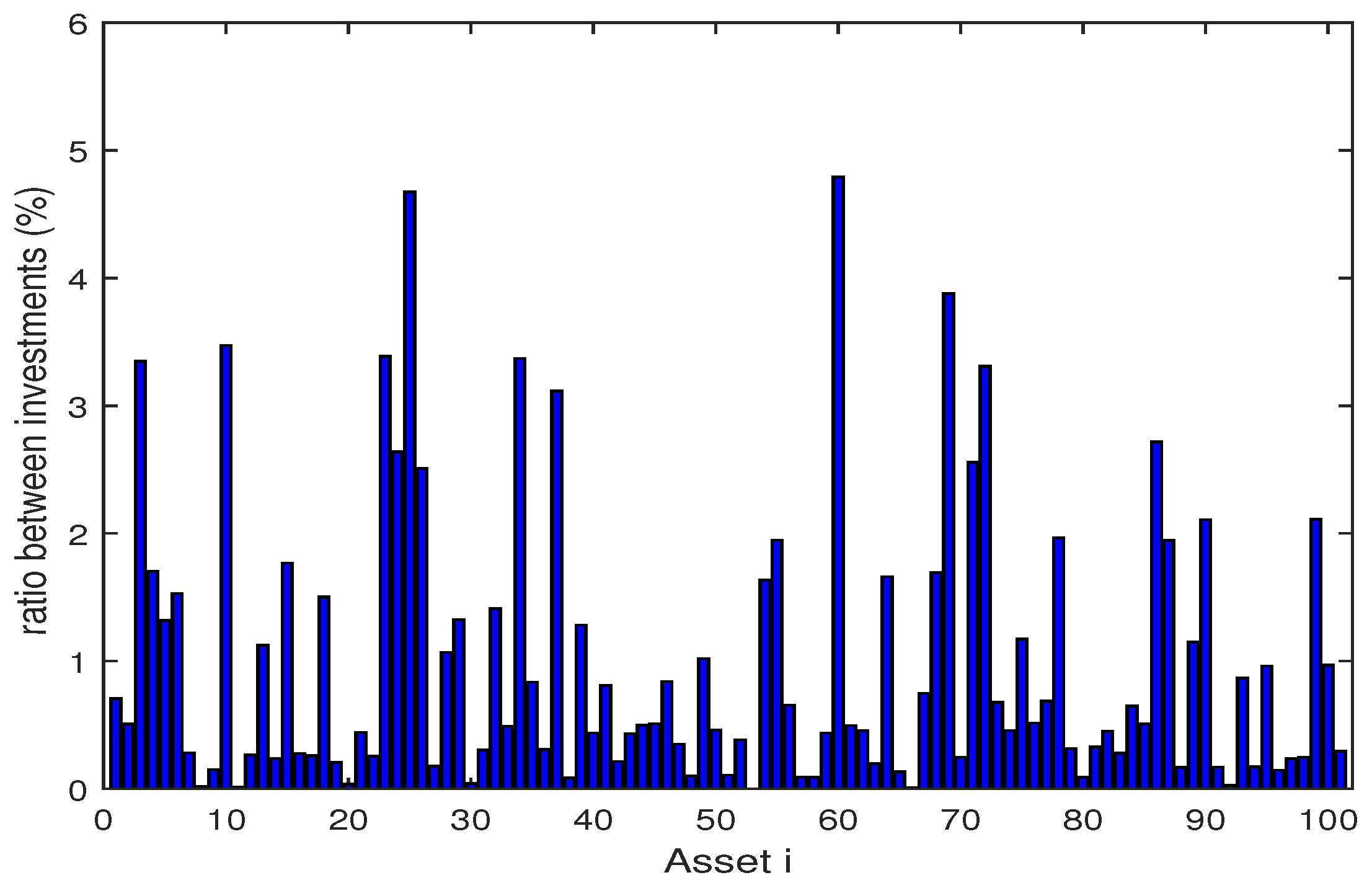
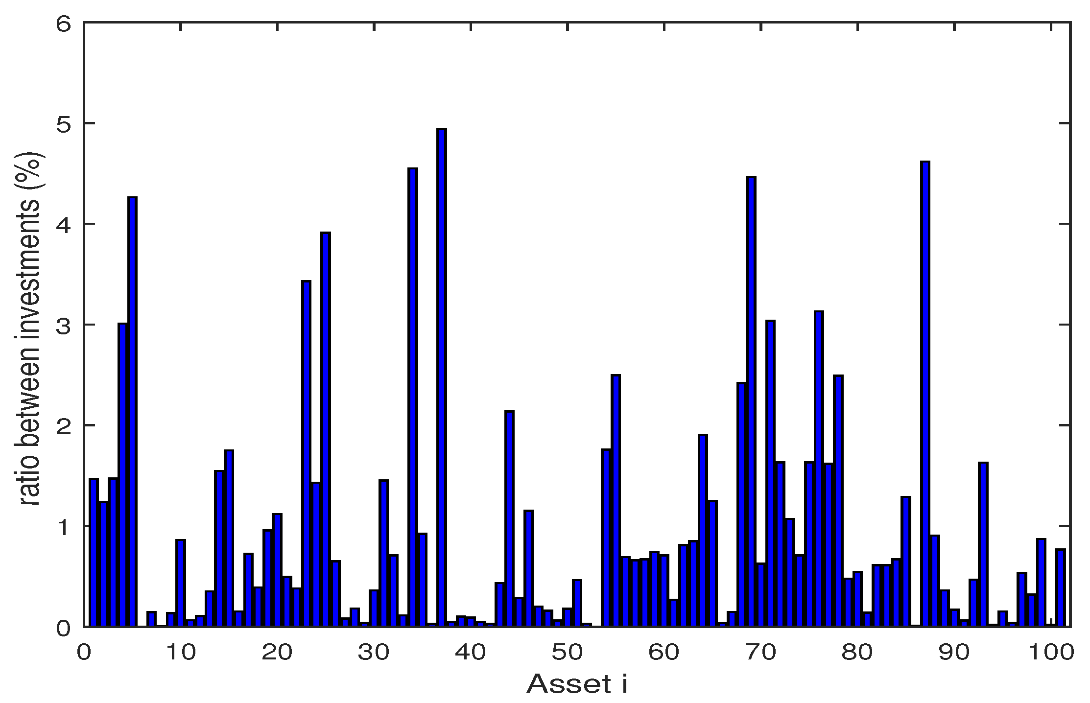
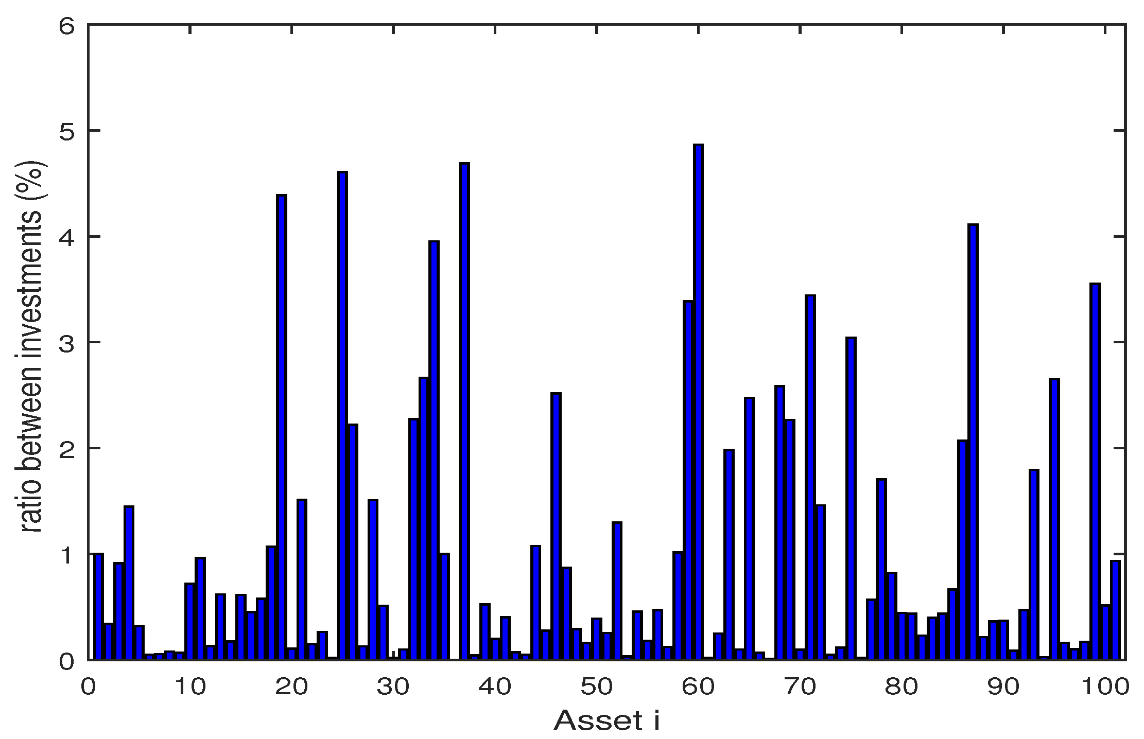
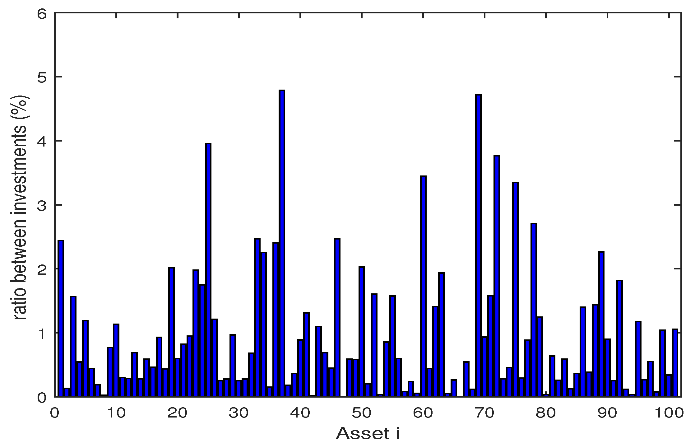
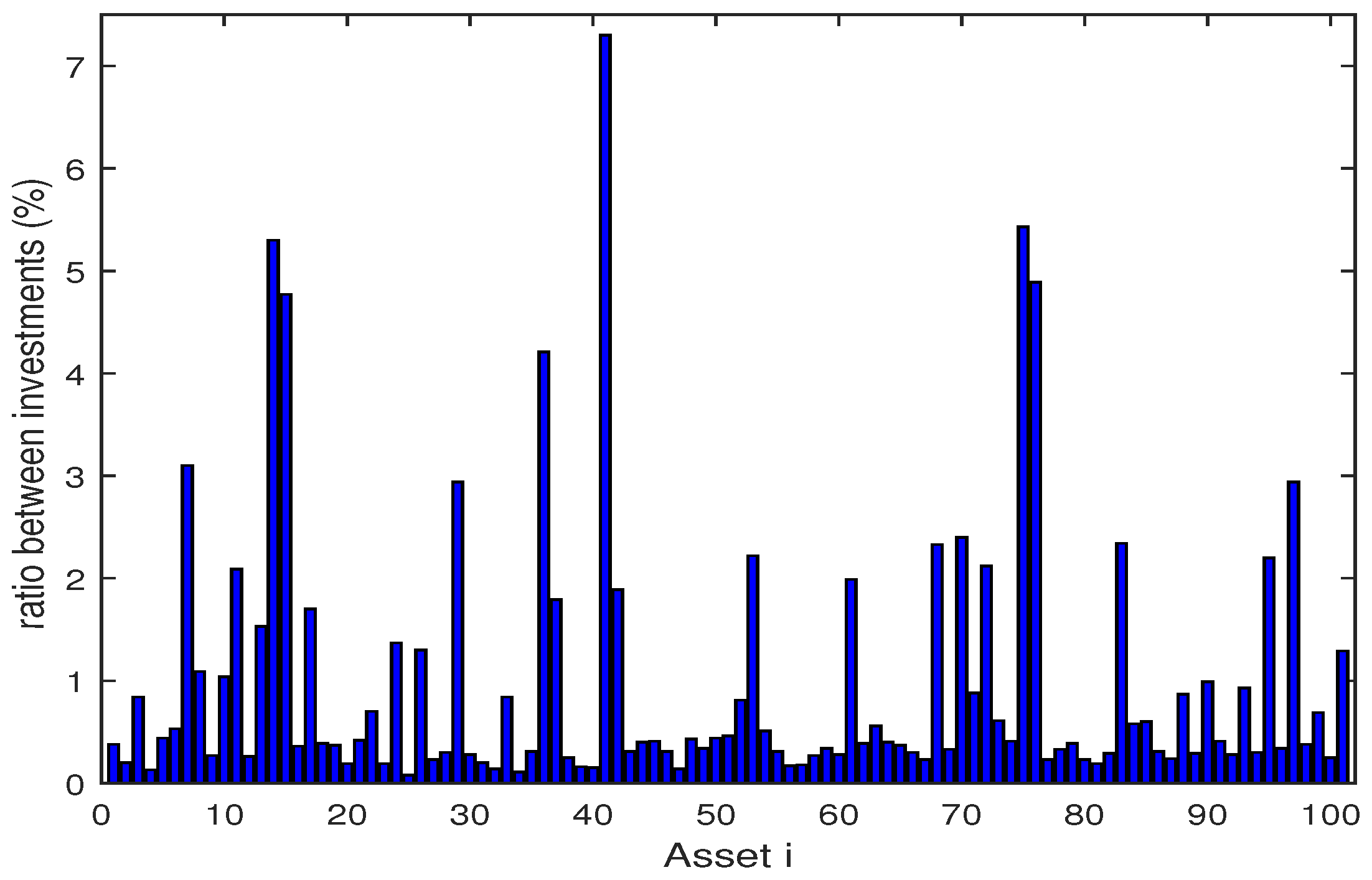
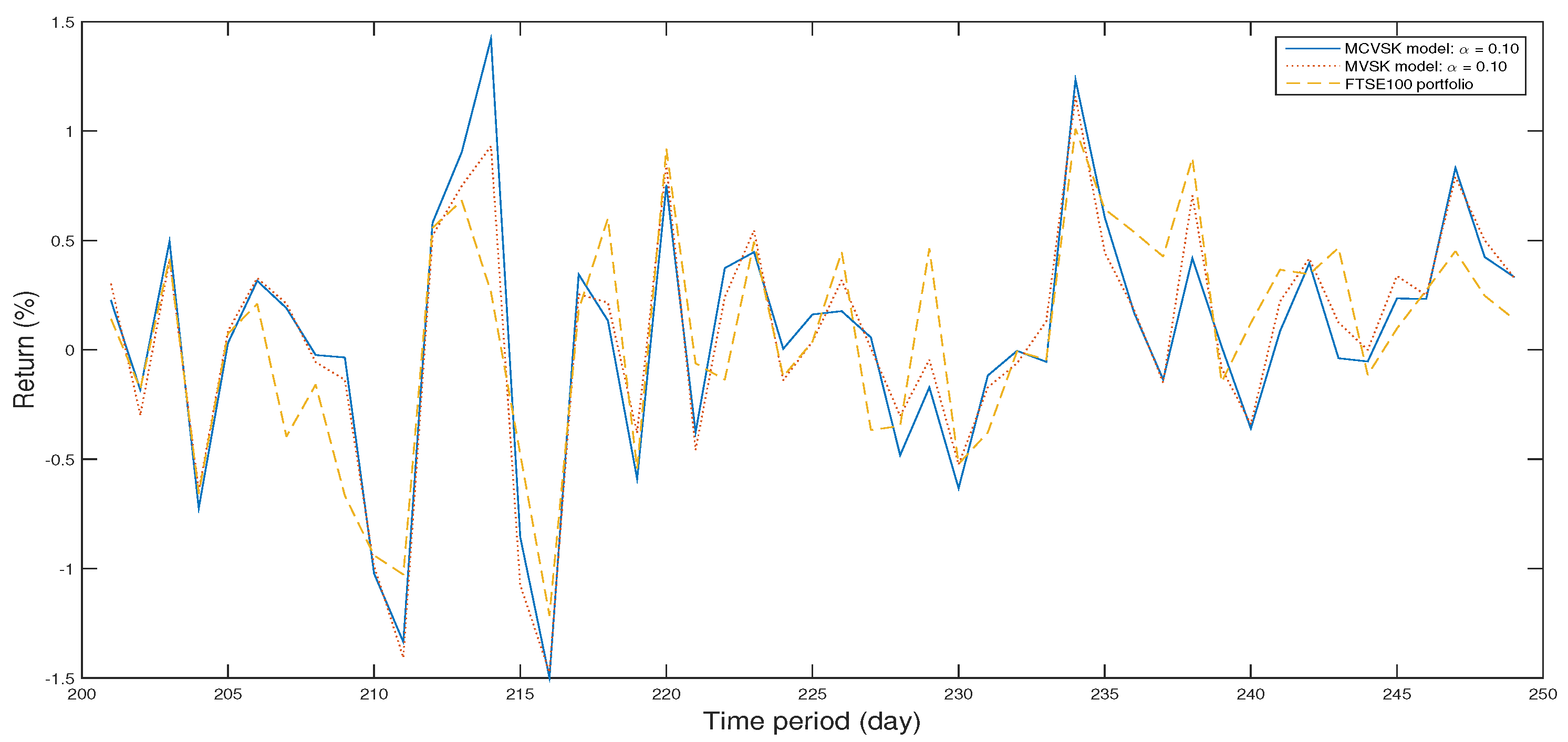
The Figure 2, Figure 3, Figure 4, Figure 5, Figure 6, Figure 7, Figure 8, Figure 9, Figure 10 and Figure 11 show the specific asset structure of optimal portfolio and the return to optimal portfolio in each period by GWO algorithm. Specifically speaking, Figure 2, Figure 3, Figure 4, Figure 5, Figure 6 and Figure 7 show the specific asset composition of the portfolio optimized by GWO algorithm and there are a total of 101 assets that can be invested in each portfolio. Figure 8 shows the specific asset composition of the FTSE100 index portfolio. Figure 9, Figure 10 and Figure 11 show the return of optimal portfolio by model (33) and model (34) in each period by GWO algorithm and the FTSE100 Index portfolio in backtesting with three kinds of confidence levels. Among them, the data set for the backtesting is the historical rate of return for the previous 200 days, which is the x-axis scale in Figure 9, Figure 10 and Figure 11.
In the above, we set up a backtest which compares the optimal portfolio obtained from MCVSK model and MVSK model by GWO algorithm, PSO algorithm and GA with FTSE100 index. Furthermore, we set up an out-of-sample test to evaluate the performance of the selected portfolio over the remaining 49 samples. The Figure 12, Figure 13 and Figure 14 show the return of optimal portfolio in another 49 days.
4.2. Numerical Analysis
In the above experiment, we conduct in-sample test and out-of-sample test of MCVSK and MVSK portfolio optimization models by GWO algorithm, PSO algorithm and GA respectively, then we compare them with FTSE100 index and the control group y. In this section, we mainly consider four indicators: skewness, kurtosis, VaR or CVaR and . From the results of backtesting, it’s shown that the skewness of portfolio derived from MCVSK and MVSK model are higher than FTSE100 index and control group y. Simultaneously, its value of kurtosis is rather lower than FTSE100 index and control group y. On the indicator of risk measure, MCVSK model take CVaR as risk measure while MVSK model’s risk measure is VaR. It can be seen from the experimental results that the portfolio optimized by GWO algorithm are generally much more profitable than FTSE100 index and control group y while having lower risks.
Specifically speaking, when the confidence coefficient is 1%, 5% or 10%, the CVaR of portfolio obtained by MCVSK model is −2.7743, −2.1648 and −1.7413 respectively, which is lower than −3.2503, −2.3205 and −1.8086. At the same time, the return of portfolio obtained by MCVSK model is 0.1430, 0.1478 and 0.1512 respectively, which is greatly higher than 0.1017. Compare the MCVSK model with the MVSK model, it can be found that portfolio obtained by MCVSK model generally has a better performance than MVSK model on the rate of return indicator. Specifically speaking, when the confidence coefficient is 1%, the return of portfolio obtained by MCVSK model is 0.1430 while the portfolio obtained by MVSK model is 0.1402. When the confidence coefficient is 5% and 10%, there is also the same phenomenon. Therefore, in a sense, CVaR has its special advantage as a type of risk measure.
Then we compare the GWO algorithm with PSO algorithm and GA. From the experimental results, it can be seen that all three algorithms can obtain excess returns when all the constraints on the portfolio optimization model are met. However, as a main evaluation index, the return to portfolio optimized by GWO algorithm is much higher than that of PSO algorithm and GA. Specifically speaking, when the confidence level is 1%, the GWO algorithm optimizes the MCVSK model to obtain a return on portfolio of 0.1430. Under the same conditions, the PSO algorithm optimizes the return on portfolio to 0.1107 and GA to 0.1215. This phenomenon also exists when the confidence level is 5% and 10%. While having a higher rate of return, the risk of portfolio optimized by GWO algorithm is similar to the portfolios optimized by PSO algorithm or GA. This shows that the GWO algorithm has a higher optimization capability in optimizing the MCVSK and MVSK portfolio optimization model.
From the results of out-of-sample tests, the MCVSK model and MVSK model optimized by GWO algorithm also have a wonderful performance. Generally speaking, the experimental results prove that the GWO algorithm has great potential in solving single-objective portfolio optimization problems. The GWO algorithm not only has a faster optimization speed, but also maintains a high optimization quality. It’s believed that GWO algorithm will have a much wider application.
5. Conclusions and Future Research
In this paper, we introduce several constraints, including skewness and kurtosis, into the basic second-order stochastic dominance portfolio optimization model. Besides, we use two different risk measures in the model, which we call them MCVSK model and MVSK model. As a single-objective optimization model, the portfolio optimized by GWO algorithm can achieve more return than PSO algorithm, GA and FTSE100 index from the experimental results. We also find that, compared with using VAR as risk measure, using CVAR as risk measure can achieve better and more stable performance. Generally speaking, the GWO algorithm can get a better portfolio faster, which shows the excellent optimization ability and optimization efficiency of the GWO algorithm. It is believed that GWO algorithm has great potential in solving portfolio optimization problem.
As a single-objective optimization model, MCVSK model and MVSK model only take return as one and only optimization goal. Therefore, the portfolio optimized by MCVSK model or MVSK model will have a higher risk than FTSE100 index, which means the portfolio obtained by MCVSK model and MVSK model will not meet the specific risk appetite of all investors. In the future, we will try to discuss the multiple objective portfolio optimization model based on second-order stochastic dominance constraint, which is designed to make up for the shortcomings in the single-objective portfolio optimization model. Moreover, From the result of experiment, we find that the efficiency of the model is closely related to the choice of benchmark. Therefore, we will pay attention to this problem in the following research.
Author Contributions
Tao Ye and Siling Feng contributed the new processing method, conceived and designed the experiments; Yixuan Ren performed the experiments; Tao Ye analyzed the data; Yixuan Ren wrote the Section 3 and Tao Ye wrote the rest of paper; Mengxing Huang contributed analysis tools.
Acknowledgments
We gratefully acknowledge the support of the Young Talents’ Science and Technology Innovation Project of Hainan Association for Science and Technology (No. QCXM201806), the Joint Funds of the National Natural Science Foundation of China (No. 61462022, No. 11561017, No. 11601108), Major Science and Technology Project of Hainan Province (ZDKJ2016015) in carrying out this research.
Conflicts of Interest
The authors declare no conflict of interest.
Abbreviations
The following abbreviations are used in this manuscript:
| GWO | Gray Wolf Optimization |
| PSO | Particle Swarm Optimization |
| GA | Genetic Algorithm |
| MV | Mean-Variance |
| MAD | Mean Absolute Deviation |
| VaR | Value at Risk |
| CVaR | Conditional Value at Risk |
| SD | Stochastic Dominance |
| FSD | First-Order Stochastic Dominance |
| SSD | Second-Order Stochastic Dominance |
| ASD | Almost Stochastic Dominance |
| MVS | Mean-Variance-Skewness |
| MOEAs | Multi-Objective Evolutionary Algorithms |
| NSGA-II | Non-Dominated Sorting Genetic Algorithm II |
| SPEA-II | Strength Parato Evolutionary Algorithm II |
| MCVSK | Mean-CVaR-skewness-kurtosis |
| MVSK | Mean-VaR-skewness-kurtosis |
| IPSO | Immune Particle Swarm Optimization |
| ACA | Ant Colony Algrothrim |
| BBO | Biogeography-based Optimization |
| CNN | Convolutional Neural Network |
| LSSVM | Least Squares Support Vector Machine |
Appendix A

Table A1.
The specific index weight data of FTSE100 Index.
| Constitution | Index Weight (%) | Constitution | Index Weight (%) |
|---|---|---|---|
| 3i Group | 0.38 | Admiral Group | 0.2 |
| Anglo American | 0.84 | Antofagasta | 0.13 |
| Ashtead Group | 0.44 | Associated British Foods | 0.53 |
| AstraZeneca | 3.1 | Aviva | 1.09 |
| Babcock International Group | 0.27 | BAE Systems | 1.04 |
| Barclays | 2.09 | Barratt Developments | 0.26 |
| BHP Billition | 1.53 | BP | 5.3 |
| British American Tobacco | 4.77 | British Land Co | 0.36 |
| BT Group | 1.7 | Bunzl | 0.39 |
| Burberry Group | 0.37 | Capita | 0.19 |
| Carnival | 0.42 | Centrica | 0.7 |
| Coca-Cola HBC AG | 0.19 | Compass Group | 1.37 |
| ConvaTec Group | 0.08 | CRH | 1.3 |
| Croda International | 0.23 | DCC | 0.3 |
| Diageo | 2.94 | Direct Line Insurance Group | 0.28 |
| Dixons Carphone | 0.2 | Easyjet | 0.14 |
| Experian | 0.84 | Fresnillo | 0.11 |
| GKN | 0.31 | GlaxoSmithKline | 4.21 |
| Glencore | 1.79 | Hammerson | 0.25 |
| Hargreaves Lansdown | 0.16 | Hikma Pharmaceuticals | 0.15 |
| HSBC HIdgs | 7.3 | Imperial Brands | 1.89 |
| Informa | 0.31 | InterContinental Hotels Group | 0.4 |
| International Consolidated Airlines Group | 0.41 | Intertek Group | 0.31 |
| Intu Properties | 0.14 | ITV | 0.43 |
| Johnson Matthey | 0.34 | Kingfisher | 0.44 |
| Land Securities Group | 0.46 | Legal & General Group | 0.81 |
| LIoyds Banking Group | 2.22 | London Stock Exchange Group | 0.51 |
| Marks & Spencer Group | 0.31 | Mediclinic International pIc | 0.17 |
| Merlin Entertainments | 0.18 | Micro Focus International | 0.27 |
| Mondi | 0.34 | Morrison (Wm) Supermarkets | 0.28 |
| National Grid | 1.99 | Next | 0.39 |
| Old Mutual | 0.56 | Paddy Power Betfair | 0.4 |
| Pearson | 0.37 | Persimmon | 0.3 |
| Provident Financial | 0.23 | Prudential | 2.33 |
| Randgold Resources | 0.33 | Reckitt Benckiser Group | 2.4 |
| RELX | 0.88 | Rio Tinto | 2.12 |
| Rolls-Royce Holdings | 0.61 | Royal Bank Of Scotland Group | 0.41 |
| Royal Dutch Shell A | 5.43 | Royal Dutch Shell B | 4.89 |
| Royal Mail | 0.23 | RSA Insurance Group | 0.33 |
| Sage Group | 0.39 | Sainsbury (J) | 0.23 |
| Schroders | 0.19 | Severn Trent | 0.29 |
| Shire | 2.34 | Sky | 0.58 |
| Smith & Nephew | 0.6 | Smiths Group | 0.31 |
| Smurfit Kappa Group | 0.24 | SSE | 0.87 |
| St. James’s Place | 0.29 | Standard Chartered | 0.99 |
| Standard Life | 0.41 | Taylor Wimpey | 0.28 |
| Tesco | 0.93 | TUI AG | 0.3 |
| Unilever | 2.2 | United Utilities Group | 0.34 |
| Vodafone Group | 2.94 | Whitbread | 0.38 |
| Wolseley | 0.69 | Worldpay Group | 0.25 |
| WPP | 1.29 |
References
- Markowitz, H.M. Portfolio Selection. J. Financ. 1952, 7, 77–91. [Google Scholar]
- Markowitz, H.M. Portfolio Selection: Efficient Diversification of Investments; John Wiley and Sons: New York, NY, USA, 1959. [Google Scholar]
- Lwin, K.T.; Qu, R.; MacCarthy, B.L. Mean-VaR portfolio optimization: A nonparametric approach. Eur. J. Oper. Res. 2017, 260, 751–766. [Google Scholar] [CrossRef]
- Chunhachinda, P.; Dandapani, K.; Hamid, S.; Prakash, A.J. Portfolio selection and skewness: Evidence from international stock markets. J. Bank. Financ. 1997, 21, 143–167. [Google Scholar] [CrossRef]
- Markowitz, H.; Todd, P.; Xu, G.; Yamane, Y. Computation of mean-semivariance efficient sets by the critical line algorithm. Ann. Oper. Res. 1993, 45, 307–317. [Google Scholar] [CrossRef]
- Konno, H.; Yamazaki, H. Mean-Absolute Deviation Portfolio Optimization Model and Its Applications to Tokyo Stock Market. Manag. Sci. 1991, 37, 519–531. [Google Scholar] [CrossRef]
- Speranza, G.M. Linear Programming Models for Portfolio Optimization. Finance 1993, 14, 107–123. [Google Scholar]
- Zhou, K.; Gao, J.; Li, D.; Cui, X. Dynamic mean—VaR portfolio selection in continuous time. Quant. Financ. 2017, 17, 1631–1643. [Google Scholar] [CrossRef]
- Artzner, P.; Delbaen, F.; Eber, J.M.; Heath, D. Coherent measures of risk. Math. Financ. 1999, 9, 203–228. [Google Scholar] [CrossRef]
- Fishburn, P.C. Mean-Risk Analysis with Risk Associated with Below-Target Returns. Am. Econ. Rev. 1975, 67, 116–126. [Google Scholar]
- Dentcheva, D.; Ruszczyński, A. Portfolio optimization with stochastic dominance constraints. J. Bank. Financ. 2006, 30, 433–451. [Google Scholar] [CrossRef]
- Leshno, M.; Levy, H. Preferred by “All” and Preferred by “Most” Decision Makers: Almost Stochastic Dominance. Manag. Sci. 2002, 48, 1074–1085. [Google Scholar] [CrossRef]
- Javanmardi, L.; Lawryshyn, Y. A new rank dependent utility approach to model risk averse preferences in portfolio optimization. Ann. Oper. Res. 2016, 237, 161–176. [Google Scholar] [CrossRef]
- Arditti, F.D. Risk and the Required Return on Equity. J. Financ. 1967, 22, 19–36. [Google Scholar] [CrossRef]
- Yu, L.; Wang, S.; Lai, K.K. Neural network-based mean–variance–skewness model for portfolio selection. Comput. Oper. Res. 2008, 35, 34–46. [Google Scholar] [CrossRef]
- Bhattacharyya, R.; Kar, S.; Majumder, D.D. Fuzzy Mean-Variance-skewness portfolio selection models by interval analysis. Comput. Math. Appl. 2011, 61, 126–137. [Google Scholar] [CrossRef]
- Pouya, A.R.; Solimanpur, M.; Rezaee, M.J. Solving multi-objective portfolio optimization problem using invasive weed optimization. Swarm. Evol. Comput. 2016, 28, 42–57. [Google Scholar] [CrossRef]
- Soleimani, H.; Golmakani, H.R.; Salimi, M.H. Markowitz-based portfolio selection with minimum transaction lots, cardinality constraints and regarding sector capitalization using genetic algorithm. Expert. Syst. Appl. 2009, 36, 5058–5063. [Google Scholar] [CrossRef]
- Macedo, L.L.; Godinho, P.; Alves, M.J. Mean-Semivariance Portfolio Optimization with Multiobjective Evolutionary Algorithms and Technical Analysis Rules. Expert. Syst. Appl. 2017, 79, 33–43. [Google Scholar] [CrossRef]
- Lai, T.Y. Portfolio selection with skewness: A multiple-objective approach. Rev. Quant. Financ. Account. 1991, 1, 293–305. [Google Scholar] [CrossRef]
- Chen, W.; Wang, Y.; Zhang, J.; Lu, S. Uncertain portfolio selection with high-order moments. J. Intell. Fuzzy. Syst. 2017, 33, 1–15. [Google Scholar] [CrossRef]
- Mirjalili, S.; Mirjalili, S.M.; Lewis, A. Grey wolf optimizer. Adv. Eng. Softw. 2014, 69, 46–61. [Google Scholar] [CrossRef]
- Wang, S.; Li, P.; Chen, P.; Phillips, P.; Liu, G.; Du, S.; Zhang, Y. Pathological brain detection via wavelet packet tsallis entropy and real-coded biogeography-based optimization. Fund. Inform. 2017, 151, 275–291. [Google Scholar] [CrossRef]
- Zhang, Y.D.; Zhang, Y.; Lv, Y.D.; Hou, X.X.; Liu, F.Y.; Jia, W.J.; Yang, M.M.; Phillips, P.; Wang, S.H. Alcoholism detection by medical robots based on Hu moment invariants and predator–prey adaptive-inertia chaotic particle swarm optimization. Comput. Electr. Eng. 2017, 63, 126–138. [Google Scholar] [CrossRef]
- Kumaran, N.; Vadivel, A.; Kumar, S.S. Recognition of human actions using CNN-GWO: A novel modeling of CNN for enhancement of classification performance. Mutimed. Tools Appl. 2018, 1, 1–33. [Google Scholar] [CrossRef]
- Mustaffa, Z.; Sulaiman, M.H.; Kahar, M.N.M. Training LSSVM with GWO for price forecasting. Electron. Vis. 2015, 1–6. [Google Scholar] [CrossRef]
- Zhang, H.W.; Yu, H.S.; Pang, L.P.; Wang, J.H. Solution to constrained optimization problem of second order stochastic dominance by gentic algorithm. J. Dalian Univ. Technol. 2016, 56, 299–303. [Google Scholar]
- Pflug, G.C. Some Remarks on the Value-at-Risk and the Conditional Value-at-Risk; Probabilistic Constrained Optimization; Springer: Boston, MA, USA, 2000; pp. 272–281. [Google Scholar]
- Rockafellar, R.T.; Uryasev, S. Conditional value-at-risk for general loss distributions. J. Bank. Financ. 2002, 26, 1443–1471. [Google Scholar] [CrossRef]
- Rockafellar, R.T.; Uryasev, S. Optimization of conditional value-at-risk. J. Risk. 2000, 2, 21–42. [Google Scholar] [CrossRef]
- Ye, T.; Yang, Z.; Feng, S. Biogeography-Based Optimization of the Portfolio Optimization Problem with Second Order Stochastic Dominance Constraints. Algorithms 2017, 10, 100. [Google Scholar] [CrossRef]
- Kallio, M.; Hardoroudi, N.D. Second-order Stochastic Dominance Constrained Portfolio Optimization: Theory and Computational Tests. Eur. J. Oper. Res. 2017, 264, 675–685. [Google Scholar] [CrossRef]
- Fábián, C.I.; Mitra, G.; Roman, D. Processing second-order stochastic dominance models using cutting-plane representations. Math. Program. 2011, 130, 33–57. [Google Scholar] [CrossRef]
- Ogryczak, W.; Ruszczyński, A. From stochastic dominance to mean-risk models: Semideviations as risk measures. Eur. J. Oper. Res. 1999, 116, 33–50. [Google Scholar] [CrossRef]
- Noyan, N.; Rudolf, G. Optimization with Multivariate Conditional Value-at-Risk Constraints. Oper. Res. 2013, 61, 990–1013. [Google Scholar] [CrossRef] [Green Version]
- Yoshimoto, A. The mean-variance approach to portfolio optimization subject to transaction costs. J. Oper. Res. Soc. Jpn. 1996, 39, 99–117. [Google Scholar] [CrossRef]
- Bhattacharyya, R.; Chatterjee, A.; Kar, S. Uncertainty theory based multiple objective mean-entropy-skewness stock portfolio selection model with transaction costs. J. Uncertain. Anal. Appl. 2013, 1, 16. [Google Scholar] [CrossRef]
- Lobo, M.S.; Fazel, M.; Boyd, S. Portfolio optimization with linear and fixed transaction costs. Ann. Oper. Res. 2007, 152, 341–365. [Google Scholar] [CrossRef]
- Zawbaa, H.M.; Emary, E.; Grosan, C.; Snasel, V. Large-dimensionality small-instance set feature selection: A hybrid bio-inspired heuristic approach. Swarm. Evol. Comput. 2018. [Google Scholar] [CrossRef]
Figure 1.
The procedure chat of the GWO algorithm.

Figure 2.
The specific asset structure of optimal portfolio in of model (33) for 101 assets by GWO algorithm.
Figure 2.
The specific asset structure of optimal portfolio in of model (33) for 101 assets by GWO algorithm.

Figure 3.
The specific asset structure of optimal portfolio in of model (33) for 101 assets by GWO algorithm.
Figure 3.
The specific asset structure of optimal portfolio in of model (33) for 101 assets by GWO algorithm.

Figure 4.
The specific asset structure of optimal portfolio in of model (33) for 101 assets by GWO algorithm.
Figure 4.
The specific asset structure of optimal portfolio in of model (33) for 101 assets by GWO algorithm.

Figure 5.
The specific asset structure of optimal portfolio in of model (34) for 101 assets by GWO algorithm.
Figure 5.
The specific asset structure of optimal portfolio in of model (34) for 101 assets by GWO algorithm.

Figure 6.
The specific asset structure of optimal portfolio in of model (34) for 101 assets by GWO algorithm.
Figure 6.
The specific asset structure of optimal portfolio in of model (34) for 101 assets by GWO algorithm.

Figure 7.
The specific asset structure of optimal portfolio in of model (34) for 101 assets by GWO algorithm.
Figure 7.
The specific asset structure of optimal portfolio in of model (34) for 101 assets by GWO algorithm.

Figure 8.
The specific asset structure of FTSE100 index portfolio for 101 assets.

Figure 9.
The return of optimal portfolio by model (33) in each period with model (34) by GWO algorithm and the FTSE100 Index portfolio in backtesting with .

Figure 10.
The return of optimal portfolio by model (33) in each period with model (34) by GWO algorithm and the FTSE100 Index portfolio in backtesting with .

Figure 11.
The return of optimal portfolio by model (33) in each period with model (34) by GWO algorithm and the FTSE100 Index portfolio in backtesting with .

Figure 12.
The return of optimal portfolio by model (33) in each period with model (34) by GWO algorithm and the FTSE100 Index portfolio in out-of-sample test with .

Figure 13.
The return of optimal portfolio by model (33) in each period with model (34) by GWO algorithm and the FTSE100 Index portfolio in out-of-sample test with .

Figure 14.
The return of optimal portfolio by model (33) in each period with model (34) by GWO algorithm and the FTSE100 Index portfolio in out-of-sample test with .

Table 1.
The results of Backtesting.
| Algorithm | Skew | Kurt | VaR | CVaR | E [g(x,)] | Max | Time (s) | ||
|---|---|---|---|---|---|---|---|---|---|
| MCVSK | 0.01 | GWO | 0.1726 | 4.0974 | −2.2535 | −2.7743 | 0.1430 | 0.0484 | 30.77 |
| PSO | 0.0878 | 3.9355 | −2.3300 | −2.7368 | 0.1107 | 0.0389 | 27.77 | ||
| GA | 0.1307 | 3.8451 | −2.2777 | −2.7744 | 0.1215 | 0.0378 | 28.59 | ||
| 0.05 | GWO | 0.0734 | 3.8483 | −1.7844 | −2.1648 | 0.1478 | 0.0488 | 24.94 | |
| PSO | 0.0292 | 4.0188 | −1.5916 | −2.2091 | 0.1109 | 0.0369 | 32.45 | ||
| GA | 0.1362 | 4.0364 | −1.7264 | −2.1502 | 0.1282 | 0.0386 | 30.20 | ||
| 0.10 | GWO | 0.2033 | 3.8933 | −1.1009 | −1.7413 | 0.1512 | 0.0479 | 32.12 | |
| PSO | 0.0346 | 3.9227 | −1.0638 | −1.7982 | 0.1110 | 0.0349 | 30.07 | ||
| GA | 0.2087 | 3.9117 | −1.1509 | −1.7554 | 0.1210 | 0.0356 | 27.47 | ||
| MVSK | 0.01 | GWO | 0.3197 | 3.9699 | −2.1251 | −2.6291 | 0.1402 | 0.0494 | 30.12 |
| PSO | 0.0934 | 3.8752 | −2.4055 | −2.8165 | 0.1117 | 0.0353 | 31.21 | ||
| GA | 0.0898 | 3.9745 | −2.2682 | −2.7807 | 0.1228 | 0.0366 | 27.47 | ||
| 0.05 | GWO | 0.2464 | 4.1137 | −1.6823 | −2.0712 | 0.1451 | 0.0487 | 28.60 | |
| PSO | 0.1575 | 3.9913 | −1.7283 | −2.1363 | 0.1347 | 0.0423 | 27.77 | ||
| GA | 0.1324 | 3.9691 | −1.7344 | −2.1379 | 0.1215 | 0.0359 | 23.86 | ||
| 0.10 | GWO | 0.1880 | 4.1003 | −1.1198 | −1.7461 | 0.1393 | 0.0479 | 26.73 | |
| PSO | 0.0440 | 3.9591 | −0.9915 | −1.7541 | 0.1064 | 0.0333 | 26.81 | ||
| GA | 0.1612 | 3.9245 | 1.1932 | 1.7606 | 0.1261 | 0.0341 | 26.02 | ||
| FTSE100 | 0.01 | × | 0.0151 | 4.3361 | −2.6739 | −3.2503 | 0.1017 | 0.0730 | × |
| 0.05 | −1.5442 | −2.3205 | |||||||
| 0.10 | −1.1953 | −1.8086 | |||||||
| y | 0.01 | × | −0.1992 | 4.6663 | −3.1508 | −3.2600 | 0.0612 | 0.0099 | × |
| 0.05 | −1.6022 | −2.4337 | |||||||
| 0.10 | −1.0599 | −1.8505 |
© 2018 by the authors. Licensee MDPI, Basel, Switzerland. This article is an open access article distributed under the terms and conditions of the Creative Commons Attribution (CC BY) license (http://creativecommons.org/licenses/by/4.0/).
Share and Cite
MDPI and ACS Style
Ren, Y.; Ye, T.; Huang, M.; Feng, S. Gray Wolf Optimization Algorithm for Multi-Constraints Second-Order Stochastic Dominance Portfolio Optimization. Algorithms 2018, 11, 72. https://doi.org/10.3390/a11050072
AMA Style
Ren Y, Ye T, Huang M, Feng S. Gray Wolf Optimization Algorithm for Multi-Constraints Second-Order Stochastic Dominance Portfolio Optimization. Algorithms. 2018; 11(5):72. https://doi.org/10.3390/a11050072
Chicago/Turabian StyleRen, Yixuan, Tao Ye, Mengxing Huang, and Siling Feng. 2018. "Gray Wolf Optimization Algorithm for Multi-Constraints Second-Order Stochastic Dominance Portfolio Optimization" Algorithms 11, no. 5: 72. https://doi.org/10.3390/a11050072
Note that from the first issue of 2016, this journal uses article numbers instead of page numbers. See further details here.