A Modified Artificial Bee Colony Algorithm Based on the Self-Learning Mechanism

Abstract

Artificial bee colony (ABC) algorithm, a novel category of bionic intelligent optimization algorithm, was achieved for solving complex nonlinear optimization problems. Previous studies have shown that ABC algorithm is competitive to other biological-inspired optimization algorithms, but there still exist several insufficiencies due to the inefficient solution search equation (SSE), which does well in exploration but poorly in exploitation. To improve accuracy of the solutions, this paper proposes a modified ABC algorithm based on the self-learning mechanism (SLABC) with five SSEs as the candidate operator pool; among them, one is good at exploration and two of them are good at exploitation; another SSE intends to balance exploration and exploitation; moreover, the last SSE with Lévy flight step-size which can generate smaller step-size with high frequency and bigger step-size occasionally not only can balance exploration and exploitation but also possesses the ability to escape from the local optimum. This paper proposes a simple self-learning mechanism, wherein the SSE is selected according to the previous success ratio in generating promising solutions at each iteration. Experiments on a set of 9 benchmark functions are carried out with the purpose of evaluating the performance of the proposed method. The experimental results illustrated that the SLABC algorithm achieves significant improvement compared with other competitive algorithms.

1. Introduction

In recent years, swarm intelligence algorithms have received a wide spread attention. The artificial bee colony (ABC) algorithm is a relatively new approach that was proposed by Karaboga [1,2], motivated by the collective foraging behavior of honey bees. In the process of foraging, the bees need to find the place of food source with the highest nectar amount. In ABC system, artificial bees search in the given search space and the food sources represent possible solutions for the optimisation problems. The bees update the candidate solutions by means of solution search equation (SSE) and if the new solution is better than the previous one in their memory, they memorize the new position and forget the previous one. Due to its simplicity and ease of implementation, the ABC algorithm has captured much attention and has been applied successfully to a variety of fields, such as classification and function approximation [3], feature selection [4], inverse modelling of a solar collector [5], electric power system optimization [6], multi-objective optimisation [7], complex network optimization [8], transportation energy demand [9], large-scale service composition for cloud manufacturing [10], job-shop scheduling problem with no-wait constraint [11], respiratory disease detection from medical images [12].

Although the ABC algorithm has been widely used in different fields, some researchers have also pointed out that the ABC algorithm suffers from low solution accuracy and poor convergence performance. To solve the optimization problem, the intelligent optimization algorithm should combine global search methods, used to locate the potential optimal regions, with local search methods, used to fine-tune the candidate solutions, to balance exploration and exploitation process. However, exploration strategies and exploitation strategies contradict each other and to achieve good performance, they should be well balanced. While the SSE of ABC, which is used to generate new candidate solutions based on the information of the present solutions, does well in exploration but poorly in exploitation, which results in the poor convergence rate. Thus, many related and improved ABC algorithms have been proposed [13,14,15,16].

Inspired by a operator of global best (gbest) solution in particle swarm optimization (PSO) algorithm [17], Zhu and Kwong proposed a modified ABC algorithm called gbest-guided ABC (GABC) algorithm to improve the exploitation [18]; the gbest term in the modified SSE can drive the new candidate solution towards the global best solution. Although the GABC algorithm accelerated the convergence rate, the exploration performance decreased. Therefore, how to balance exploration and exploitation has become the main goal in the ABC research. Inspired by differential evolution [19], Gao and Liu introduced a new initialization approach and proposed an improved SSE which is based on that the bee searches only around the best solution of the previous iteration to improve the exploitation; by hybridizing the original SSE and the improved SSE with the fixed selective probability, the new search mechanism obtains better performance [20]. After that, based on the two SSEs, Gao and Liu proposed the modified ABC (MABC) algorithm which excludes the onlooker and scout bee stage. In MABC, a selective probability was introduced to balance exploration of the original SSE and exploitation of the improved SSE [21]; if the new candidate solution obtained using the improved SSE is worse than the original one, the bee uses the original SSE to generate a new candidate solution with a certain probability. To well balance exploration and exploitation, Akay and Karaboga constructed an adaptive scaling factor (SF) which regulates the range of parameter in SSE by using Rechenberg’s 1/5 mutation rule; a smaller SF makes the candidate solution fine-tuned with a small steps while causing slow convergence rate and the bigger SF speeds up the search, but it reduces the exploitation performance [22]. In the original SSE in ABC algorithm, since the guidance of the last two term may be in opposite directions, it may cause an oscillation phenomenon. To overcome the oscillation phenomenon, Gao et al. presented a new SSE with two different candidate solutions selected from the solution space; moreover, an orthogonal learning strategy was developed to discover more effective information from the search experiences and to get more promising and efficient candidate solutions [23]. When the candidate solutions converge to the similar points, the SSE can cause a stagnation behavior during the search process, that means the value of the new candidate solution is the same with the value of the current solution. To overcome stagnation behavior of the algorithm, Babaoglu proposed a novel algorithm called distABC algorithm based on the distributed solution update rule, which uses the mean and standard deviation of the selected two solution to obtain a new candidate solution [24].

The above methods have achieved some progress, but there still exist some problems. The GABC algorithm improved the exploitation, but the exploration decreased. Even though MABC algorithm used two SSEs to balance exploration and exploitation, the selection mechanism and the fixed selective probability cannot adapt to the changing environment. Moreover, when the global best solution trapped in local optimum, GABC and MABC algorithm cannot escape from the local optimum effectively. The distABC algorithm overcame stagnation behavior, but distABC does poorly in exploitation. For population-based optimization methods, it is desirable to encourage the individuals to wander through the entire search space at the initial phase of the optimization; on the other hand, it is very important to fine-tune the candidate solutions in the succeeding phases of the optimization [25]. However, one SSE of original ABC algorithm cannot balance two aspects. Therefore, this paper proposes an achievable ABC algorithm which uses five SSEs as the candidate operator pool. The same with the SSE in ABC algorithm, the first SSE uses a solution selected randomly from the population to maintain population diversity and it emphasizes the exploration. Inspired by the PSO algorithm, the second SSE takes advantage of the information of the global best solution to guide the new candidate solution towards the global best solution. Therefore, the second SSE can improve the exploitation. To achieve good performance, the third SSE combines the above two SSEs which means that a randomly selected solution and the global best solution are all used in the SSE to balance exploration and exploitation. It seems that the global optimal solution is most likely around the best solution of the previous iteration. Therefore, the fourth SSE is the same with the one proposed in MABC algorithm which is based on that the bee searches only around the best solution of the previous iteration to improve the exploitation. When the candidate solutions trapped in local optimum, the above SSEs cannot escape from the local optimum effectively. To solve such problem, this paper proposes a novel SSE with Lévy flight step-size which can generate smaller step-size with high frequency and bigger step-size occasionally. The fifth SSE cannot only balance exploration and exploitation but also escape from the local optimum effectively. The five SSEs have both advantages and disadvantages and in order to make full use of the advantages of each SSE, this paper proposes a simple self-learning mechanism, wherein the SSE is selected according to the previous success ratio in generating promising solutions at each iteration. The SSE with a high success ratio means that the SSE can generate a better candidate solution with a large probability. Therefore, the self-learning mechanism cannot only select the appropriate SSE to generate new candidate solution but also adapt to the changing environment.

The following sections are organized as follows. Section 2 outlines the reviews of the classical ABC algorithm. Section 3 introduces the proposed self-learning mechanism (SLABC) algorithm. In Section 4, experiments are carried out to verify the effectiveness of SLABC algorithm based on nine benchmark functions in terms of t-test. Section 5 presents and discusses the experimental results. Finally, the conclusion is drawn in Section 6.

2. Classical ABC Algorithm

In the ABC algorithm, the colony of artificial bees contains three groups of bees: employed bees, onlooker bees and scouts bees [2]. Half of the colony consists of the employed bees, and another half consists of the onlooker bees. The scouts bees are transmuted from the inactive employed bees and then abandon their food source to search a new food source. Employed bees explore the food source in the search space and pass the food information to onlooker bees. Onlooker bees select the good food sources from those found by employed bees and further search the foods around the selected food source. The positions of the food sources are initialized in the search space and food sources present possible solutions for the optimization problem. There are $SN$ solutions, where $SN$ denotes the size of employed bees or onlooker bees. Suppose $x_i=\{x_{i,1},x_{i,2},\dots ,x_{i,D}\}$ is the position of the ith solution and D is the number of dimension to be optimized. The flow of ABC algorithm is shown as follows.

2.1. Employed Bee Stage

At this stage, each employed bee search around the given solution $x_i$ and let $v_i=x_i$. In the update process, the new candidate solution $v_i=\{v_{i,1},v_{i,2},\dots ,v_{i,D}\}$ is produced by using SSE as follows:

$$v_{i,j}=x_{i,j}+{\varphi }_{i,j}(x_{i,j}-x_{k,j})$$

(1)

where $k\in \{1,2,\dots ,SN\}$ and $j\in \{1,2,\dots ,D\}$ are randomly chosen indexes; k has to be different from i; ${\varphi }_{i,j}$ is a random number in the range $[-1,1]$. Then, a greedy selection mechanism is applied between $x_i$ and $v_i$ to select a better solution. After all the employed bees complete their searches, they share the solution information to the onlooker bees.

2.2. Onlooker Bee Stage

According to the fitness value of each solution, onlooker bees calculate the probability value $P_i$ associated with that solution,

$$P_i=\frac{{fit}_i}{{\sum }_{i=1}^{SN}{fit}_i}$$

(2)

where ${fit}_i$ is the fitness value of solution i and $SN$ is the number of solutions. Based on $P_i$ and roulette wheel selection method, an onlooker bee selects one solution to update. After selecting the solution $x_i$, the onlooker bee update it by using Equation (1) and the greedy selection mechanism is also used to select a better solution. At this stage, only the selected solution can be updated and the better solutions may be updated many times.

2.3. Scouts Bee Stage

If a solution cannot be improved further at least $limit$ times, this solution is assumed to be abandoned and a new solution will be produced randomly in the search space to replace the abandoned one. This operation can be defined as follows:

$$x_{i,j}=x_{min,j}+rand(0,1)(x_{max,j}-x_{min,j})$$

(3)

3. SLABC Algorithm

To improve the performance, the SLABC algorithm uses five SSEs as the candidate operator pool. One of the SSEs with Lévy flight step-size cannot only balance exploration and exploitation but also avoid trapping in the local optimum. This section first introduces the Lévy flight in detail.

3.1. Lévy Flight Step-Size

A Lévy flight is a random walk and the step-size satisfies a probability distribution which can be expressed as follows [26]:

$$P(s)=s^{-\lambda }$$

(4)

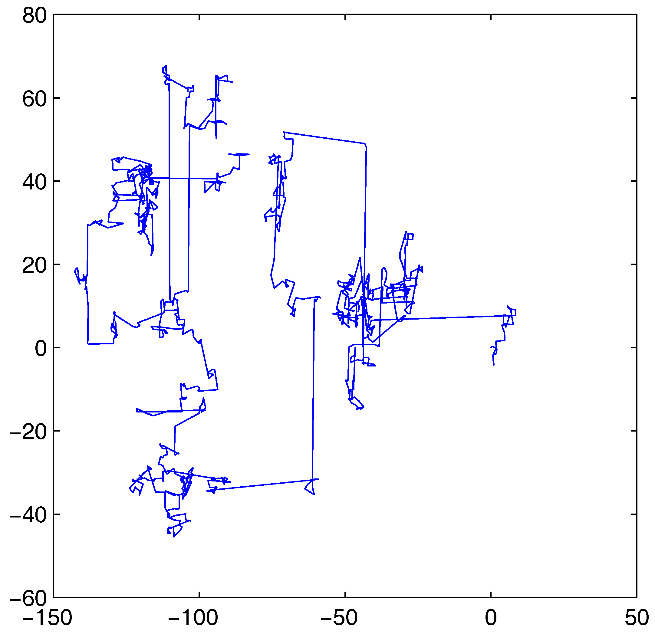
where s is the step-size with $1<\lambda \le 3$. Lévy flight can generate smaller step-size with high frequency and generate larger step-size occasionally. In the search process, the bee with a large step-size can reach anywhere of the entire search space to locate the potential optimal solution; when the bees are trapped in the local optimum, the large step-size can make the bees escape from the local optimum. The bees with a small step-size tend to fine-tune the current solution to obtain the optimal solution. The foraging behaviors of many creatures in nature satisfy Lévy flight, such as albatrosses’ foraging flight trajectory [27,28] and drosophilas’ intermittent foraging flight trajectory [29]. Viswanathan et al. suggest that Lévy flight is an optimal search strategy when the target sites are sparse and distributed randomly [26].

This paper uses the method proposed by [30] to calculate Lévy flight step-size:

$$s=\frac{u}{{\left|v\right|}^{1/\beta }}$$

(5)

where $\beta \in [0.3,1.99]$, u and v are two normal stochastic variables with standard deviation ${\sigma }_u$ and ${\sigma }_v$.

$$u\sim N(0,{\sigma }_u^2),v\sim N(0,{\sigma }_v^2)$$

(6)

$${\sigma }_u={\left\{\frac{\mathsf{\Gamma }(1+\beta )sin(\pi \beta /2)}{\mathsf{\Gamma }[(1+\beta )/2]2^{(\beta -1)/2}\beta }\right\}}^{1/\beta },{\sigma }_v=1$$

(7)

where the notation $\mathsf{\Gamma }(z)$ is gamma function. If the real part of the complex number z is positive $(Re(z)>0)$, then the integral

$$\mathsf{\Gamma }(z)={\int }_0^{\infty }{x}^{z-1}{e}^{-x}dx$$

(8)

converges absolutely.

As shown in Figure 1, Lévy flight with a mix of large step-size and small step-size can balance exploration and exploitation. Therefore, SLABC introduces Lévy flight step-size to the modified SSEs to improve the performance.

3.2. The Modified Solution Search Equations

To solve the optimization problem, the intelligent optimization algorithm should combine global search methods with local search methods to balance exploration and exploitation. However, exploration strategies and exploitation strategies contradict each other and one SSE in ABC algorithm cannot balance two aspects. Therefore, this paper proposes an achievable ABC algorithm which uses five SSEs as the candidate operator pool.

Following the classical ABC algorithm, SLABC employs the original SSE as the first search equations to improve exploration of SLABC algorithm.

$$v_{i,j}=x_{i,j}+c_1(x_{i,j}-x_{r1,j})$$

(9)

where $r1\in \{1,2,\dots ,SN\}$ and $j\in \{1,2,\dots ,D\}$ are randomly chosen indexes; $r1$ is different with i; $c_1$ is a random number in the range $[-1.0,1.0]$.

To improve exploitation, the second SSE introduces the global best solution to guide the new candidate solutions towards the global best solution.

$$v_{i,j}=x_{i,j}+c_2(x_{gbest}-x_{i,j})$$

(10)

where $x_{gbest}$ is the global best solution. Generally speaking, there may be a better solution around the global best solution; therefore, we set random number $c_2$ in the range $[0.75,1.25]$.

The Equation (9) is good at exploration and Equation (10) is good at exploitation, therefore to well balance exploration and exploitation, the third SSE combine the two equations as follows.

$$v_{i,j}=x_{i,j}+c_3(x_{i,j}-x_{r2,j})+c_4(x_{gbest}-x_{i,j})$$

(11)

where $r2\in \{1,2,\dots ,SN\}$ are randomly chosen indexes and $r2$ is different with i; $c_3\in [-0.5,0.5]$ and $c_4\in [0.5,1.5]$ are random numbers.

It seems that the global optimal solution is most likely around the best solution of the previous iteration. Therefore, the fourth SSE is the same with the one proposed in MABC algorithm which is based on that the bee searches only around the best solution of the previous iteration to improve the exploitation.

$$v_{i,j}=x_{gbest}+c_5(x_{r3,j}-x_{r4,j})$$

(12)

where $r3$ and $r4$ are mutually different random integer indices selected from $\{1,2,\dots ,SN\}$; $c_5$ is a random number in the range $[-0.5,0.5]$.

Because the above four SSEs are based on the current solutions, when the present solutions converge to the similar point or are trapped in local optimum, the above SSEs cannot escape from the local minimum effectively. Therefore, this paper introduces Lévy flight step-size to the last SSE to solve this problem.

$$v_{i,j}=x_{i,j}+s$$

(13)

where s is the Lévy flight step-size which can be calculated in Equation (5).

Different from the GABC, MABC algorithm, the range of the weight $c_3$, $c_4$, $c_5$ in Equations (11) and (12) with the $g_{best}$ term are all reduced and the interval length are set to 1. Therefore, the new generated candidate solution can be in a smaller range and the accuracy of the solution will be improved. Moreover, to make the candidate solution nearer to the global best solution, the range of the weight $c_2$ in Equation (10) is further reduced and interval length are set to 0.5.

After all the employed (onlooker) bees produce the new candidate solutions using the improved SSEs, then, a greedy selection mechanism is used to select a better solution between $x_i$ and $v_i$.

3.3. Self-Learning Mechanism

The five SSEs are regarded as the candidate operator pool and different operator is more effective at different stage. At each iteration, each employed (onlooker) bee will select a SSE from the candidate operator pool to update the corresponding solution. This paper proposes a simple self-learning mechanism to realize such optimal choice, wherein the SSE is selected according to the previous success ratio in generating promising solutions at each iteration.

In the self-learning mechanism, each SSE is assigned to a probability: success ratio. It is defined as

$$Sra{t}_k=\frac{S_k}{T_k},k=1,2,\dots ,5$$

(14)

where $S_k$ denotes the counter that records the number of successful updating times of the k-th SSE, where the new candidate solution is better than the old one; $T_k$ is the total number of updating times of the k-th SSE is selected; $Sra{t}_k$ is the success ratio of the k-th SSE. At each iteration, each SSE k is selected according to the success ratio $Sra{t}_k$ through roulette wheel selection. The new candidate solutions are then produced by the selected SSE. In the initialization stage, each success ratio $Srat{e}_k$ is given an equal selection probability.

It is well known that at the early stage of the optimization, the bees are inclined to locate the potential optimal regions by wandering through the entire search space. Conversely, most of the bees are apt to fine-tune the present solutions to obtain the global optimal solution at the latter stage of the optimization. Therefore, in order to avoid the interference between the early stage and the latter stage, this paper divides the whole optimization process into two stages. At each stage, $S_k$, $T_k$ and the success ratio $Srat{e}_k$ all will be initialized.

3.4. Description of the SLABC Algorithm

The pseudo code of the SLABC algorithm can be described as follows (Algorithm 1):

Algorithm 1

Initialize the population of the bees as N and $SN=N/2$; set the number of trials as $limit$.

Randomly generate $SN$ points $x_i(i=1,2,\dots ,SN)$ in the search space to form an initial solution.

Find the global best solution $gbest$ and the its position $x_{gbest}$ from the $SN$ points.

Set the maximum number of function evaluations, $Max.FE$; $S_k=1$, $T_k=1$ and $Srat{e}_k=0.2$.

While$FE<Max.FE$

If$FE=1+Max.FE/2$

Initialize $S_k$, $T_k$ and $Srat{e}_k$.

End If

Employed bee stage:

for$i=1$ to $SN$

Set the candidate solution $v_i=x_i$ and randomly choose j from $\{1,2,\dots ,D\}$.

Randomly choose a SSE k from the candidate strategy pool through roulette wheel selection

and count $T_k=T_k+1$.

Update the candidate solution $v_i$ using the selected SSE.

If $f(v_i)<f(x_i)$

$x_i=v_i$, $S_k=S_k+1$, $trial(i)=1$.

Else

$trial(i)=trial(i)+1$.

End If

End For

Update the $gbest$ and $x_{gbest}$ and calculate the probability value $P_i$ using Equation (2).

Onlooker bee stage:

for$i=1$ to $SN$

Select one solution to update based on $P_i$ and roulette wheel selection.

The update process is same as that in the employed bee stage.

End For

Update the $gbest$ and $x_{gbest}$ and calculate the probability value $P_i$ using Equation (2).

Scout stage:

If $trial(i)>limit$

Initialize $x_i$ with a new randomly generated point in the search space.

End If

$FE=FE+1$

End While

4. Experiments and Results

4.1. Experimental Setup

To investigate the performance of the SLABC algorithm, 9 benchmark functions shown in

Table 1. Numerical benchmark functions.

Type	Test Function	Formulation	Search Range	Minimum Value
Unimodal	Sphere	$f_1(\overrightarrow{x})={\displaystyle \sum _{i=1}^D}{x}_i^2$	$x_i\in [-100,100]$	$f_1(\overrightarrow{0})=0$
	Quartic	$f_2(\overrightarrow{x})={\displaystyle \sum _{i=1}^D}{ix}_i^4+random[0,1)$	$x_i\in [-1.28,1.28]$	$f_2(\overrightarrow{0})=0$
	Schwefel’s Problem 2.22	$f_3(\overrightarrow{x})={\displaystyle \sum _{i=1}^D}\left|x_i\right|+{\displaystyle \prod _{i=1}^D}\left|x_i\right|$	$x_i\in [-10,10]$	$f_3(\overrightarrow{0})=0$
	Rosenbrock	$f_4(\overrightarrow{x})={\displaystyle \sum _{i=1}^{D-1}}[100(x_{i+1}-x_i{)}^2+(1-x_i{)}^2]$	$x_i\in [-30,30]$	$f_4(\overrightarrow{1})=0$
Multimodal	Rastrigin	$f_5(\overrightarrow{x})={\displaystyle \sum _{i=1}^D}{[x}_i^2-10cos(2\pi x_i)+10]$	$x_i\in [-5.12,5.12]$	$f_5(\overrightarrow{0})=0$
	Griewank	$f_6(\overrightarrow{x})=\frac{1}{4000}{\displaystyle \sum _{i=1}^D}{x}_i^2-{\displaystyle \prod _{i=1}^D}cos(\frac{x_i}{\sqrt{i}})+1$	$x_i\in [-600,600]$	$f_6(\overrightarrow{0})=0$
	Ackley	$f_7(\overrightarrow{x})=-20exp(-0.2\sqrt{{\displaystyle \sum _{i=1}^D}{x}_i^2/D})+20-exp({\displaystyle \sum _{i=1}^D}cos(2\pi x_i)/D)+e$	$x_i\in [-30,30]$	$f_7(\overrightarrow{0})=0$
	Schwefel’s Problem 2.26	$f_8(\overrightarrow{x})=418.9829D-{\displaystyle \sum _{i=1}^D}(x_{i}sin(\sqrt{\left|x_i\right|}))$	$x_i\in [-500,500]$	$f_8(\overrightarrow{420.9687})=0$
	Penalized	$f_9(\overrightarrow{x})=0.1\left\{{sin}^2(3\pi x_1)+{\displaystyle \sum _{i=1}^{D-1}}{(x_i-1)}^2[1+{sin}^2(3\pi x_{i+1})]+{(x_D-1)}^2\right\}$	$x_i\in [-50,50]$	$f_9(\overrightarrow{1})=0$
		+${\displaystyle \sum _{i=1}^D}u(x_i,5,100,4)$

were used, including four unimodal functions ($f_1-f_4$) and five multimodal functions ($f_5-f_9$). In Table 1, D denotes the dimensions of the solution space and 30, 60, and 100 dimensions are used in the present paper. The unimodal functions can be used to analyse the convergence rate of the algorithms. The multimodal functions are commonly used to show whether the algorithms can escape from the local optimum effectively.

The effectiveness of the proposed SLABC algorithm was evaluated by comparing its results with other related algorithms, such as ABC [2], GABC [20], MABC [21], and distABC [24]. To make a fair comparison among ABCs, all the algorithms were tested using the same parameters: the population size $N=100$, $limit=100$, the maximum number of iterations, $Max.FE=2000$. Additionally, other specific parameters of each comparison algorithm are same as in ABC [2], GABC [20], MABC [21], and distABC [24]. In order to ensure the experiment results stability, we repeated each algorithm for 20 times and average the results.

4.2. Experimental Results

This paper uses five indexes to analysis the experimental results: the best solution (Best), median solution (Median), worst solution (Worst), average solution (Mean), and standard deviation (Std).

Table 2. Comparison between SLABC and other algorithms for 20 times independent runs tested on 9 basic benchmark functions with 30 dimensions.

Functions	Metrics	ABC	MABC	GABC	distABC	SLABC
	Best	3.68 × 10${}^{-26}$	2.53 × 10${}^{-38}$	9.03 × 10${}^{-46}$	4.21 × 10${}^{-42}$	3.49 × 10${}^{-65}$
	Median	1.55 × 10${}^{-25}$	2.96 × 10${}^{-20}$	3.83 × 10${}^{-45}$	3.06 × 10${}^{-40}$	3.32 × 10${}^{-64}$
$f_1$	Worst	2.91 × 10${}^{-24}$	2.23 × 10${}^{-1}$	1.89 × 10${}^{-44}$	1.82 × 10${}^{-37}$	1.25 × 10${}^{-62}$
	Mean	4.25 × 10${}^{-25}$	1.12 × 10${}^{-2}$	6.50 × 10${}^{-45}$	9.71 × 10${}^{-39}$	1.33 × 10${}^{-63}$
	Std	6.73 × 10${}^{-24}$	4.99 × 10${}^{-2}$	5.98 × 10${}^{-45}$	4.06 × 10${}^{-38}$	2.83 × 10${}^{-63}$
	Best	2.18 × 10${}^{-64}$	7.26 × 10${}^{-81}$	8.34 × 10${}^{-99}$	3.47 × 10${}^{-88}$	6.50 × 10${}^{-133}$
	Median	6.66 × 10${}^{-63}$	9.75 × 10${}^{-53}$	3.13 × 10${}^{-97}$	1.70 × 10${}^{-85}$	3.47 × 10${}^{-130}$
$f_2$	Worst	4.85 × 10${}^{-61}$	1.21 × 10${}^{-9}$	9.61 × 10${}^{-96}$	7.77 × 10${}^{-80}$	6.18 × 10${}^{-128}$
	Mean	3.86 × 10${}^{-62}$	6.06 × 10${}^{-11}$	1.35 × 10${}^{-96}$	4.24 × 10${}^{-81}$	5.81 × 10${}^{-129}$
	Std	1.06 × 10${}^{-61}$	2.71 × 10${}^{-10}$	2.42 × 10${}^{-96}$	1.73 × 10${}^{-80}$	1.51 × 10${}^{-128}$
	Best	4.66 × 10${}^{-15}$	1.32 × 10${}^{-20}$	1.75 × 10${}^{-24}$	1.13 × 10${}^{-21}$	2.89 × 10${}^{-35}$
	Median	8.28 × 10${}^{-15}$	2.70 × 10${}^{-20}$	4.49 × 10${}^{-24}$	4.02 × 10${}^{-21}$	7.69 × 10${}^{35}$
$f_3$	Worst	1.46 × 10${}^{-14}$	5.83 × 10${}^{-6}$	8.59 × 10${}^{-24}$	7.47 × 10${}^{-18}$	2.50 × 10${}^{-34}$
	Mean	8.86 × 10${}^{-15}$	2.92 × 10${}^{-7}$	4.52 × 10${}^{-24}$	4.75 × 10${}^{-19}$	8.31 × 10${}^{-35}$
	Std	3.05 × 10${}^{-15}$	1.30 × 10${}^{-6}$	1.44 × 10${}^{-24}$	1.70 × 10${}^{-18}$	5.02 × 10${}^{-35}$
	Best	4.79 × 10${}^{-3}$	6.89 × 10${}^{-2}$	1.19 × 10${}^{-3}$	8.89 × 10${}^{-3}$	1.50 × 10${}^{-4}$
	Median	9.91 × 10${}^{-2}$	2.54× 10${}^0$	9.07 × 10${}^{-2}$	6.26 × 10${}^{-2}$	1.09 × 10${}^{-1}$
$f_4$	Worst	1.01 × 10${}^0$	1.59 × 10${}^2$	2.40 × 10${}^0$	2.98 × 10${}^{-1}$	7.54 × 10${}^1$
	Mean	1.34 × 10${}^{-1}$	2.16 × 10${}^0$	3.32 × 10${}^{-1}$	8.84 × 10${}^{-2}$	9.87 × 10${}^0$
	Std	2.10 × 10${}^{-1}$	4.19 × 10${}^1$	5.44 × 10${}^{-1}$	8.88 × 10${}^{-2}$	2.24 × 10${}^1$
	Best	0.00 × 10${}^0$	0.00 × 10${}^0$	0.00 × 10${}^0$	0.00 × 10${}^0$	0.00 × 10${}^0$
	Median	0.00 × 10${}^0$	6.21 × 10${}^{-13}$	0.00 × 10${}^0$	0.00 × 10${}^0$	0.00 × 10${}^0$
$f_5$	Worst	3.55 × 10${}^{-15}$	1.15 × 10${}^{-1}$	0.00 × 10${}^0$	0.00 × 10${}^0$	0.00 × 10${}^0$
	Mean	5.33 × 10${}^{-16}$	9.82 × 10${}^{-3}$	0.00 × 10${}^0$	0.00 × 10${}^0$	0.00 × 10${}^0$
	Std	1.01 × 10${}^{-15}$	2.87 × 10${}^{-2}$	0.00 × 10${}^0$	0.00 × 10${}^0$	0.00 × 10${}^0$
	Best	0.00 × 10${}^0$	0.00 × 10${}^0$	0.00 × 10${}^0$	0.00 × 10${}^0$	0.00 × 10${}^0$
	Median	3.00 × 10${}^{-15}$	1.94 × 10${}^{-15}$	0.00 × 10${}^0$	0.00 × 10${}^0$	0.00 × 10${}^0$
$f_6$	Worst	3.08 × 10${}^{-8}$	5.47 × 10${}^{-1}$	1.55 × 10${}^{-15}$	0.00 × 10${}^0$	0.00 × 10${}^0$
	Mean	1.54 × 10${}^{-9}$	5.47 × 10${}^{-2}$	1.67 × 10${}^{-16}$	0.00 × 10${}^0$	0.00 × 10${}^0$
	Std	6.88 × 10${}^{-9}$	1.58 × 10${}^{-1}$	4.00 × 10${}^{-16}$	0.00 × 10${}^0$	0.00 × 10${}^0$
	Best	1.21 × 10${}^{-13}$	2.13 × 10${}^{-14}$	3.20 × 10${}^{-14}$	3.20 × 10${}^{-14}$	2.49 × 10${}^{-14}$
	Median	2.13 × 10${}^{-13}$	2.96 × 10${}^{-12}$	3.73 × 10${}^{-14}$	3.91 × 10${}^{-14}$	2.84 × 10${}^{-14}$
$f_7$	Worst	3.66 × 10${}^{-13}$	3.29 × 10${}^{-1}$	4.26 × 10${}^{-14}$	3.91 × 10${}^{-14}$	3.20 × 10${}^{-14}$
	Mean	2.15 × 10${}^{-13}$	1.70 × 10${}^{-2}$	3.66 × 10${}^{-14}$	3.59 × 10${}^{-14}$	2.81 × 10${}^{-14}$
	Std	6.17 × 10${}^{-14}$	7.34 × 10${}^{-2}$	3.66 × 10${}^{-15}$	3.63 × 10${}^{-15}$	1.96 × 10${}^{-15}$
	Best	3.82 × 10${}^{-4}$	3.82 × 10${}^{-4}$	3.82 × 10${}^{-4}$	3.82 × 10${}^{-4}$	3.82 × 10${}^{-4}$
	Median	3.82 × 10${}^{-4}$	3.82 × 10${}^{-4}$	3.82 × 10${}^{-4}$	3.82 × 10${}^{-4}$	3.82 × 10${}^{-4}$
$f_8$	Worst	2.62 × 10${}^{-3}$	1.38 × 10${}^0$	3.82 × 10${}^{-4}$	3.82 × 10${}^{-4}$	3.82 × 10${}^{-4}$
	Mean	4.94 × 10${}^{-4}$	9.12 × 10${}^{-2}$	3.82 × 10${}^{-4}$	3.82 × 10${}^{-4}$	3.82 × 10${}^{-4}$
	Std	5.00 × 10${}^{-4}$	3.17 × 10${}^{-1}$	2.83 × 10${}^{-10}$	1.44 × 10${}^{-11}$	7.46 × 10${}^{-13}$
	Best	1.29 × 10${}^{-26}$	1.35 × 10${}^{-32}$	1.35 × 10${}^{-32}$	4.47 × 10${}^{-21}$	1.35 × 10${}^{-32}$
	Median	1.20 × 10${}^{-25}$	5.23 × 10${}^{-15}$	1.35 × 10${}^{-32}$	2.83 × 10${}^{-20}$	1.35 × 10${}^{-32}$
$f_9$	Worst	9.62 × 10${}^{-25}$	2.46 × 10${}^{-2}$	1.35 × 10${}^{-32}$	9.43 × 10${}^{-20}$	1.35 × 10${}^{-32}$
	Mean	2.20 × 10${}^{-25}$	2.67 × 10${}^{-3}$	1.35 × 10${}^{-32}$	3.38 × 10${}^{-20}$	1.35 × 10${}^{-32}$
	Std	2.51 × 10${}^{-25}$	6.79 × 10${}^{-3}$	2.81 × 10${}^{-48}$	2.68 × 10${}^{-20}$	2.81 × 10${}^{-48}$

,

Table 3. Comparison between SLABC and other algorithms for 20 times independent runs tested on 9 basic benchmark functions with 60 dimensions.

Functions	Metrics	ABC	MABC	GABC	distABC	SLABC
	Best	2.39 × 10${}^{-10}$	4.34 × 10${}^{-15}$	1.37 × 10${}^{-19}$	2.21 × 10${}^{-18}$	1.99 × 10${}^{-29}$
	Median	1.85 × 10${}^{-9}$	3.52 × 10${}^{-5}$	7.20 × 10${}^{-19}$	9.82 × 10${}^{-18}$	8.70 × 10${}^{-29}$
$f_1$	Worst	1.50 × 10${}^{-8}$	2.36 × 10${}^1$	3.13 × 10${}^{-18}$	4.51 × 10${}^{-17}$	4.59 × 10${}^{-28}$
	Mean	3.40 × 10${}^{-9}$	2.32 × 10${}^0$	9.29 × 10${}^{-19}$	1.46 × 10${}^{-17}$	1.25 × 10${}^{-28}$
	Std	4.09 × 10${}^{-8}$	6.64 × 10${}^0$	7.59 × 10${}^{-19}$	1.26 × 10${}^{-17}$	1.06 × 10${}^{-28}$
	Best	1.52 × 10${}^{-28}$	6.94 × 10${}^{-36}$	1.38 × 10${}^{-46}$	1.42 × 10${}^{-41}$	1.79 × 10${}^{-61}$
	Median	3.72 × 10${}^{-27}$	1.46 × 10${}^{-23}$	3.09 × 10${}^{-45}$	1.59 × 10${}^{-40}$	5.17 × 10${}^{-60}$
$f_2$	Worst	7.55 × 10${}^{-26}$	1.22 × 10${}^{-6}$	2.74 × 10${}^{-44}$	2.23 × 10${}^{-39}$	2.17 × 10${}^{-58}$
	Mean	1.20 × 10${}^{-26}$	7.83 × 10${}^{-8}$	6.22 × 10${}^{-45}$	2.85 × 10${}^{-40}$	2.75 × 10${}^{-59}$
	Std	1.95 × 10${}^{-26}$	2.79 × 10${}^{-7}$	7.46 × 10${}^{-45}$	4.87 × 10${}^{-40}$	5.94 × 10${}^{-59}$
	Best	3.91 × 10${}^{-6}$	1.21 × 10${}^{-8}$	6.66 × 10${}^{-11}$	1.06 × 10${}^{-9}$	3.23 × 10${}^{-16}$
	Median	6.91 × 10${}^{-6}$	8.46 × 10${}^{-7}$	8.17 × 10${}^{-11}$	2.02 × 10${}^{-9}$	6.49 × 10${}^{-16}$
$f_3$	Worst	1.27 × 10${}^{-5}$	1.31 × 10${}^0$	1.65 × 10${}^{-10}$	4.96 × 10${}^{-9}$	1.24 × 10${}^{-15}$
	Mean	7.55 × 10${}^{-6}$	1.79 × 10${}^{-1}$	9.41 × 10${}^{-11}$	2.18 × 10${}^{-9}$	6.75 × 10${}^{-16}$
	Std	2.44 × 10${}^{-6}$	3.58 × 10${}^{-1}$	2.77 × 10${}^{-11}$	9.43 × 10${}^{-10}$	2.71 × 10${}^{-16}$
	Best	1.84 × 10${}^{-1}$	7.88 × 10${}^0$	1.97 × 10${}^{-2}$	1.15 × 10${}^{-1}$	4.53 × 10${}^{-2}$
	Median	2.25 × 10${}^0$	1.46 × 10${}^2$	3.26 × 10${}^{-1}$	8.01 × 10${}^{-1}$	2.48 × 10${}^0$
$f_4$	Worst	8.50 × 10${}^0$	7.63 × 10${}^2$	8.43 × 10${}^1$	2.17 × 10${}^0$	8.20 × 10${}^1$
	Mean	2.74 × 10${}^0$	2.32 × 10${}^2$	1.03 × 10${}^1$	8.82 × 10${}^{-1}$	1.07 × 10${}^{-1}$
	Std	2.41 × 10${}^0$	2.24 × 10${}^2$	2.45 × 10${}^1$	5.49 × 10${}^{-1}$	2.43 × 10${}^{-1}$
	Best	2.59 × 10${}^{-9}$	2.52 × 10${}^{-13}$	3.55 × 10${}^{-15}$	1.21 × 10${}^{-11}$	0.00 × 10${}^0$
	Median	9.13 × 10${}^{-2}$	1.87 × 10${}^{-9}$	4.35 × 10${}^{-14}$	6.74 × 10${}^{-5}$	0.00 × 10${}^0$
$f_5$	Worst	1.99 × 10${}^0$	1.46 × 10${}^1$	1.03 × 10${}^{-12}$	9.95 × 10${}^{-1}$	0.00 × 10${}^0$
	Mean	4.89 × 10${}^{-1}$	9.33 × 10${}^{-1}$	1.79 × 10${}^{-13}$	1.09 × 10${}^{-1}$	0.00 × 10${}^0$
	Std	5.92 × 10${}^{-1}$	3.33 × 10${}^0$	2.92 × 10${}^{-13}$	3.04 × 10${}^{-1}$	0.00 × 10${}^0$
	Best	2.04 × 10${}^{-10}$	8.48 × 10${}^{-14}$	0.00 × 10${}^0$	0.00 × 10${}^{-0}$	0.00 × 10${}^0$
	Median	1.51 × 10${}^{-9}$	9.96 × 10${}^{-5}$	2.78 × 10${}^{-16}$	1.67 × 10${}^{-16}$	0.00 × 10${}^0$
$f_6$	Worst	1.50 × 10${}^{-8}$	1.31 × 10${}^0$	4.86 × 10${}^{-10}$	6.00 × 10${}^{-15}$	6.66 × 10${}^{-16}$
	Mean	3.98 × 10${}^{-9}$	3.71 × 10${}^{-1}$	2.64 × 10${}^{-11}$	7.94 × 10${}^{-16}$	5.55 × 10${}^{-17}$
	Std	4.92 × 10${}^{-9}$	5.00 × 10${}^{-1}$	1.08 × 10${}^{-10}$	1.48 × 10${}^{-15}$	1.75 × 10${}^{-16}$
	Best	6.89 × 10${}^{-6}$	1.14 × 10${}^{-7}$	3.31 × 10${}^{-10}$	7.60 × 10${}^{-9}$	3.73 × 10${}^{-3}$
	Median	1.50 × 10${}^{-5}$	6.23 × 10${}^{-4}$	5.25 × 10${}^{-10}$	1.04 × 10${}^{-8}$	5.17 × 10${}^{-13}$
$f_7$	Worst	6.14 × 10${}^{-5}$	1.26 × 10${}^0$	6.87 × 10${}^{-10}$	1.44e × 10${}^{-8}$	6.43 × 10${}^{-13}$
	Mean	1.72 × 10${}^{-5}$	1.31 × 10${}^{-1}$	5.11 × 10${}^{-10}$	1.07 × 10${}^{-8}$	5.08 × 10${}^{-13}$
	Std	1.16 × 10${}^{-5}$	3.21 × 10${}^{-1}$	9.52 × 10${}^{-11}$	2.16 × 10${}^{-9}$	7.29 × 10${}^{-14}$
	Best	3.57 × 10${}^2$	7.64 × 10${}^{-4}$	7.64 × 10${}^{-4}$	2.41 × 10${}^2$	7.64 × 10${}^{-4}$
	Median	6.26 × 10${}^2$	7.64 × 10${}^4$	2.84 × 10${}^3$	5.61 × 10${}^2$	7.64 × 10${}^{-4}$
$f_8$	Worst	9.50 × 10${}^2$	9.39 × 10${}^1$	3.61 × 10${}^2$	7.22 × 10${}^2$	7.64 × 10${}^{-4}$
	Mean	6.75 × 10${}^2$	5.13 × 10${}^0$	4.86 × 10${}^1$	5.20 × 10${}^2$	7.64 × 10${}^{-4}$
	Std	2.01 × 10${}^2$	2.10 × 10${}^1$	9.68 × 10${}^1$	1.31 × 10${}^2$	1.43 × 10${}^{-9}$
	Best	9.97 × 10${}^{-10}$	5.76 × 10${}^{-16}$	9.00 × 10${}^{-20}$	9.85 × 10${}^{-12}$	2.44e × 10${}^{-30}$
	Median	4.95 × 10${}^{-9}$	1.70 × 10${}^{-4}$	3.15 × 10${}^{-19}$	4.72 × 10${}^{-11}$	2.89 × 10${}^{-29}$
$f_9$	Worst	1.30 × 10${}^{-8}$	4.76 × 10${}^0$	1.76 × 10${}^{-18}$	9.28 × 10${}^{-11}$	1.12 × 10${}^{-28}$
	Mean	5.43 × 10${}^{-9}$	3.70 × 10${}^{-1}$	4.55 × 10${}^{-19}$	4.45 × 10${}^{-11}$	3.45 × 10${}^{-29}$
	Std	3.24 × 10${}^{-9}$	1.08 × 10${}^0$	4.09e × 10${}^{-19}$	1.83 × 10${}^{-11}$	2.84 × 10${}^{-29}$

and

Table 4. Comparison between SLABC and other algorithms for 20 times independent runs tested on 9 basic benchmark functions with 100 dimensions.

Functions	Metrics	ABC	MABC	GABC	distABC	SLABC
	Best	1.11 × 10${}^{-6}$	3.72 × 10${}^{-6}$	3.28 × 10${}^{-10}$	2.29 × 10${}^{-10}$	5.23 × 10${}^{-16}$
	Median	7.55 × 10${}^{-6}$	3.45 × 10${}^{-1}$	2.25 × 10${}^{-9}$	2.10 × 10${}^{-9}$	1.79 × 10${}^{-15}$
$f_1$	Worst	4.46 × 10${}^{-5}$	1.12 × 10${}^2$	4.01 × 10${}^{-9}$	2.71 × 10${}^{-7}$	7.16 × 10${}^{-15}$
	Mean	1.25 × 10${}^{-5}$	1.82 × 10${}^1$	2.11 × 10${}^{-9}$	1.82 × 10${}^{-8}$	2.46 × 10${}^{-15}$
	Std	1.27 × 10${}^{-5}$	3.55 × 10${}^1$	1.02 × 10${}^{-9}$	6.00 × 10${}^{-8}$	1.87 × 10${}^{-15}$
	Best	7.38 × 10${}^{-17}$	3.76 × 10${}^{-18}$	1.21 × 10${}^{-25}$	1.67 × 10${}^{-23}$	4.98 × 10${}^{-35}$
	Median	9.25 × 10${}^{-16}$	9.42 × 10${}^{-12}$	4.18 × 10${}^{-25}$	1.16 × 10${}^{-21}$	3.08 × 10${}^{-34}$
$f_2$	Worst	1.84 × 10${}^{-14}$	1.48 × 10${}^{-3}$	2.23 × 10${}^{-24}$	5.76 × 10${}^{-21}$	2.10 × 10${}^{-32}$
	Mean	3.04 × 10${}^{-15}$	1.38 × 10${}^{-4}$	5.64 × 10${}^{-25}$	1.73 × 10${}^{-21}$	2.68 × 10${}^{-33}$
	Std	4.56 × 10${}^{-15}$	3.61 × 10${}^{-4}$	4.75 × 10${}^{-25}$	1.71 × 10${}^{-21}$	5.43 × 10${}^{-33}$
	Best	1.79 × 10${}^{-3}$	7.51 × 10${}^{-4}$	6.21 × 10${}^{-6}$	7.15 × 10${}^{-5}$	3.87 × 10${}^{-9}$
	Median	2.71 × 10${}^{-3}$	2.28 × 10${}^{-2}$	1.39 × 10${}^{-5}$	1.35 × 10${}^{-4}$	9.02 × 10${}^{-9}$
$f_3$	Worst	5.86 × 10${}^{-3}$	8.83 × 10${}^0$	3.36 × 10${}^{-5}$	1.70 × 10${}^{-4}$	2.08 × 10${}^{-8}$
	Mean	3.11 × 10${}^{-3}$	8.79 × 10${}^{-1}$	1.57 × 10${}^{-5}$	1.30 × 10${}^{-4}$	9.2 × 10${}^{-9}$
	Std	1.26 × 10${}^{-3}$	2.25 × 10${}^0$	6.59 × 10${}^{-6}$	2.92 × 10${}^{-5}$	3.57 × 10${}^{-9}$
	Best	9.12 × 10${}^0$	1.46 × 10${}^2$	2.95 × 10${}^{-1}$	3.48 × 10${}^0$	2.66 × 10${}^{-2}$
	Median	2.68 × 10${}^1$	1.17 × 10${}^3$	8.00 × 10${}^1$	1.71 × 10${}^1$	3.60 × 10${}^0$
$f_4$	Worst	8.31 × 10${}^1$	1.14 × 10${}^4$	1.88 × 10${}^2$	4.78 × 10${}^1$	1.45 × 10${}^2$
	Mean	3.09 × 10${}^1$	2.28 × 10${}^3$	6.83 × 10${}^1$	1.87 × 10${}^1$	2.23 × 10${}^1$
	Std	1.83 × 10${}^1$	2.88 × 10${}^3$	5.76 × 10${}^1$	1.11 × 10${}^1$	3.98 × 10${}^1$
	Best	1.14 × 10${}^1$	1.47 × 10${}^{-4}$	1.08 × 10${}^0$	8.46 × 10${}^0$	1.11 × 10${}^{-10}$
	Median	1.70 × 10${}^1$	7.63 × 10${}^{-1}$	2.24 × 10${}^0$	1.08 × 10${}^1$	1.68 × 10${}^{-9}$
$f_5$	Worst	2.24 × 10${}^1$	6.76 × 10${}^1$	4.04 × 10${}^0$	1.30 × 10${}^1$	2.98 × 10${}^{-8}$
	Mean	1.67 × 10${}^1$	1.33 × 10${}^1$	2.55 × 10${}^0$	1.08 × 10${}^1$	4.55 × 10${}^{-9}$
	Std	3.17 × 10${}^0$	2.12 × 10${}^1$	8.29 × 10${}^{-1}$	1.23 × 10${}^0$	7.09 × 10${}^{-9}$
	Best	2.46 × 10${}^{-6}$	2.00 × 10${}^{-6}$	4.27 × 10${}^{-10}$	3.10 × 10${}^{-8}$	1.77 × 10${}^{-13}$
	Median	2.45 × 10${}^{-5}$	4.55 × 10${}^{-2}$	2.05 × 10${}^{-9}$	1.49 × 10${}^{-7}$	1.49 × 10${}^{-12}$
$f_6$	Worst	9.39 × 10${}^{-4}$	2.44 × 10${}^0$	6.47 × 10${}^{-7}$	2.27 × 10${}^{-6}$	1.18 × 10${}^{-11}$
	Mean	1.08 × 10${}^{-4}$	6.46 × 10${}^{-1}$	3.82 × 10${}^{-8}$	2.95 × 10${}^{-7}$	2.68 × 10${}^{-12}$
	Std	2.23 × 10${}^{-4}$	9.22 × 10${}^{-1}$	1.44 × 10${}^{-7}$	4.96 × 10${}^{-7}$	3.22 × 10${}^{-12}$
	Best	1.64 × 10${}^{-2}$	3.24 × 10${}^{-3}$	3.62 × 10${}^{-5}$	3.57 × 10${}^{-4}$	6.31 × 10${}^{-7}$
	Median	2.87 × 10${}^{-2}$	1.58 × 10${}^0$	5.56 × 10${}^{-5}$	5.75 × 10${}^{-4}$	1.09 × 10${}^{-6}$
$f_7$	Worst	4.93 × 10${}^{-2}$	4.17 × 10${}^{-0}$	8.04 × 10${}^{-5}$	1.26 × 10${}^{-3}$	1.56 × 10${}^{-6}$
	Mean	3.07 × 10${}^{-2}$	1.57 × 10${}^0$	5.65 × 10${}^{-5}$	6.24 × 10${}^{-4}$	1.12 × 10${}^{-6}$
	Std	1.03 × 10${}^{-2}$	1.42 × 10${}^0$	1.02 × 10${}^{-5}$	2.12 × 10${}^{-4}$	2.36 × 10${}^{-7}$
	Best	2.48 × 10${}^3$	2.55 × 10${}^{-3}$	8.72 × 10${}^2$	2.40 × 10${}^3$	1.27 × 10${}^{-3}$
	Median	3.25 × 10${}^3$	4.87 × 10${}^0$	1.44 × 10${}^3$	2.96 × 10${}^3$	1.27 × 10${}^{-3}$
$f_8$	Worst	3.63 × 10${}^3$	4.30 × 10${}^3$	1.77 × 10${}^3$	3.36 × 10${}^3$	1.18 × 10${}^2$
	Mean	3.13 × 10${}^3$	5.45 × 10${}^2$	1.36 × 10${}^3$	2.93 × 10${}^3$	1.21 × 10${}^1$
	Std	3.64 × 10${}^2$	9.98 × 10${}^2$	2.70 × 10${}^2$	2.36 × 10${}^2$	3.64 × 10${}^1$
	Best	3.64 × 10${}^{-6}$	9.56 × 10${}^{-7}$	4.88 × 10${}^{-10}$	9.79 × 10${}^{-9}$	8.47 × 10${}^{-17}$
	Median	3.25 × 10${}^{-5}$	8.28 × 10${}^{-1}$	2.26 × 10${}^{-9}$	5.90 × 10${}^{-8}$	3.34 × 10${}^{-16}$
$f_9$	Worst	4.98 × 10${}^{-4}$	4.75 × 10${}^0$	6.97 × 10${}^{-9}$	1.29 × 10${}^{-6}$	3.16 × 10${}^{-15}$
	Mean	5.95 × 10${}^{-5}$	1.15 × 10${}^0$	2.64 × 10${}^{-9}$	1.38 × 10${}^{-7}$	4.83 × 10${}^{-16}$
	Std	1.06 × 10${}^{-4}$	1.32 × 10${}^0$	1.57 × 10${}^{-9}$	2.85 × 10${}^{-7}$	6.58 × 10${}^{-16}$

show the experimental results obtained by each algorithm in the 20 independent runs. The results suggest that SLABC offers the higher solution accuracy on almost all the functions except function $f_4$ with $D=30,60,100$. It can be seen from the formulation of Rosenbrock function ($f_4$) that the first term $100{(x_{i+1}-x_i)}^2$ mainly influence the function value, which means that only the values among different dimensions in the candidate solutions are almost the same, the function value is smaller. Using the mean and standard deviation of the selected two solution, the distABC algorithm obtained the new candidate solutions, in which the values among different dimensions are of uniform size. Therefore, based on the distributed solution update rule, distABC algorithm gets the best results on Rosenbrock function ($f_4$).

Moreover, in the case of functions $f_5$, $f_6$, $f_8$ with $D=30$, the solution accuracy of SLABC are equal with the best of other algorithms. The Rastrigin function ($f_5$), Griewank function ($f_6$) and Schwefel’s Problem 2.26 function ($f_8$) are multimodal functions and are easy to obtain the optimal solutions with $D=30$. As the dimension gets higher, the difficulty of obtaining the optimal solution increases gradually. However, the solution accuracy of SLABC are better than the functions $f_5$, $f_6$, $f_8$ with $D=60$ and $D=100$, which proves that SLABC algorithm outperforms the other algorithms.

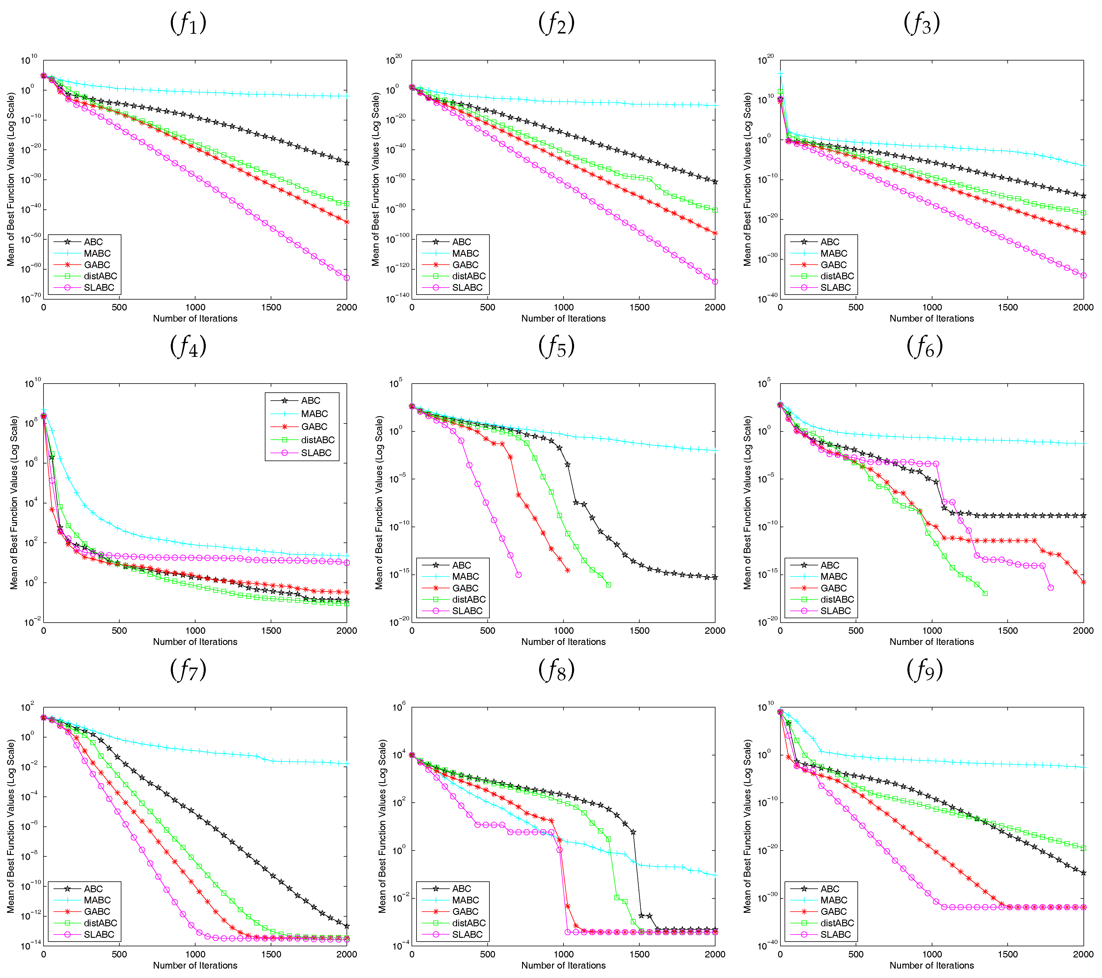
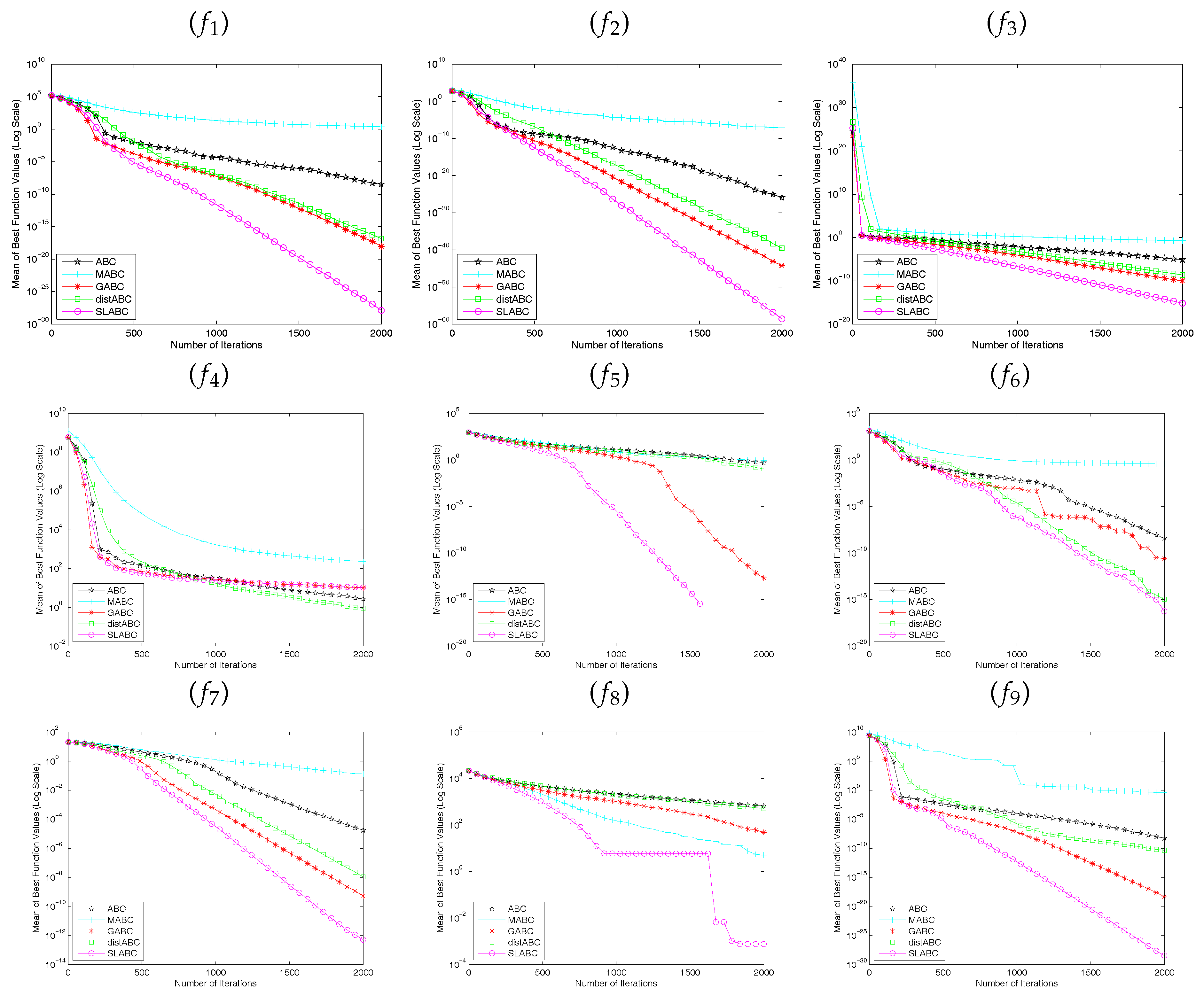
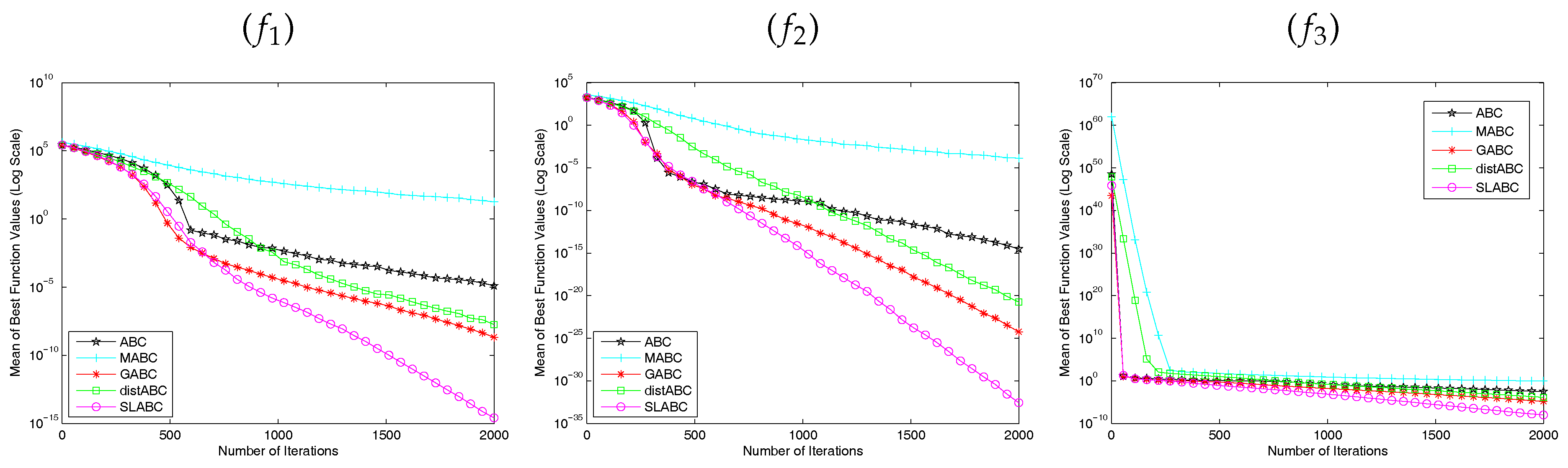
Figure 2, Figure 3 and Figure 4 show how the mean of the best solution for each algorithm changes with the number of iterations times. The lines that do not extend to the end of the experiments indicate that they have converged to 0 in the next calibration. As can be seen in the Figure 2, Figure 3 and Figure 4, the convergence rate of SLABC is faster than other algorithms except function $f_4$ with $D=30,60,100$ and function $f_6$ with $D=30$. The distABC algorithm is better than SLABC algorithm on the convergence rate and the accuracy of the solution. Though functions $f_5$, $f_6$, $f_8$ with $D=30$ get the same solution, SLABC algorithm converges faster than other algorithm on $f_5$, $f_8$ with $D=30$ and SLABC algorithm converges slower than distABC algorithm on $f_6$ with $D=30$. According to the above analysis, it is obvious that the performance of SLABC is more superior to other algorithms except distABC algorithm on Rosenbrock function ($f_4$).

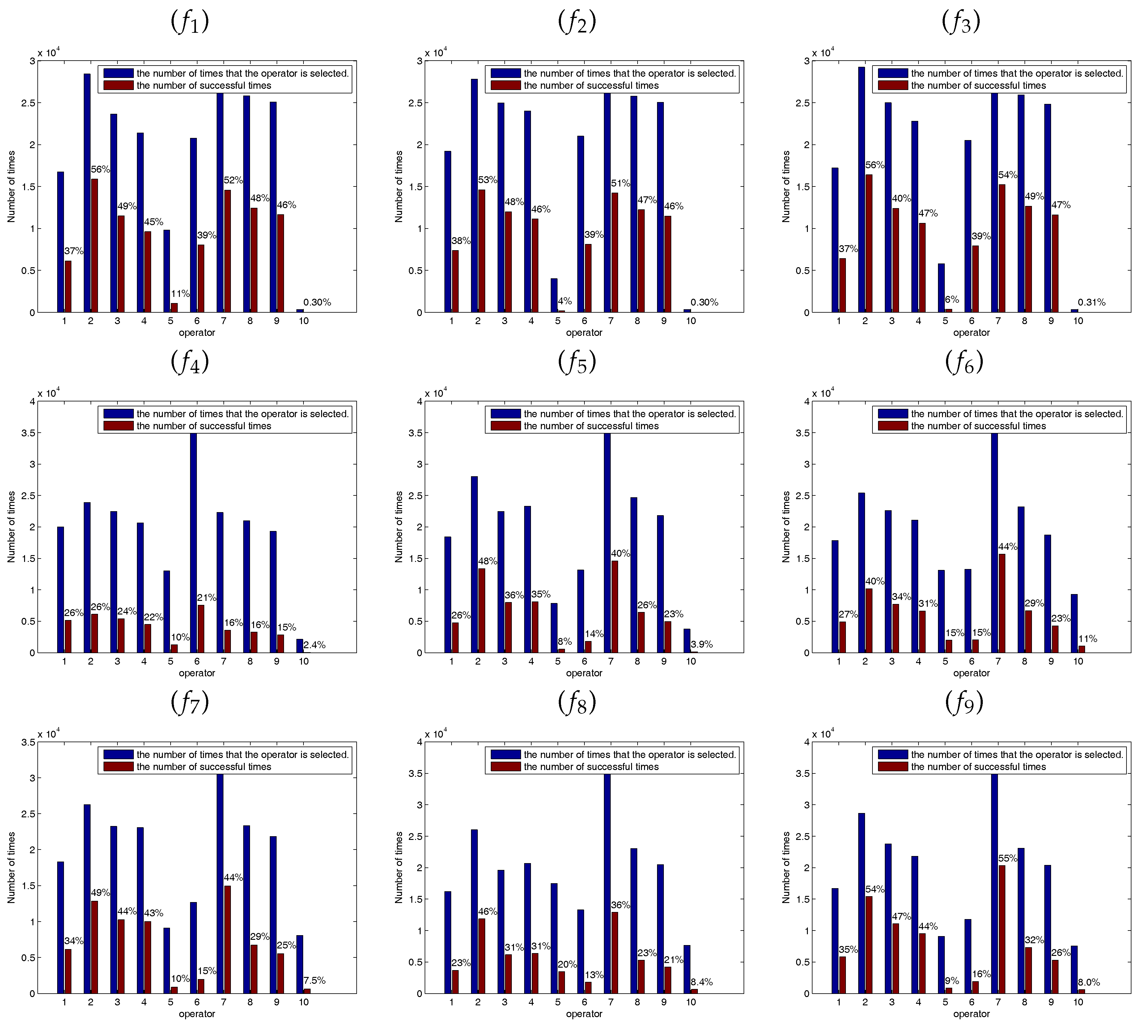
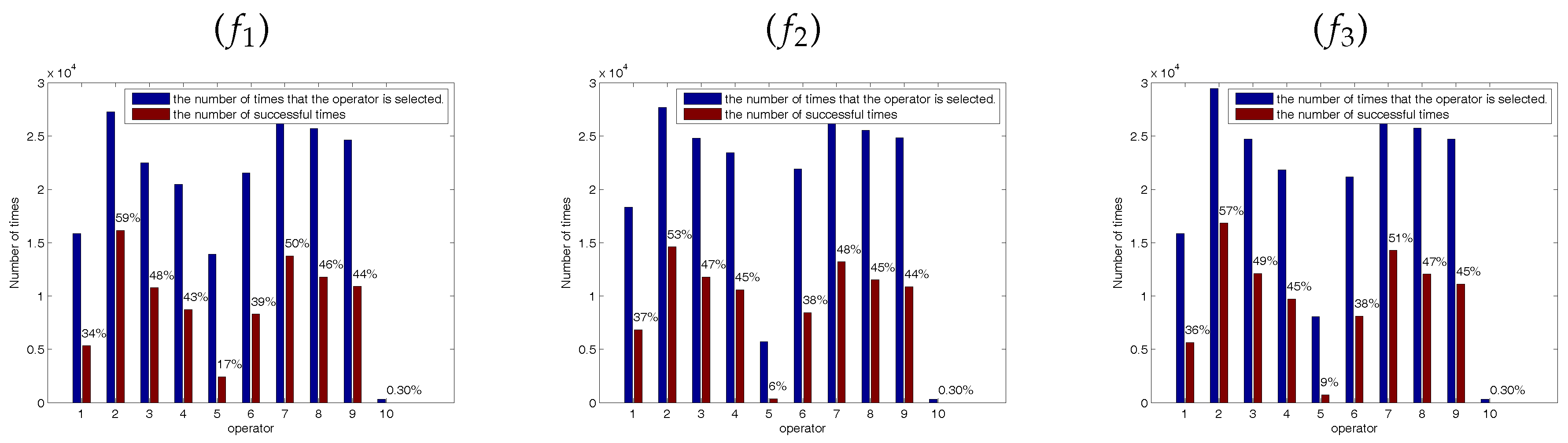
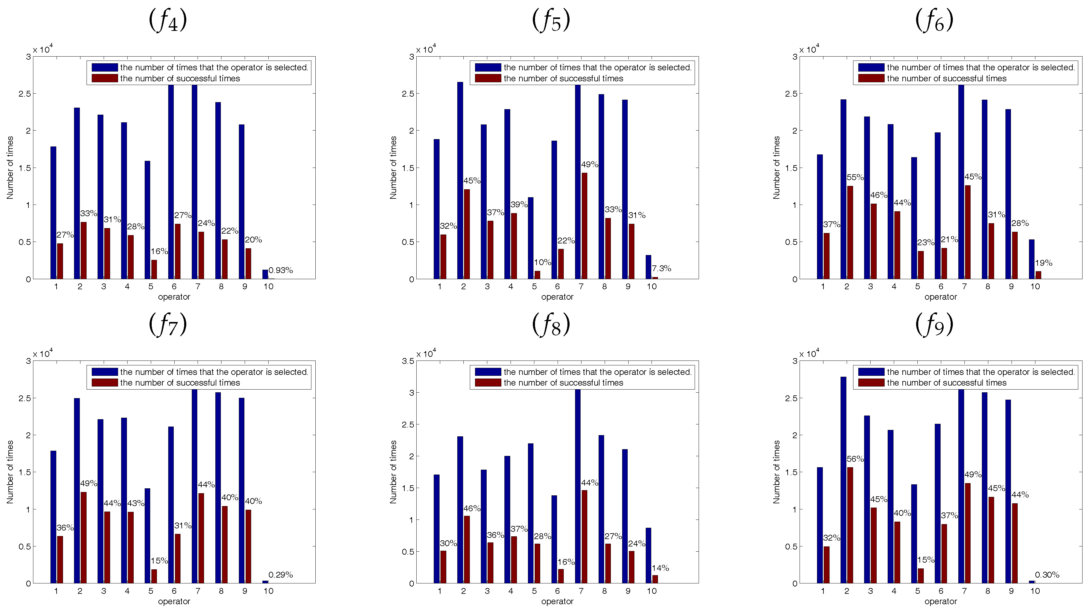
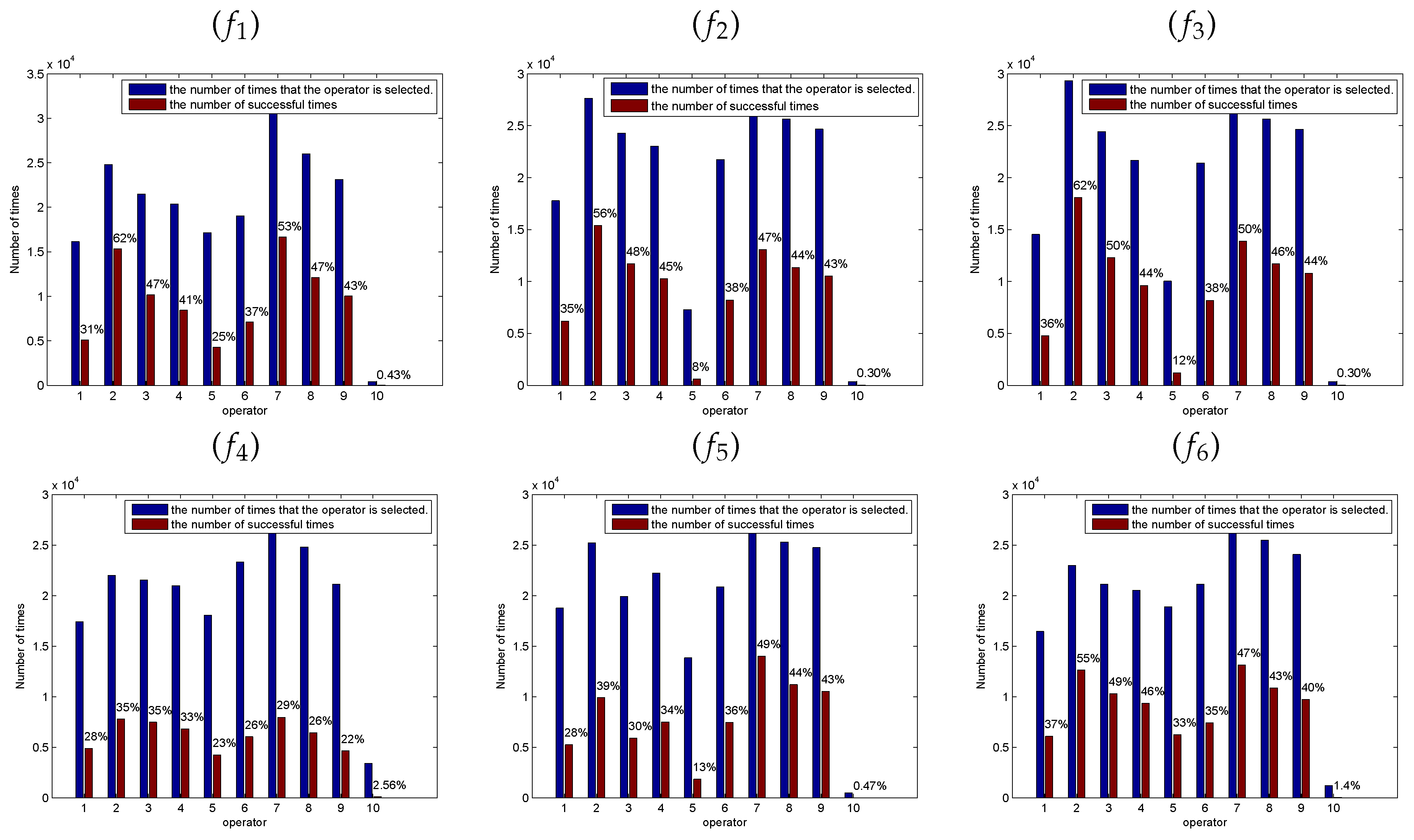
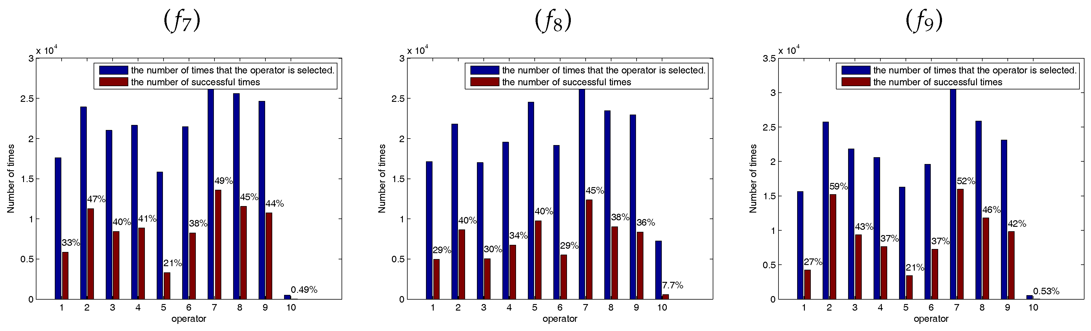
Figure 5, Figure 6 and Figure 7 show the success ratio of each SSE. The horizontal ordinate 1–5 correspond to the success ratio of each SSE ($k=1,2,3,4,5$) at the midpoint of the experiments ($Max.FE/2$) and 6–10 correspond to the success ratio of each SSE ($k=1,2,3,4,5$) at the end of the experiments ($Max.FE$). As shown in these figures, the self-learning mechanism selected different SSE in solving different functions and different functions have different optimal combination of SSEs. In the figures, the coordinate 2 is corresponding to the second SSE at the early stage and the coordinate 7 is corresponding to the second SSE at the latter stage. In most of the functions, the second SSE (coordinate 2 and coordinate 7) has the highest success rate and the fifth SSE has the lowest success rate. The second SSE with the global best solution can improve exploitation. At the early stage of the optimization, the bees are inclined to locate the promising regions by wandering through the entire search space. At the latter stage, the bees are busy to fine-tune the present solutions to obtain the global optimal solution. Therefore, these solutions may trap in the local minimum at the latter stage of the optimization process. The fifth SSE is mainly to make the bees escape from the local minimum. Because functions $f1$–$f4$ are unimodal functions, the fifth SSE with lévy flight step-size has a lower success ratio at the latter stage. However, functions $f5$–$f9$ are multimodal functions which have many local minimum in the search space. The higher success ratio indicates that the SSE with lévy flight step-size can escape from the local optimum effectively to improve search efficiency.

4.3. Comparison Regarding the t-Test

This section mainly analyzes the experimental data and study whether the experimental results are statistically significantly different between SLABC and other algorithm. The F-test was used to analyze the homogeneity of variances and two-tailed t-test was used to determine if two sets of data are significantly different from each other. The sample size and number of degrees of freedom were set as 20 and 38, respectively. The confidence level was set to 95%. In the F-test, $F_{0.05}(19,19)=2.17$ and if the F-value is larger than 2.17, the corresponding experimental results are heterogeneity of variance. If the p-value received in the t-test is less than 5%, it illustrates that the corresponding experimental results are significantly different.

Table 5. Results of t-tests between SLABC and the best results of the other algorithms regarding the indexes “Mean” for different benchmark functions.

Functions	Dim.	F-Value	p-Value	Significance	Two-Tailed P
	D = 30	39.930	1.10 × 10${}^{-4}$	YES	0.05
$f_1$	D = 60	29.663	2.80 × 10${}^{-5}$	YES	0.05
	D = 100	60.363	1.74 × 10${}^{-8}$	YES	0.05
	D = 30	14.894	0.022	YES	0.05
$f_2$	D = 60	20.124	1.42 × 10${}^{-3}$	YES	0.05
	D = 100	15.007	4.00 × 10${}^{-5}$	YES	0.05
	D = 30	22.624	1.85 × 10${}^{-11}$	YES	0.05
$f_3$	D = 60	30.264	4.25 × 10${}^{-12}$	YES	0.05
	D = 100	16.090	1.85 × 10${}^{-9}$	YES	0.05
	D = 30	11.457	0.065	NO	0.05
$f_4$	D = 60	11.308	0.086	NO	0.05
	D = 100	11.565	0.700	NO	0.05
	D = 30	-	-	SAME	0.05
$f_5$	D = 60	23.119	0.013	YES	0.05
	D = 100	70.236	2.52 × 10${}^{-11}$	YES	0.05
	D = 30	-	-	SAME	0.05
$f_6$	D = 60	10.391	0.039	YES	0.05
	D = 100	5.069	0.251	NO	0.05
	D = 30	44.281	2.27 × 10${}^{-9}$	YES	0.05
$f_7$	D = 60	34.994	1.13 × 10${}^{-15}$	YES	0.05
	D = 100	26.974	8.50 × 10${}^{-16}$	YES	0.05
	D = 30	-	-	SAME	0.05
$f_8$	D = 60	4.813	0.288	NO	0.05
	D = 100	14.296	0.028	YES	0.05
	D = 30	-	-	SAME	0.05
$f_9$	D = 60	23.131	8.40 × 10${}^{-5}$	YES	0.05
	D = 100	27.521	4.32 × 10${}^{-7}$	YES	0.05

lists the results of t-tests between SLABC and the best results of the other algorithms regarding the indexes “Mean” for different benchmark functions (listed are the F-value, p-value, and the significance of the results). “YES” indicates that the experimental results are significantly different between SLABC and the best one in other algorithms. “NO” suggests that no significant difference between the results of SLABC and of other algorithms.

From Table 2, Table 3, Table 4 and Table 5, although other algorithms (distABC) have higher solution accuracy on function $f4$ with $D=30,60,100$, there exist no significant difference between SLABC and distABC. The same as function $f6$ with $D=100$ and function $f8$ with $D=60$, there exist no significant difference between SLABC and other algorithm. Moreover, SLABC and other algorithm obtain the same optimal solution on functions $f5,f6,f8$ with $D=30$.

Based on the results of statistical tests in Table 5, almost most of the results have obvious differences and it is clear that the results of SLABC algorithm are significantly better than the results of other algorithms.

5. Discussion

In the previous sections, comparative results of ABC, GABC, MABC and distABC were presented. In this section, we offer a thorough analysis on the proposed SLABC algorithm and all the algorithms were tested using the same parameters with Section 4.

When constructing the SSE, the value range of the coefficients were adjusted to improve the performance of the SLABC algorithm. This section constructed two SLABC algorithm variants (SLABC1, SLABC2) and experiments on a set of 6 benchmark functions were carried out to clearly show how these coefficients influence the performance in various optimization problems. In SLABC1, the value range of the coefficient $c_1,c_2,c_3,c_4,c_5$ are reduced to half of the corresponding value range in SLABC. In SLABC2, the value range of the coefficient $c_1,c_2,c_3,c_4,c_5$ are increased to double of the corresponding value range in SLABC. The new generated candidate solutions can appear in a large range using the SLABC2 algorithm and can appear in a small range using the SLABC1 algorithm. From

Table 6. Comparison between SLABC and other algorithms for 20 times independent runs tested on 6 basic benchmark functions with 60 dimensions.

Functions	Metrics	SLABC1	SLABC2	SLABC3	SLABC4	SLABC
	Best	3.64 × 10${}^{-30}$	2.41 × 10${}^{-25}$	2.53 × 10${}^{-31}$	2.35 × 10${}^{-30}$	1.99 × 10${}^{-29}$
	Median	7.91 × 10${}^{-29}$	1.67 × 10${}^{-24}$	1.27 × 10${}^{-30}$	9.15 × 10${}^{-30}$	8.70 × 10${}^{-29}$
$f_1$	Worst	1.45 × 10${}^{-27}$	8.14 × 10${}^{-24}$	1.85 × 10${}^{-29}$	3.80 × 10${}^{-29}$	4.59 × 10${}^{-28}$
	Mean	2.22 × 10${}^{-28}$	2.10 × 10${}^{-24}$	4.10 × 10${}^{-30}$	1.18 × 10${}^{-29}$	1.25 × 10${}^{-28}$
	Std	3.80 × 10${}^{-28}$	2.04 × 10${}^{-24}$	5.43 × 10${}^{-30}$	9.38 × 10${}^{-30}$	1.06 × 10${}^{-28}$
	Best	1.40 × 10${}^{-60}$	1.16 × 10${}^{-54}$	1.47 × 10${}^{-63}$	9.24 × 10${}^{-63}$	1.79 × 10${}^{-61}$
	Median	2.55 × 10${}^{-59}$	3.53 × 10${}^{-53}$	3.48 × 10${}^{-62}$	1.21 × 10${}^{-61}$	5.17 × 10${}^{-60}$
$f_2$	Worst	2.09 × 10${}^{-57}$	8.46 × 10${}^{-52}$	1.04 × 10${}^{-60}$	3.52 × 10${}^{-60}$	2.17 × 10${}^{-58}$
	Mean	3.02 × 10${}^{-58}$	8.29 × 10${}^{-53}$	1.48 × 10${}^{-61}$	6.99 × 10${}^{-61}$	2.75 × 10${}^{-59}$
	Std	5.46 × 10${}^{-58}$	1.85 × 10${}^{-52}$	2.55 × 10${}^{-61}$	1.15 × 10${}^{-60}$	5.94 × 10${}^{-59}$
	Best	5.20 × 10${}^{-16}$	1.49 × 10${}^{-13}$	6.73 × 10${}^{-17}$	2.14 × 10${}^{-16}$	3.23 × 10${}^{-16}$
	Median	7.69 × 10${}^{-16}$	2.31 × 10${}^{-13}$	1.80 × 10${}^{-16}$	3.96 × 10${}^{-16}$	6.49 × 10${}^{-16}$
$f_3$	Worst	1.83 × 10${}^{-15}$	3.98 × 10${}^{-13}$	3.25 × 10${}^{-16}$	6.87 × 10${}^{-16}$	1.24 × 10${}^{-15}$
	Mean	8.93 × 10${}^{-16}$	2.49 × 10${}^{-13}$	1.78 × 10${}^{-16}$	4.14 × 10${}^{-16}$	6.75 × 10${}^{-16}$
	Std	3.85 × 10${}^{-16}$	7.91 × 10${}^{-14}$	7.65 × 10${}^{-17}$	1.26 × 10${}^{-16}$	2.71 × 10${}^{-16}$
	Best	1.00 × 10${}^{-3}$	1.40 × 10${}^{-3}$	4.52 × 10${}^{-2}$	2.54 × 10${}^{-4}$	4.53 × 10${}^{-2}$
	Median	2.91 × 10${}^0$	2.37 × 10${}^0$	5.14 × 10${}^0$	2.12 × 10${}^0$	2.48 × 10${}^0$
$f_4$	Worst	7.04 × 10${}^1$	1.06 × 10${}^2$	1.43 × 10${}^2$	8.68 × 10${}^1$	8.20 × 10${}^1$
	Mean	8.10 × 10${}^0$	1.84 × 10${}^1$	3.30 × 10${}^1$	1.87 × 10${}^1$	1.07 × 10${}^1$
	Std	1.57 × 10${}^1$	3.05 × 10${}^1$	4.12 × 10${}^1$	3.00 × 10${}^1$	2.43 × 10${}^1$
	Best	0.00 × 10${}^0$	0.00 × 10${}^0$	0.00 × 10${}^0$	0.00 × 10${}^0$	0.00 × 10${}^0$
	Median	0.00 × 10${}^0$	0.00 × 10${}^0$	0.00 × 10${}^0$	0.00 × 10${}^0$	0.00 × 10${}^0$
$f_5$	Worst	0.00 × 10${}^0$	0.00 × 10${}^0$	9.95 × 10${}^{-1}$	0.00 × 10${}^0$	0.00 × 10${}^0$
	Mean	0.00 × 10${}^0$	0.00 × 10${}^0$	4.97 × 10${}^{-2}$	0.00 × 10${}^0$	0.00 × 10${}^0$
	Std	0.00 × 10${}^0$	0.00 × 10${}^0$	2.22 × 10${}^{-1}$	0.00 × 10${}^0$	0.00 × 10${}^0$
	Best	0.00 × 10${}^0$	0.00 × 10${}^0$	0.00 × 10${}^0$	0.00 × 10${}^0$	0.00 × 10${}^0$
	Median	2.00 × 10${}^{-14}$	0.00 × 10${}^0$	0.00 × 10${}^0$	0.00 × 10${}^0$	0.00 × 10${}^0$
$f_6$	Worst	1.35 × 10${}^{-4}$	6.66 × 10${}^{-16}$	8.99 × 10${}^{-14}$	1.11 × 10${}^{-16}$	6.66 × 10${}^{-16}$
	Mean	9.21 × 10${}^{-6}$	3.33 × 10${}^{-17}$	4.50 × 10${}^{-15}$	5.55 × 10${}^{-18}$	5.55 × 10${}^{-17}$
	Std	3.16 × 10${}^{-5}$	1.49 × 10${}^{-16}$	2.01 × 10${}^{-14}$	2.48 × 10${}^{-17}$	1.75 × 10${}^{-16}$

, the SLABC2 is worse than SLABC and SLABC1, which shows that the increased value range reduced the performance of the SLABC algorithm. Moreover, SLABC is better than SLABC1 except function $f_4$, which means that too small value range can reduce solution accuracy. Through the analysis of experimental data, the changes of the value range can influence the performance of SLABC algorithm and only the appropriate value range can generate the better solutions.

Five SSEs are used to solve the optimization problem and each SSE has different effect. For example, the fifth SSE with Lévy flight step-size can help the artificial bees escape from the local optimum effectively. However, when solving the optimization problem of unimodal function, the fifth SSE is ineffective. This section constructed another SLABC algorithm variants (SLABC3 without the fifth SSEs) to illustrate the effect of such combination. As can be seen from Table 6, SLABC3 obtained the better solution than SLABC on the unimodal functions $f_1,f_2,f_3$. Therefore, we can choose combination of different SSEs to solve different optimization problems in the future applications.

In order to avoid the interference between the early stage and the latter stage, SLABC algorithm divides the whole optimization process into two stages. We can divide the optimization process into much more stages to further reduce interference between each stage. To show the effect of such division, this section constructed another SLABC algorithm variants (SLABC4) which divides the whole optimization process into ten stages. As can be seen from Table 6, SLABC4 obtained the better solution than SLABC on most of the functions. Dividing the optimization process into several stages can improve the performance of SLABC algorithm and how to divide the optimization process remains to be a problem should be further studied.

This paper proposes a self-learning mechanism to select the appropriate SSE according to the previous success ratio. Such mechanism is a reinforcement mechanism and other optimization algorithms can construct novel algorithms variants to improve the performance by using the self-learning mechanism.

6. Conclusions

This paper proposes an improved ABC algorithm based on the self-learning mechanism with five SSEs as the candidate operator pool. Among them, one SSE is good at exploration; other two SSEs are good at exploitation; another SSE intends to balance the two aspects. The last SSE with Lévy flight step-size can avoid trapping in local optimal solution. Meanwhile, a simple self-learning mechanism is proposed, wherein the SSE is selected according to the previous success ratio in generating promising solutions at each iteration. Experiments verify that the proposed SLABC algorithm can improve search efficiency and speed up the convergence rate.

References

- Karaboga, D. An Idea Based on Honey Bee Swarm for Numerical Optimization; Technical Report TR06; Erciyes University: Kayseri, Turkey, 2005. [Google Scholar]
- Karaboga, D.; Basturk, B. A powerful and efficient algorithm for numerical function optimization: Artificial bee colony (ABC) algorithm. J. Glob. Optim. 2007, 39, 459–471. [Google Scholar] [CrossRef]
- Mirjalili, S.; Mirjalili, S.M.; Lewis, A. Let a biogeography-based optimizer train your Multi-Layer Perceptron. Inf. Sci. 2014, 269, 188–209. [Google Scholar] [CrossRef]
- Zorarpacı, E.; Özel, S.A. A hybrid approach of differential evolution and artificial bee colony for feature selection. Expert Syst. Appl. 2016, 62, 91–103. [Google Scholar] [CrossRef]
- Das, R.; Akay, B.; Singla, R.K.; Singh, K. Application of artificial bee colony algorithm for inverse modelling of a solar collector. Inverse Probl. Sci. Eng. 2016, 25, 887–908. [Google Scholar] [CrossRef]
- Marzband, M.; Azarinejadian, F.; Savaghebi, M.; Guerrero, J.M. An Optimal Energy Management System for Islanded Microgrids Based on Multiperiod Artificial Bee Colony Combined With Markov Chain. IEEE Syst. J. 2017, 11, 1712–1722. [Google Scholar] [CrossRef]
- Luo, J.; Liu, Q.; Yang, Y.; Li, X.; rong Chen, M.; Cao, W. An artificial bee colony algorithm for multi-objective optimisation. Appl. Soft Comput. 2017, 50, 235–251. [Google Scholar] [CrossRef]
- Lozano, M.; García-Martínez, C.; Rodríguez, F.J.; Trujillo, H.M. Optimizing network attacks by artificial bee colony. Inf. Sci. 2017, 377, 30–50. [Google Scholar] [CrossRef]
- Sonmez, M.; Akgüngör, A.P.; Bektaş, S. Estimating transportation energy demand in Turkey using the artificial bee colony algorithm. Energy 2017, 122, 301–310. [Google Scholar] [CrossRef]
- Zhou, J.; Yao, X. Multi-population parallel self-adaptive differential artificial bee colony algorithm with application in large-scale service composition for cloud manufacturing. Appl. Soft Comput. 2017, 56, 379–397. [Google Scholar] [CrossRef]
- Sundar, S.; Suganthan, P.N.; Jin, C.T.; Xiang, C.T.; Soon, C.C. A hybrid artificial bee colony algorithm for the job-shop scheduling problem with no-wait constraint. Soft Comput. 2017, 21, 1193–1202. [Google Scholar] [CrossRef]
- Woźniak, M.; Połap, D. Bio-inspired methods modeled for respiratory disease detection from medical images. Swarm Evol. Comput. 2018, in press. [Google Scholar] [CrossRef]
- Bansal, J.C.; Sharma, H.; Arya, K.V.; Nagar, A. Memetic search in artificial bee colony algorithm. Soft Comput. 2013, 17, 1911–1928. [Google Scholar] [CrossRef]
- Kang, F.; Li, J.; Li, H. Artificial bee colony algorithm and pattern search hybridized for global optimization. Appl. Soft Comput. 2013, 13, 1781–1791. [Google Scholar] [CrossRef]
- Gao, W.; Liu, S.; Huang, L. Enhancing artificial bee colony algorithm using more information-based search equations. Inf. Sci. 2014, 270, 112–133. [Google Scholar] [CrossRef]
- Zhou, X.; Wang, H.; Wang, M.; Wan, J. Selection Mechanism in Artificial Bee Colony Algorithm: A Comparative Study on Numerical Benchmark Problems. In Neural Information Processing; Springer: Cham, Switzerland, 2017; pp. 61–69. [Google Scholar]
- Kennedy, J.; Eberhart, R. Particle swarm optimization. In Proceedings of the IEEE International Conference on Neural Networks, Perth, WA, Australia, 27 November–1 December 1995; Volume 4, pp. 1942–1948. [Google Scholar]
- Zhu, G.; Kwong, S. Gbest-guided artificial bee colony algorithm for numerical function optimization. Appl. Math. Comput. 2010, 217, 3166–3173. [Google Scholar] [CrossRef]
- Storn, R.; Price, K. Differential Evolution—A Simple and Efficient Heuristic for Global Optimization over Continuous Spaces. J. Glob. Optim. 1997, 11, 341–359. [Google Scholar] [CrossRef]
- Gao, W.; Liu, S. Improved artificial bee colony algorithm for global optimization. Inf. Process. Lett. 2011, 111, 871–882. [Google Scholar] [CrossRef]
- Gao, W.; Liu, S. A modified artificial bee colony algorithm. Comput. Oper. Res. 2012, 39, 687–697. [Google Scholar] [CrossRef]
- Akay, B.; Karaboga, D. A modified Artificial Bee Colony algorithm for real-parameter optimization. Inf. Sci. 2012, 192, 120–142. [Google Scholar] [CrossRef]
- Gao, W.; Liu, S.; Huang, L. A Novel Artificial Bee Colony Algorithm Based on Modified Search Equation and Orthogonal Learning. IEEE Trans. Cybern. 2013, 43, 1011–1024. [Google Scholar] [PubMed]
- Babaoglu, I. Artificial bee colony algorithm with distribution-based update rule. Appl. Soft Comput. 2015, 34, 851–861. [Google Scholar] [CrossRef]
- Ratnaweera, A.; Halgamuge, S.K.; Watson, H.C. Self-organizing hierarchical particle swarm optimizer with time-varying acceleration coefficients. IEEE Trans. Evol. Comput. 2004, 8, 240–255. [Google Scholar] [CrossRef]
- Viswanathan, G.M.; Buldyrev, S.V.; Havlin, S.; Da, L.M.; Raposo, E.P.; Stanley, H.E. Optimizing the success of random searches. Nature 1999, 401, 911–914. [Google Scholar] [CrossRef] [PubMed]
- Viswanathan, G.M.; Afanasyev, V.; Buldyrev, S.V.; Murphy, E.J.; Prince, P.A.; Stanley, H.E. Lévy flight search patterns of wandering albatrosses. Nature 1996, 381, 413–415. [Google Scholar] [CrossRef]
- Edwards, A.M.; Phillips, R.A.; Watkins, N.W.; Freeman, M.P.; Murphy, E.J.; Afanasyev, V.; Buldyrev, S.V.; Da, L.M.; Raposo, E.P.; Stanley, H.E. Revisiting Lévy flight search patterns of wandering albatrosses, bumblebees and deer. Nature 2007, 449, 1044–1048. [Google Scholar] [CrossRef] [PubMed] [Green Version]
- Reynolds, A.M.; Frye, M.A. Free-flight odor tracking in Drosophila is consistent with an optimal intermittent scale-free search. PLoS ONE 2007, 2, e354. [Google Scholar] [CrossRef] [PubMed]
- Mantegna, R.N. Fast, accurate algorithm for numerical simulation of Lévy stable stochastic processes. Phys. Rev. E 1994, 49, 4677–4683. [Google Scholar] [CrossRef]
Figure 1.
An example of 1000 steps of a Lévy flight in two dimensions. The origin of the motion is at [0,0], the step-size is generated according to Equation (5) with and the angular direction is uniformly distributed.
Figure 2.
Comparison of the convergence results of the average best solution with 30 dimensions. () Sphere Function; () Quartic Function; () Schwefel’s Problem 2.22; () Rosenbrock Function; () Rastrigin Function; () Griewank Function; () Ackley Function; () Schwefel’s Problem 2.26; () Penalized Function.
Figure 3.
Comparison of the convergence results of the average best solution with 60 dimensions. () Sphere Function; () Quartic Function; () Schwefel’s Problem 2.22; () Rosenbrock Function; () Rastrigin Function; () Griewank Function; () Ackley Function; () Schwefel’s Problem 2.26; () Penalized Function.
Figure 4.
Comparison of the convergence results of the average best solution with 100 dimensions. () Sphere Function; () Quartic Function; () Schwefel’s Problem 2.22; () Rosenbrock Function; () Rastrigin Function; () Griewank Function; () Ackley Function; () Schwefel’s Problem 2.26; () Penalized Function.
Figure 5.
The success ratio of each SSE (operator). The horizontal ordinate denotes success ratio of each solution search equation at the midpoint of the experiments () and the end of the experiments () with 30 dimensions. () Sphere Function; () Quartic Function; () Schwefel’s Problem 2.22; () Rosenbrock Function; () Rastrigin Function; () Griewank Function; () Ackley Function; () Schwefel’s Problem 2.26; () Penalized Function.
Figure 6.
The success ratio of each SSE. The horizontal ordinate denotes success ratio of each solution search equation (operator) at the midpoint of the experiments () and the end of the experiments () with 60 dimensions. () Sphere Function; () Quartic Function; () Schwefel’s Problem 2.22; () Rosenbrock Function; () Rastrigin Function; () Griewank Function; () Ackley Function; () Schwefel’s Problem 2.26; () Penalized Function.
Figure 7.
The success ratio of each SSE. The horizontal ordinate denotes success ratio of each solution search equation (operator) at the midpoint of the experiments () and the end of the experiments () with 100 dimensions. () Sphere Function; () Quartic Function; () Schwefel’s Problem 2.22; () Rosenbrock Function; () Rastrigin Function; () Griewank Function; () Ackley Function; () Schwefel’s Problem 2.26; () Penalized Function.