A Self-Adaptive Evolutionary Algorithm for the Berth Scheduling Problem: Towards Efficient Parameter Control


Department of Civil & Environmental Engineering, Florida A&M University-Florida State University, Tallahassee, FL 32310-6046, USA
*
Author to whom correspondence should be addressed.
Algorithms 2018, 11(7), 100; https://doi.org/10.3390/a11070100
Submission received: 5 May 2018
/
Revised: 25 June 2018
/
Accepted: 28 June 2018
/
Published: 3 July 2018
Abstract
:Since ancient times, maritime transportation has played a very important role for the global trade and economy of many countries. The volumes of all major types of cargo, which are transported by vessels, has substantially increased in recent years. Considering a rapid growth of waterborne trade, marine container terminal operators should focus on upgrading the existing terminal infrastructure and improving operations planning. This study aims to assist marine container terminal operators with improving the seaside operations and primarily focuses on the berth scheduling problem. The problem is formulated as a mixed integer linear programming model, minimizing the total weighted vessel turnaround time and the total weighted vessel late departures. A self-adaptive Evolutionary Algorithm is proposed to solve the problem, where the crossover and mutation probabilities are encoded in the chromosomes. Numerical experiments are conducted to evaluate performance of the developed solution algorithm against the alternative Evolutionary Algorithms, which rely on the deterministic parameter control, adaptive parameter control, and parameter tuning strategies, respectively. Results indicate that all the considered solution algorithms demonstrate a relatively low variability in terms of the objective function values at termination from one replication to another and can maintain the adequate population diversity. However, application of the self-adaptive parameter control strategy substantially improves the objective function values at termination without a significant impact on the computational time.
1. Introduction
Marine transportation has been playing a critical role for the global trade since ancient times [1]. By 1200 BCE, Egyptian vessels were able to support trade on the maritime routes that were leading to Sumatra (an island, located near Indonesia), which were considered to be the longest trade routes of that time [1]. Chinese merchants initiated the regional maritime trade networks in the South China Sea and the Indian Ocean towards the 10th century. European countries (including Spain, England, Portugal, the Netherlands, and France) established the global maritime trade network in 16th century [1]. Supported by new technologies [2,3,4], maritime trade networks rapidly expanded all over the globe. By 2006, waterborne trade accounted for ≈90% of global international trade by volume and ≈70% by value.
Increasing waterborne trade tendencies have been observed after 2006. Based on a recent report, released by the United Nations Conference on Trade and Development in 2017, the total volumes of waterborne trade increased by 33.6% from 7.7 billion tons in 2006 to 10.3 billion tons in 2016 [5]. Moreover, the volumes of all major types of cargo, transported by vessels, have significantly increased over the last ten years. Specifically, containerized trade increased by 59.9%, while major bulk cargo, dry bulk cargo, and oil/gas increased by 74.9%, 10.8%, and 13.2%, respectively, from 2006 to 2016. The general consumption goods and high-value cargo are typically transported in containerized form. Containers are transferred among different continents by vessels, which are served at marine container terminals (MCTs). Rapid growth of waterborne trade requires MCT operators upgrading the existing terminal infrastructure and improving operations planning.
MCT operations can be categorized in the following three types [1,6]: (1) seaside operations, which focus on service of arriving vessels (i.e., loading containers on vessels and unloading containers from vessels); (2) marshaling yard operations, which focus on temporary storage of containers in yard blocks of the MCT marshaling yard; and (3) landside operations, which focus on pick-up and delivery of containers by the inland transportation modes (generally, on-dock rail and/or drayage trucks). Efficient seaside operations are critical for MCT performance, as disruptions in the seaside operations may significantly delay service of the arriving vessels. A significant amount of previously conducted studies primarily focused on the berth scheduling problem (BSP), aiming to improve the seaside operations at MCTs [6]. In BSP, the MCT operator aims to assign arriving vessels for service at available MCT berthing positions and determine the service order of vessels at each berthing position.
The BSP is a challenging decision problem, which can be reduced to the unrelated machine scheduling problem [6,7,8,9,10,11,12]. As underlined by Pinedo [13], the unrelated machine scheduling problem (therefore, the BSP as well) has NP-hard complexity. Hence, the realistic size problem instances of BSPs typically cannot be solved using the exact optimization algorithms to the global optimality within an acceptable computational time. To obtain good-quality berth schedules within a reasonable computational time, many different heuristic and metaheuristic algorithms have been presented in the BSP literature. For a detailed review of the BSP mathematical models and solution algorithms this study refers to the literature survey, conducted by Bierwirth and Meisel [6]. Many BSP studies applied Evolutionary Algorithms (EAs) and demonstrated their efficiency based on the numerical experiments [6,7,8,9,10,11,12,14,15,16,17,18,19]. EAs are biologically inspired metaheuristics, where the candidate solutions to the problem of interest are encoded in the chromosomes [20,21]. At the beginning, a typical EA initializes the population, represented by a group of chromosomes, and evaluates fitness (i.e., quality of the solutions) of the initial population chromosomes. After that, the EA starts an iterative procedure, where the chromosomes are continuously changed by applying specific EA operators (i.e., parent selection, crossover, mutation, offspring selection) with the main objective to discover superior solutions. The iterative procedure is terminated once the EA satisfies a specific convergence criterion.
Each EA has several parameters, including population size (i.e., the number of chromosomes in the population), crossover probability, mutation probability, selection operator parameters, and others. There are two approaches for selection of the EA parameters [20,21,22], including the following (see Figure 1): (1) parameter tuning; and (2) parameter control. Note that the aforementioned approaches can be used to set parameters not only for EAs, but also for the other heuristic and metaheuristic algorithms. As for the parameter tuning approach, different values of each parameter are evaluated for a given EA, and the best parameter values are selected based on the analysis of a tradeoff between the objective function and computational time values (the latter analysis is referred to as the “parameter tuning” analysis). The parameter tuning approach assumes that the selected parameter values remain unchanged throughout the algorithmic run.
On the other hand, the parameter control approach adjusts the values of EA parameters throughout the algorithmic run based on certain strategies. There are three common types of the parameter control strategies [20,21,22], including the following (see Figure 1): (1) deterministic—the algorithmic parameters are altered based on a certain counter (e.g., computational time, number of generations) without any feedback from the search; (2) adaptive—the algorithmic parameters are altered based on feedback from the search (e.g., behavior of the objective/fitness function); and (3) self-adaptive—the algorithmic parameters are encoded in the chromosomes and evolve throughout the algorithmic run.
The EAs, presented in the BSP literature, primarily rely on the parameter tuning strategy. In some of the recent BSP studies, the deterministic and adaptive parameter control strategies were implemented within the proposed EAs [10,12]. Both deterministic and adaptive parameter control strategies were found to be promising and outperformed the parameter tuning strategy. Specifically, the EAs with parameter control can more efficiently move along the search space, identify promising domains of the search space, and exploit the identified domains for superior solutions [10,12]. On the other hand, setting constant parameter values, which do not change throughout the algorithmic run (i.e., the parameter tuning strategy), typically limits the explorative and exploitative EA capabilities. Although the self-adaptive parameter control strategy has been used in the EA literature [20,21,22], none of the published to date studies applied such parameter control strategy for the BSP. The contributions of this study to the state-of-the-art can be summarized as follows:
- (1)
- A novel self-adaptive EA is proposed for the BSP, where the crossover and mutation probabilities are encoded in the chromosomes and evolve throughout the algorithmic run;
- (2)
- A novel heuristic is presented for the population initialization, which accounts for the spatial requirements in berth scheduling;
- (3)
- A comprehensive comparative analysis is conducted to evaluate the EA with self-adaptive parameter control strategy against the alternative EAs, which rely on the deterministic parameter control, adaptive parameter control, and parameter tuning strategies, respectively; and
- (4)
- The major algorithmic performance indicators are considered, including objective function and computational time values, convergence patterns, evolution of the self-adaptive algorithmic parameter values, algorithmic stability, and changes in the population diversity.
The remaining sections of this manuscript are structured in the following manner. Section 2 provides a detailed description of the BSP studied herein, while Section 3 presents a mixed integer linear mathematical model for the problem. Section 4 outlines the main steps of the developed self-adaptive EA and provides a detailed description of each step. Section 5 focuses on a detailed complexity analysis of the developed self-adaptive EA. Section 6 describes the numerical experiments, which were conducted throughout this study to evaluate performance of the proposed solution algorithm. The last section summarizes findings of this study and discusses potential extensions, which can be explored as a part of the future research.
2. MCT Operations Description
This study focuses on modeling the seaside operations at a multi-user MCT, where vessels from different liner shipping companies deliver and pick up containers. Various MCT berthing layouts have been reported in the BSP literature (including discrete, continuous, hybrid, indented, and channel) [6,17], and the commonly used discrete berthing layout will be adopted in this study for the considered MCT. Based on the discrete berthing layout, the MCT wharf is partitioned in a set of berthing positions, which will be referred to as , and one vessel can be moored at a given berthing position at the time. The MCT layout, which will be modeled in this study, is presented in Figure 2. Let be a set of arriving vessels, which must be served at the MCT.
There are two common types of vessel arrivals, which have been modeled in the BSP literature, including the following [6]: (a) static vessel arrivals—all vessels have already arrived at the MCT, and the berth schedule should be designed based on the specific objectives; and (b) dynamic vessel arrivals—vessels have not arrived at the MCT yet, but the MCT operator has the information regarding the expected vessel arrival time (which is negotiated with the corresponding liner shipping company). The dynamic vessel arrivals will be considered in this study. The vessels are assumed to arrive at the MCT at the scheduled time (—measured in h). The scope of this study does not include modeling uncertainty in vessel arrivals due to different factors, including adverse weather, reduction in the vessel sailing speed as a result of the main engine malfunctioning, potential delays in vessel service at preceding ports, human errors, and others.
Upon arrival at the MCT, each vessel will be towed by tug boats to the assigned MCT berthing position. In some cases, the assigned berthing position may not be available at the moment (as the other vessel is being served), and the vessel will be towed to the dedicated waiting area, which is located near the MCT. Note that increasing waiting time (—measured in h) of vessels may negatively affect the MCT operations, as increasing number of waiting vessels may cause congestion in the access channel and result in navigational difficulties for the vessels, entering and leaving the MCT. The MCT operator should consider the length (—measured in ft.) and draft (—measured in ft.) of the arriving vessels in the design of berth schedules. Each berthing position has two spatial attributes, including length (—measured in ft.) and depth (—measured in ft.). If vessel does not satisfy certain horizontal and vertical clearance requirements (which will be denoted as and , respectively, and are both measured in ft.), it cannot be assigned for service at berthing position . Moreover, service of a given vessel cannot start before the time, when the assigned berthing position becomes available in the planning horizon at the first time (—measured in h). Once the assigned berthing position becomes available, the vessel is moored, and the on-shore quay cranes start loading and unloading containers (see Figure 2).
There are several other important factors, which should be considered by the MCT operator in the design of berth schedules, including the following: (1) vessel handling rates; (2) allocation of the available handling equipment; and (3) allocation of the available storage space. Vessel handling rates, measured in the number of twenty-foot equivalent units (TEUs) handled per hour, are negotiated between the MCT operator and liner shipping companies. To provide the negotiated vessel handling rates, the MCT operator has to allocate the required amount of handling equipment for each vessel, including quay cranes for loading containers on the vessel and unloading containers from the vessel, internal transport vehicles (e.g., yard trucks, automated guided vehicles, straddle carriers, automated lifting vehicles) for transfer of containers from the seaside to the marshaling yard, gantry cranes for handling containers in the marshaling yard, and other miscellaneous equipment. The handling time of vessel at berthing position (—measured in h) is determined based on the number of containers to be handled for vessel and the handling productivity, negotiated with the liner shipping company.
Furthermore, the MCT operator must allocate the storage space in the marshaling yard for containers, delivered by each vessel. Generally, the storage space is allocated as close as possible to the berthing position, where a given vessel is originally planned to be assigned for service (the latter term is also known as “preferred berthing position” in the BSP literature [6,11]). Because of changes in the original berth schedule, a given vessel may be assigned for service at an alternative berthing position (e.g., to reduce the waiting time of that vessel in case if its “preferred berthing position” is occupied by another vessel at the moment). Due to changes in the original berth assignment, the vessel handling time will increase since the internal transport vehicles will be required to travel longer distances between the alternative berthing position and the assigned storage space in the marshaling yard (as compared to the travel distance between the “preferred berthing position” and the assigned storage space).
Based on the contractual agreement with the MCT operator, the liner shipping company requests a specific departure time (—measured in h). It is critical for the liner shipping company to ensure that each vessel will leave the MCT at the scheduled time to avoid potential delays at the consecutive ports, which must be visited by that vessel. The MCT operator may be even expected to pay penalties to the liner shipping company in case of late vessel departures [6]. To design an efficient berth schedule, the MCT operator must account for priority of the arriving vessels. The priority of vessels will be assigned using weights (—a real-valued number, varying from 0.10 to 1.00). The latter methodology has been widely used in the BSP literature [6]. The overall objective of the MCT operator is to develop the optimal berth schedule, which will allow minimizing the total weighted vessel waiting time, the total weighted vessel handling time, and the total weighted vessel late departures.
3. Model Formulation
This section of the manuscript focuses on description of the nomenclature that will be used throughout this study and presents a mixed integer linear mathematical model for the discrete dynamic berth scheduling problem with spatial requirements (BSPSR). A detailed description of the BSPSR mathematical model components is presented in Table 1.
The objective function (1) of the BSPSR mathematical model, denoted as , aims to minimize the total weighted turnaround time of vessels (which is composed of the total weighted vessel waiting and handling times) and the total weighted vessel late departures.
Constraint set (2) indicates that no more than one vessel can be served at each berthing position at the time.
Constraint set (3) guarantees that each vessel will be assigned to one of the available berthing positions in any service order.
Constraint sets (4) and (5) ensure that the horizontal and vertical clearance requirements will not be violated for each vessel moored at one of the MCT berthing positions.
Constraint set (6) guarantees that service of each vessel will start after its arrival at the MCT.
Constraint set (7) calculates the start service time for each vessel calling the MCT.
Constraint set (8) computes the waiting time of each vessel before its service start at the MCT.
Constraint set (9) computes the finish service time for each vessel calling the MCT.
Constraint set (10) estimates the late departure hours for each vessel calling the MCT.
Constraint sets (11)–(13) define the nature of decision variables, auxiliary variables, and parameters of the BSPSR mathematical model.
4. Design of a Self-Adaptive Evolutionary Algorithm
This section of the manuscript focuses on a detailed description of the self-adaptive EA (SAEA), which was developed to solve the realistic size problem instances of the BSPSR mathematical model within an acceptable computational time. Unlike typical EAs, the proposed SAEA algorithm deploys a self-adaptive parameter control strategy, where the crossover and mutation probabilities (which are considered to be the major EA parameters [20,21]) are encoded in the chromosomes and change throughout evolution of the algorithm from one generation to another. The main SAEA steps are presented in Section 4.1 of the manuscript, while a detailed description of each SAEA step is presented in Section 4.2, Section 4.3, Section 4.4, Section 4.5, Section 4.6, Section 4.7, Section 4.8 and Section 4.9 of the manuscript.
4.1. The Main SAEA Steps
Figure 3 presents the main SAEA steps. At the beginning, the data structures are initialized for the required BSPSR and SAEA parameters (step 0). Also, in step 0, the SAEA algorithm starts the generation count (). In the next steps, the initial population is created (step 1), and fitness of the initial population is evaluated (step 2). After that, the algorithm enters the main loop and updates the generation count (step 3). Next, the parent selection is executed to identify the population chromosomes that will participate in the SAEA operations (step 4). Then, the offspring chromosomes are produced as a result of applying the SAEA algorithmic operators to the parent chromosomes (step 5). Also, in step 5, the repairing operator is executed to repair the infeasible offspring, which were produced as a result of the SAEA operations (if any). Fitness of the repaired offspring chromosomes is evaluated in step 6. Then, the offspring chromosomes for the next generation are determined (step 7). The SAEA algorithm is terminated once the maximum allowable number of generations () has been reached (which will be set as a termination criterion). When the algorithm is terminated, it will return the best solution, which corresponds to the berth schedule with the least possible sum of the total weighted vessel turnaround time and the total weighted vessel late departures.
4.2. Representation of Solutions
Chromosomes (or individuals) are used in EAs to represent a solution to a given problem [20,21]. A hybrid chromosome representation will be adopted in this study, where one part of the chromosome will be represented using integers, while the other part will be represented using real-valued numbers. The first part of each chromosome, which contains integer numbers, will be used to denote the vessel to berthing position to service order assignment (i.e., the BSPSR solution). The second part of each chromosome, which contains real-valued numbers, will be used to denote the crossover and mutation probabilities (that will be referred to as and , respectively). The chromosome components (e.g., berthing position identifiers, vessel identifiers, crossover and mutation probabilities) will be referred to as “genes” [20]. Location of a gene along the chromosome will be referred to as “locus” [20]. Value of a gene will be referred to as “allele” [20]. The adopted chromosome representation is not common among canonical EAs, which have been used in the BSP literature, as the proposed SAEA applies the self-adaptive parameter control strategy. An example of the SAEA chromosome representation is illustrated in Figure 4.
In the considered example, 8 vessels are scheduled for service at the MCT. Berth “1” is assigned to serve vessels “3”, “2”, and “7” (in that specific service order); on the other hand, berth “2” is assigned to serve vessels “5”, “8”, “1”, “6”, and “4” (in that specific service order). Moreover, the probability of the presented chromosome to undergo a crossover operation (if selected as a parent) is , while the probability of each gene of the presented chromosome to undergo a mutation operation is . The length of each chromosome in the population can be determined as , i.e., summation of the number of vessels, calling for service at the MCT, and “2”, where additional 2 genes are required to store the information regarding the crossover and mutation probabilities.
4.3. Generation of the Initial Chromosomes and Population
The first half of the SAEA population will be initialized randomly (i.e., vessels will be assigned randomly to the MCT berthing positions, while the crossover and mutation probabilities will be generated as random values, ranging between 0.01 and 1.00). The second half of the SAEA population will be initialized using a local search heuristic for the vessel to berthing position to service order assignment, while the crossover and mutation probabilities will be still generated randomly. The local search heuristic is based on the First Come First Served (FCFS) policy. Note that a typical FCFS policy, which has been widely used in the BSP literature, will not be applicable for the BSPSR mathematical model, as it may cause violation of the spatial requirements (i.e., a vessel can be assigned to the berthing position, which does not have sufficient length and/or depth).
This study proposes the FCFS with spatial requirements (FCFS-SR) heuristic, which ensures that the spatial requirements are not violated for the generated berth schedules. The main steps of the FCFS-SR heuristic are outlined in Algorithm 1. Notation is used in Algorithm 1 to represent the updated availability of berthing positions (measured in h), while the rest of notations are adopted from Section 3 of the manuscript. The data structures, required by the FCFS-SR heuristic, are initialized in step 0. Then, the vessels to be served at the MCT are sorted based on their arrival times in step 1. The availability of berthing positions is set equal to the initial availability in step 2. After that, the FCFS-SR heuristic starts an iterative procedure (steps 4–13), where the first available berthing position, which can accommodate the next arriving vessel (and satisfy both horizontal and vertical clearance requirements), is determined in steps 5 and 6. The earliest service order for the first available berthing position is identified in step 7. Then, the vessel is assigned to the first available berthing position, which satisfies both horizontal and vertical clearance requirements, in the earliest service order (step 8). The start and finish vessel service times are estimated in steps 9 and 10. The availability of a berthing position is updated based on the vessel finish service time in step 11. The FCFS-SR heuristic terminates an iterative procedure, once the initial vessel to berthing position to service order assignment is generated for all vessels, calling for service at the MCT.
Note that the FCFS-SR heuristic is deterministic in its nature; therefore, the chromosome portions, which represent vessel to berthing position to service order assignments and are created using FCFS-SR, will be identical. The latter will substantially limit the explorative capabilities at early stages of the SAEA run. To maintain the population diversity and improve the SAEA explorative capabilities, only half of the initial SAEA population will be generated using the FCFS-SR heuristic, while another half will be created randomly (as discussed at the beginning of Section 4.3 of the manuscript). The number of chromosomes in the population (i.e., population size: ) will be established based on the parameter tuning analysis, which is described in Section 6.2 of the manuscript.
| Algorithm 1: First Come First Served with Spatial Requirements (FCFS-SR) Heuristic. |
| - |
| in:—set of vessels; —set of berths; —set of service orders; —berth availability; —vessel arrival times; —vessel handling times; —length of vessels; —length of berths; —horizontal clearance requirements; —draft of vessels; —depth of berths; —vertical clearance requirements |
| out:—initial vessel to berth to service order assignment |
| 0: ; ; ; ; ⊲ Initialization |
| 1: ⊲ Sort the vessels based on their arrival times at the MCT |
| 2: ⊲ Set the initial availability of berthing positions |
| 3: |
| 4: for all do |
| 5: ⊲ Identify potential berthing positions for a vessel |
| 6: ⊲ Select the first available berthing position |
| 7: ⊲ Determine the earliest service order |
| 8: ⊲ Assign a vessel to the first available berthing position in the earliest service order |
| 9: ⊲ Calculate the start vessel service time |
| 10: ⊲ Calculate the finish vessel service time |
| 11: ⊲ Update the availability of a berthing position |
| 12: |
| 13: end for |
| 14: return |
4.4. Fitness Function
Let be a set of individuals in the SAEA population and be a set of generations. The fitness value of individual in generation () is calculated in the developed SAEA algorithm based on the following relationship:
Along with the objective function value of the BSPSR mathematical model (), the fitness function includes the penalty term for violation of the horizontal clearance requirements (, where —horizontal clearance violation penalty, measured in h/ft.; —horizontal clearance violation for individual in generation , measured in ft.) and the penalty term for violation of the vertical clearance requirements (, where —vertical clearance violation penalty, measured in h/ft.; —vertical clearance violation for individual in generation , measured in ft.). The penalty terms are introduced to adjust the fitness function values for infeasible individuals (that violate the horizontal and/or vertical clearance requirements for vessels), which could be generated as a result of the SAEA operations. The horizontal clearance violation for individual in generation can be estimated as a sum of horizontal clearance violations of all vessels that are served at the MCT berthing positions as follows:
The vertical clearance violation for individual in generation can be estimated as a sum of vertical clearance violations of all vessels that are served at the MCT berthing positions as follows:
Based on Equations (15) and (16), chances of the individuals to survive will increase with decreasing degree of violation of horizontal and/or vertical clearance requirements. It is important to set the appropriate values of and penalty terms to ensure that infeasible individuals will have much lower chances to survive as compared to feasible individuals. The appropriate values of penalty terms and will be established based on the parameter tuning analysis, which is described in Section 6.2 of the manuscript.
4.5. Parent Selection Procedure
Once SAEA enters the main loop, it deploys the parent selection procedure to determine the chromosomes that will participate in the SAEA operations and produce the offspring in a given generation. A Roulette Wheel Selection, which has been widely used in canonical Genetic Algorithms and Genetic Programming [20], will be adopted in this study at the parent selection stage. Based on the Roulette Wheel Selection (RWS) mechanism, each individual in the population is assigned a portion of a roulette wheel. A larger portion of the roulette wheel will be assigned to the fittest individual (i.e., the individual with lower objective function value, since the proposed BSPSR mathematical model aims to minimize the total weighted vessel turnaround time and the total weighted vessel late departures). The roulette wheel is continuously rotated, and one individual is selected at each rotation. The chance of a given individual to be selected is proportional to its fitness. The main steps of the RWS mechanism are outlined in Algorithm 2.
The data structures, required by the RWS mechanism, are initialized in step 0. Then, the fitness values of the population chromosomes are adjusted (i.e., values are estimated) in steps 2–5, as the BSPSR mathematical model has a minimization objective function. The adjusted fitness values of the population chromosomes are normalized in step 6 (so, the cumulative population fitness after normalization will be equal to 1.00). After that, RWS starts an iterative procedure (steps 7–11), where a random value between 0.00 and 1.00 is generated in step 8 (i.e., the roulette wheel is rotated). Then, the individual with a normalized fitness value, which is close to the randomly generated value, is selected to become a parent (steps 9 and 10). An iterative procedure is terminated by RWS once the required amount of parent chromosomes has been selected.
| Algorithm 2: Roulette Wheel Selection (RWS). |
| in:—population in generation ; —fitness of chromosomes in generation |
| out:—parent chromosomes in generation |
| 0: ; ; ⊲ Initialization |
| 1: |
| 2: while do |
| 3: ⊲ Adjust the fitness value of a given chromosome |
| 4: |
| 5: end while |
| 6: ⊲ Normalize the adjusted fitness values of the population chromosomes |
| 7: while do |
| 8: ⊲ Generate a random value between 0.00 and 1.00 |
| 9: ⊲ Select the individual based on a randomly generated value |
| 10: ⊲ The selected individual is added to the set of parent chromosomes |
| 11: end while |
| 12: return |
4.6. SAEA Operations
Once the parent chromosomes are selected by the SAEA algorithm, the crossover and mutation operators will be executed to produce and mutate the offspring chromosomes. Two custom operators were designed in this study to perform the crossover and mutation operations for the adopted hybrid chromosome representation, which contains both integer and real-valued genes. A detailed description of the crossover and mutation operations is presented in Section 4.6.1 and Section 4.6.2 of the manuscript, respectively.
4.6.1. Crossover Operation
The crossover operation plays an important role in the design of EAs, as it allows exploration of various domains of the search space [20,21]. Typical crossover operators, which have been widely used in the BSP literature (e.g., one-point crossover, two-point crossover, partially mapped crossover), will not be applicable for the adopted hybrid chromosome representation (where the vessel to berthing position to service order assignment is defined using integer numbers, while the crossover and mutation probabilities are defined using real-valued numbers), as they may generate infeasible offspring chromosomes. A custom crossover operator was developed in this study, which combines features of the order crossover and the whole arithmetic crossover. An example of the SAEA crossover operation is presented in Figure 5, where two parent chromosomes are selected at random from the available parent chromosomes. Note that the probability of a given parent chromosome to undergo a crossover operation is determined by parameter , which is encoded in each chromosome of the population (since the proposed SAEA algorithm is self-adaptive).
Once the parent chromosomes are selected, the SAEA algorithm applies the order crossover for the integer portion of the parent chromosomes. In the considered example, a segment of the integer chromosome portion with vessels “7”, “5”, “8”, and “1” is copied from parent “1” to offspring “1”. The segment length is set randomly by SAEA and, hence, may vary from one crossover operation to another. After that, the genes with missing vessels are copied from parent “2”. Specifically, the genes with vessels “4”, “3”, “2” and “6” are copied from parent “2” to offspring “1” for the considered example (see Figure 5). A similar procedure is used to generate the integer portion for offspring “2”. Once the order crossover has been applied for the integer portion of the parent chromosomes, the SAEA algorithm deploys the whole arithmetic crossover for the real-valued portion of the parent chromosomes. Let and be the alleles of the parent chromosomes, and and be the alleles of the offspring chromosomes. Note that and correspond to the real-valued portions of the parent and offspring chromosomes, representing the crossover and mutation probabilities. As a result of the whole arithmetic crossover operation, the offspring gene values and will be set based on the parent gene values and , and randomly generated value () as follows:
In the example, illustrated in Figure 5, the value of parameter was assumed to be . The crossover probability for offspring “1” was estimated based on the parent crossover probabilities as follows: . The crossover probability for offspring “2” was computed as follows:. On the other hand, the mutation probability for offspring “1” in the considered example was calculated based on the parent mutation probabilities as follows: . The mutation probability for offspring “2” was estimated as follows:. The value of parameter for the whole arithmetic crossover will vary within SAEA from one operation to another and will be set based on the following equation: , where notation is used for the uniformly distributed pseudorandom numbers that vary between and .
4.6.2. Mutation Operation
Once the offspring chromosomes have been produced via the crossover operation, the SAEA algorithm applies a custom mutation operator to each offspring chromosome. Unlike crossover, mutation allows exploitation of the identified promising domains of the search space to discover the solutions with higher fitness [20,21]. Typical mutation operators, which have been widely used in the BSP literature (e.g., swap, insert, scramble, invert), will not be applicable for the adopted hybrid chromosome, as they may generate infeasible offspring chromosomes. A custom mutation operator was developed in this study. The main steps of the proposed custom mutation operator are outlined in Algorithm 3.
| Algorithm 3: Custom Mutation Operator. |
| in:—offspring chromosomes in generation ; —mutation probability |
| out:—mutated offspring chromosomes in generation |
| 0: ⊲ Initialization |
| 1: |
| 2: while do |
| 3: ⊲ Mutate the crossover probability |
| 4: ⊲ Mutate the mutation probability |
| 5: ⊲ Generate a random value between 0.00 and 1.00 |
| 6: ⊲ Generate a random value between 0.00 and 1.00 |
| 7: if then |
| 8: if then |
| 9: ⊲ Mutate the genes with berthing positions |
| 10: else |
| 11: ⊲ Mutate the genes with vessel identifiers |
| 12: end if |
| 13: else |
| 14: if then |
| 15: ⊲ Mutate the genes with berthing positions |
| 16: else |
| 17: ⊲ Mutate the genes with vessel identifiers |
| 18: end if |
| 19: end if |
| 20: |
| 21: end while |
| 22: return |
The data structure for the mutated offspring chromosomes, required by the custom mutation operator, is initialized in step 0. Then, the custom mutation operator starts an iterative procedure (steps 2–21), where the real-valued portion of a given offspring chromosome (i.e., the crossover and mutation probabilities) is mutated using the floating-point mutation (steps 3 and 4). Two random values ( and ), ranging between 0.00 and 1.00, are generated in steps 5 and 6. After that, if the generated value is less than or equal to 0.50, either the insert mutation operation is applied to the integer portion of the chromosome, representing the berthing positions, or the swap mutation operation is deployed for the integer portion of the chromosome, representing the vessel identifiers (steps 8–12). The latter decision (i.e., alter either berthing positions or vessel identifiers) is made depending on the generated value . If the generated value is greater than 0.50, either the swap mutation operation is applied to the integer portion of the chromosome, representing the berthing positions, or the insert mutation operation is deployed for the integer portion of the chromosome, representing the vessel identifiers (steps 14–18). The latter decision (i.e., alter either berthing positions or vessel identifiers) is also made depending on the generated value . An iterative procedure is terminated by the custom mutation operator once each offspring individual in the population has been mutated. Note that both insert and swap mutation operators are not applied within the developed custom mutation operator to the berthing positions and vessel identifiers at the same time to avoid significant genetic changes in the chromosomes as a result of mutation (which may further cause disruption of “building blocks” [20,21] and lead to worsening fitness values for the offspring chromosomes).
Examples of the SAEA mutation operations are presented in Figure 6 and Figure 7. In the first example, illustrated in Figure 6, the crossover and mutation probabilities are altered using the floating-point mutation from 0.50 and 0.04 to 0.40 and 0.05, respectively. In the meantime, the gene with berthing position “2” is shifted from locus “6” to locus “3” using the insert mutation (see the integer portion of the offspring, representing the berthing positions). In the second example, illustrated in Figure 7, the crossover and mutation probabilities are altered using the floating-point mutation from 0.45 and 0.01 to 0.30 and 0.03, respectively. In the meantime, the genes with vessels “6” and “5” are swapped using the swap mutation (see the integer portion of the offspring, representing the vessel identifiers). The number of genes to be altered as a result of the insert and swap mutation operations is defined by mutation probability parameter , which is encoded in each offspring chromosome of the population (since the proposed SAEA algorithm is self-adaptive).
Note that application of the SAEA crossover and mutation operators may produce the infeasible offspring. In the first example (see Figure 6), the gene with vessel “7”, which is assigned for service at berthing position “2”, is inserted between the genes with vessels “2” and “5”, which are both assigned for service at berthing position “1”. The latter assignment causes a disruption in the service order of vessels, which are assigned to berthing position “1”, and makes the offspring chromosome infeasible. To prevent infeasibility of the offspring chromosomes, the genes with vessel identifiers will be sorted by berthing positions after application of the custom mutation operator (see Figure 6). Such sorting procedure will allow repairing the generated infeasible individuals. In the considered example, the gene with vessel “7” is shifted to the other vessels that are assigned for service at berthing position “2”, which allows avoiding disruption of the vessel service order at berthing position “1”.
4.7. Offspring Selection Procedure
Upon completion of the SAEA operations, fitness of the produced offspring chromosomes is estimated. After that, the SAEA algorithm deploys the offspring selection procedure to determine the chromosomes that will survive in the given generation and will be moved to the next generation. A Tournament Selection will be adopted in this study at the offspring selection stage. The main steps of the Tournament Selection mechanism are outlined in Algorithm 4.
| Algorithm 4: Tournament Selection. |
| in:—offspring chromosomes in generation ; —fitness of individuals in generation ; —tournament size; —number of individuals selected at each tournament |
| out:—population chromosomes in generation |
| 0: ⊲ Initialization |
| 1: while do |
| 2: ⊲ Select the individuals for the tournament |
| 3: |
| 4: while do |
| 5: ⊲ Select the fittest individual from the tournament |
| 6: ⊲ Add the selected individual to the next generation chromosomes |
| 7: ⊲ Remove the selected individual from the tournament |
| 8: |
| 9: end while |
| 10: end while |
| 11: return |
The data structure for the next generation chromosomes, required by the Tournament Selection mechanism, is initialized in step 0. Then, the Tournament Selection mechanism randomly selects individuals (where —tournament size), which are referred to as , from the population and keeps the record of fitness for the selected individuals () in step 2. After that, individuals with the highest fitness values (where —number of individuals selected at each tournament) are selected from the tournament to become the next generation chromosomes (steps 4–9). The tournaments are continuously executed (steps 1–10) until the required amount of the next generation chromosomes has been selected. This study will use the Binary Tournament Selection, where two individuals are sampled from the population at each tournament (i.e., ), and only one individual that has higher fitness value will be moved to the next generation ().
4.8. Elitism
The proposed SAEA deploys the “elitism” strategy, based on which the fittest individual is stored before application of the parent selection and SAEA operators. The fittest individual will be transferred to the next generation along with the survived offspring chromosomes. Elitism plays a very important role in the design of EAs, as application of the selection, crossover, and mutation operators does not guarantee that the fitness of the produced offspring chromosomes will be higher as compared to the fitness of the parent chromosomes (e.g., crossover and mutation operators may disrupt “building blocks” of the parent chromosomes, which may further worsen fitness of the offspring chromosomes [20,21]).
4.9. Termination Criterion
5. Complexity Analysis
This section of the manuscript focuses on the computational complexity analysis of the developed SAEA algorithm. To determine the computational complexity of the SAEA algorithm, the major algorithmic steps must be analyzed, which are presented in Algorithm 5.
| Algorithm 5: Self-Adaptive Evolutionary Algorithm (SAEA). |
| in:—population size; —crossover probability; —mutation probability; —tournament size, —number of individuals selected at each tournament; —maximum allowable number of generations; —input data for the BSPSR mathematical model; —set of vessels; —set of berths; —set of service orders; —berth availability; —vessel arrival times; —vessel handling times; —length of vessels; —length of berths; —horizontal clearance requirements; —draft of vessels; —depth of berths; —vertical clearance requirements |
| out:—the best berth schedule |
| 0: ; ; ; ; ; |
| 1: ; |
| 2: while do |
| 3: ⊲ Generate a chromosome |
| 4: ⊲ Append the generated chromosome |
| 5: |
| 6: end while |
| 7: ⊲ Evaluate fitness of the initial population |
| 8: while do |
| 9: ⊲ Update the generation count |
| 10: ⊲ Store a copy of the fittest individual |
| 11: ⊲ Identify the parent chromosomes |
| 12: ⊲ Produce the offspring chromosomes |
| 13: ⊲ Mutate the offspring chromosomes |
| 14: ⊲ Repair the mutated offspring |
| 15: ⊲ Evaluate fitness of the mutated offspring |
| 16: ⊲ Transfer the fittest individual to generation |
| 17: ⊲ Identify the chromosomes for generation |
| 18: end while |
| 19: ⊲ Identify the best berth schedule |
| 20: return |
The data structures, required by the SAEA algorithm, are initialized in step 0. The generation and counter values are set to “1” in step 1. The initial population chromosomes are generated in steps 2–6 (where half of the population is created using the FCFS-SR heuristic, while another half is created randomly—see Section 4.3 of the manuscript for more details). The fitness of the initial population chromosomes is assessed in step 7. After that, SAEA starts an iterative procedure (steps 8–18), where the generation count is updated in step 9. A copy of the fittest individual is stored in step 10 before applying any algorithmic operators (i.e., the “elitism” strategy). The parent chromosomes are identified using the RWS mechanism is step 11. The crossover operation is conducted in step 12 to produce the offspring chromosomes. The generated offspring chromosomes are mutated in step 13. Any infeasible offspring chromosomes are repaired in step 14. The fitness of the offspring chromosomes is assessed in step 15. The fittest individual is transferred to the next generation in step 16. The remaining offspring chromosomes to be present in the next generation are identified using the Tournament Selection mechanism in step 17. The SAEA algorithm terminates an iterative procedure, once the maximum allowable number of generations has been reached. The best solution, representing the berth schedule with the least possible sum of the total weighted vessel turnaround time and the total weighted vessel late departures, is determined in step 19.
Based on the SAEA pseudocode, it can be observed that within the main loop (steps 8–18), there are a total of 6 major functions, including the following:
- (1)
- with the computational complexity —see Algorithm 2 (which does not include any sorting procedures);
- (2)
- with the computational complexity , i.e., the computational complexity of the developed crossover operator is proportional not only to the population size (), since the probability of a given parent to participate in the crossover operation is checked for each parent chromosome in the SAEA population, but also to the chromosome length (defined as —see Section 4.2 of the manuscript for more details);
- (3)
- with the computational complexity i.e., the computational complexity of the developed mutation operator (see Algorithm 3) is proportional not only to the population size (), since the mutation operation is performed for each offspring chromosome in the SAEA population, but also to the chromosome length;
- (4)
- with the computational complexity [23], as it requires sorting (see Section 4.6.2 of the manuscript);
- (5)
- with the computational complexity ;
- (6)
- with the computational complexity —see Algorithm 4.
This study will focus on the analysis of the large size problem instances with up to 100 vessels calling for service at the MCT (see Section 6.1 of the manuscript for more details regarding the considered problem instances), while the candidate population size values will vary from 40 to 60 individuals throughout the parameter tuning analysis (see Section 6.2 of the manuscript for more details regarding the parameter tuning analysis). Therefore, , and the computational complexity of the SAEA algorithm will be . Note that along with the computational complexity, there are some other factors, which may affect the computational time of the SAEA algorithm, including the computer hardware performance, operating system, programming language adopted, programming skills of the developer, etc., [24].
6. Numerical Experiments
This section of the manuscript presents the numerical experiments, which were undertaken to compare the proposed SAEA algorithm against the alternative EA algorithms. Specifically, performance of the developed SAEA algorithm, which relies on the self-adaptive parameter control strategy, was evaluated based on a comparative analysis against the following EA algorithms: (1) Adaptive EA (AEA)—an EA that relies on the adaptive parameter control strategy (i.e., the crossover and mutation probabilities are not encoded in the chromosomes, but are altered based on feedback from the search); (2) Deterministic Parameter Control EA (DPCEA)—an EA that relies on the deterministic parameter control strategy (i.e., the crossover and mutation probabilities are not encoded in the chromosomes, but are altered based on a certain counter without any feedback from the search); and (3) typical EA algorithm that does not use any parameter control strategies and solely relies on the parameter tuning (i.e., the crossover and mutation probabilities are set based on the parameter tuning and do not alter throughout evolution of the EA algorithm). For a detailed description of the AEA algorithm this study refers to Dulebenets [10], where the algorithmic parameters were altered if no changes in the objective function occurred after a pre-determined number of generations (). For a detailed description of the DPCEA algorithm this study refers to Dulebenets [12], where the algorithmic parameters were altered based on a pre-determined piecewise function (i.e., the number of generations was used as a counter for changing the algorithmic parameters).
Furthermore, the optimality gap analysis was conducted for all the considered solution algorithms to assess quality of the obtained solutions for the small size problem instances. The SAEA, AEA, DPCEA, and EA algorithms were designed in the MATLAB 2016a environment [25] on a CPU with Dell Intel(R) Core™ i7 Processor, 32 GB of RAM, and Windows 10 Operating System. The optimality gap analysis was conducted within the General Algebraic Modeling System (GAMS) environment [26], and CPLEX was used to solve the BSPSR mathematical model to the global optimality. The following sections of the manuscript elaborate on the input data generation for the BSPSR mathematical model, parameter tuning analysis for the developed solution algorithms, comparative analysis against the exact optimization algorithm, and comprehensive evaluation of the algorithms in terms of various performance indicators (including objective function and computational time values, convergence patterns, evolution of the self-adaptive algorithmic parameter values, algorithmic stability, and changes in the population diversity).
6.1. Input Data Generation
The parameter values for the BSPSR mathematical model were selected based on the available BSP literature and relevant online sources [7,8,9,10,11,12,14,15,16,17,18,19,27,28,29,30,31,32,33,34,35,36]. The adopted parameter values are presented in Table 2. It was assumed that each berthing position was available at the beginning of the planning horizon (i.e., time “0”): (h). The arrival pattern of vessels at the MCT was assumed to follow an exponential distribution with the average inter-arrival time () of 2 h, i.e., (h). The latter statistical distribution has been frequently used in the BSP literature for modeling vessel arrivals [8,11,17]. The handling time of vessels at their “preferred berthing positions” was generated using the following relationship: (h), where is a notation used for uniformly distributed pseudorandom numbers that vary between and . The “preferred berthing position” for each vessel was assigned randomly from the available berthing positions as follows: (berthing position), where is a notation used for “preferred berthing position” of vessel . The handling time of a given vessel was assumed to increase, if it was not assigned for service at its “preferred berthing position” based on the following relationship: (h). The negotiated vessel departure times were generated based on their arrival times and handling times at “preferred berthing positions” as follows: (h).
It was assumed that the MCT operator was expected to provide service for the following types of vessels: (1) Panamax (length: 820.2 ft., draft: 41.0 ft.); (2) Panamax Max (length: 951.4 ft., draft: 41.0 ft.); (3) Post Panamax (length: 935.0 ft., draft: 42.7 ft.); (4) Post Panamax Plus (length: 984.3 ft., draft: 47.6 ft.); (5) New Panamax (length: 1200.8 ft., draft: 49.9 ft.); and (6) Triple E (length: 1312.3 ft., draft: 50.9 ft.). The vessel dimensions were adopted based on the available literature [36]. The length of berthing positions was set based on the minimum and maximum length values of the aforementioned vessel types as follows: (ft.). Similarly, depth of berthing positions was set based on the minimum and maximum draft values of the aforementioned vessel types as follows: (ft.). The horizontal clearance requirement for vessels was assigned using the following relationship: (ft.). The vertical clearance requirement for vessels was set as follows: (ft.).
The vessel weights were generated using the following relationship: . The large positive number was set to 10,000. Using the generated data, a total of 60 problem instances were developed by changing the number of arriving vessels and the number of available berthing positions. The generated problem instances can be classified in the following two groups: (1) small size problem instances (1–30), where the number of arriving vessels was altered from 5 to 14 with an increment of one vessel, while the number of available berthing positions was altered from 2 to 4 with an increment of one berthing position; and (2) large size problem instances (31–60), where the number of arriving vessels was altered from 55 to 100 with an increment of five vessels, while the number of available berthing positions was altered from 4 to 8 with an increment of two berthing positions. The small size problem instances will be used to compare the SAEA, AEA, DPCEA, and EA algorithms against the exact optimization algorithm (due to inability of the exact optimization algorithm to solve the BSPSR mathematical model within a reasonable computational time for the large size problem instances). The large size problem instances will be used for a comprehensive evaluation of the developed solution algorithms in terms of various performance indicators. Both analyses are presented in Section 6.3 and Section 6.4 of the manuscript.
6.2. Parameter Tuning Analysis
The developed SAEA, AEA, DPCEA, and EA algorithms have a set of parameters, and the values of these parameters must be determined to conduct the numerical experiments. The SAEA algorithm has a total of 3 parameters, including the following: (1) population size—; (2) penalty terms for infeasible individuals— and (see Section 4.4 of the manuscript for description of the latter parameters); and (3) maximum allowable number of generations—. Note that in this study the penalty terms for violation of the horizontal and vertical clearance requirements were assumed to be equal (). Along with the aforementioned three parameters, the AEA and DPCEA algorithms have additional parameters to control the crossover and mutation probabilities throughout the algorithmic run. Specifically, AEA has additional three parameters: (1) crossover probability values—; (2) mutation probability values—; and (3) adaptive criterion— (i.e., the maximum number of generations without changes in the objective function). The AEA will be continuously altering the crossover and mutation probabilities based on the assigned crossover and mutation probability values (in a sequential manner) using feedback from the search (i.e., if no changes in the objective function occurred after a pre-determined number of generations) [10].
Similarly, DPCEA has additional three parameters: (1) crossover probability values at the beginning and at the end of the piecewise function—; (2) mutation probability values at the beginning and at the end of the piecewise function—; and (3) number of segments in the piecewise function—. An example of how the crossover and mutation probabilities are altered throughout the DPCEA run is presented in Figure 8. In the provided example, the and values are set to and , respectively, the number of segments in the piecewise function is set to , and the stopping criterion is set to generations. Therefore, for the first 1000 generations DPCEA will set and ; then, from generation 1001 to 2000 the crossover and mutation probabilities will be adjusted to and ; and between generations 2001 and 3000 the crossover and mutation probabilities will be set to and . As for the EA algorithm, along with the three SAEA parameters, it has additional two parameters for defining the crossover and mutation probabilities (i.e., and ), which do not change throughout the algorithmic run.
The parameter values for the SAEA, AEA, DPCEA, and EA algorithms were set based on the parameter tuning analysis. The “full factorial design” methodology was used to perform the parameter tuning, where each algorithmic parameter (or “factor”—) had a set of candidate values (or “levels”—). A total of three candidate values were tested for each parameter of the developed solution algorithms, which corresponds to factorial design. A total of five problem instances were selected at random from the generated large size problem instances (described in Section 6.1 of the manuscript) to perform the parameter tuning. Since the developed solution algorithms are stochastic in nature, a total of ten replications were executed to estimate the average values of the objective function and computational time for each parameter combination and each algorithm. The parameter tuning analysis results are reported in Table 3, which provides the following information: (1) algorithm; (2) parameter description; (3) considered candidate values; and (4) the best value, which was identified based on a tradeoff between the computational time and objective function values. Note that, unlike the AEA, DPCEA, and EA algorithms, the SAEA algorithm has only three parameters. Therefore, application of the self-adaptive parameter control strategy reduces the number of algorithmic parameters and may facilitate the parameter tuning analysis.
6.3. Comparison against the Exact Optimization Algorithm
The first set of numerical experiments focused on a comparative analysis of the developed SAEA, AEA, DPCEA, and EA algorithms against the exact optimization algorithm. The BSPSR mathematical model was coded in the GAMS environment and solved using CPLEX, which is widely used in operations research for solving large scale mixed integer linear programming models to the global optimality. The computational time of CPLEX was restricted to 7200 s, the relative optimality gap was restricted to 0.01%, while the rest of settings remained default. CPLEX was executed for all 30 small size problem instances (i.e., instances 1–30), described in Section 6.1 of the manuscript. The SAEA, AEA, DPCEA, and EA algorithms were launched for all the developed small size problem instances as well. A total of ten replications were executed to estimate the average values of the objective function and computational time for each algorithm and each one of the small size problem instances. The comparative analysis results are reported in Table 4, which provides the following information for each small size problem instance: (1) instance number; (2) number of vessels; (3) number of berths; (4) average objective function value for each solution algorithm; and (5) average computational time (denoted as CPU) for each solution algorithm.
The optimality gap for algorithm () was calculated based on the following relationship: , where —average objective function value, provided by algorithm ; —the optimal objective function value, provided by CPLEX. The estimated optimality gap values are presented in Figure 9 for each algorithm and each one of the small size problem instances. The optimality gap analysis results highlight that CPLEX was able to provide the global optimal solution only for 9 small size problem instances (1–8 and 10) with up to 8 vessels calling for service at the MCT. The latter can be explained by the fact that consideration of the additional spatial requirements in berth scheduling significantly increased complexity of the mathematical model. For example, in the study by Dulebenets [10], the mathematical model, which did not consider the additional spatial requirements, was solved using CPLEX for the problem instances with up to 12 vessels within 7200 s. Based on the optimality gap analysis results, the SAEA, AEA, DPCEA, and EA algorithms obtained the global optimal solution for the problem instances that were solved by CPLEX within the time limit imposed (i.e., the optimality gaps of the developed solution algorithms are equal to “0” for problem instances 1–8 and 10).
For the rest of small size problem instances (i.e., problem instances 9 and 11–30), CPLEX was not able to solve the BSPSR mathematical model to the global optimality within the time limit imposed (see Table 4). Furthermore, the developed solution algorithms returned superior objective function values as compared to the objective function values, obtained by CPLEX after 7200 s. Therefore, the optimality gaps for problem instances 9 and 11–30 appear to be negative (see Figure 9). The SAEA, AEA, DPCEA, and EA algorithms outperformed CPLEX on average by 4.33%, 4.26%, 4.19%, and 4.12% over the generated small size problem instances, respectively. The averaged computational time comprised 13.49 s, 12.65 s, 11.05 s, and 7.86 s for the SAEA, AEA, DPCEA, and EA algorithms, respectively. Based on the conducted optimality gap analysis, it can be concluded that performance of the exact optimization algorithms (e.g., CPLEX, GUROBI, MOSEK) can be significantly affected from introducing the additional operational constraints in the mathematical model, which highlights necessity of developing efficient heuristic and metaheuristic algorithms.
6.4. Comprehensive Evaluation of the Algorithms
The second set of numerical experiments focused on a comprehensive evaluation of the SAEA, AEA, DPCEA, and EA algorithms in terms of various performance indicators, including objective function and computational time values, convergence patterns, evolution of the self-adaptive algorithmic parameter values, algorithmic stability, and changes in the population diversity. The developed solution algorithms were launched for all the generated large size problem instances, described in Section 6.1 of the manuscript. A total of ten replications were executed to estimate the average values of the performance indicators for each algorithm and each one of the large size problem instances. Results are reported in Section 6.4.1, Section 6.4.2, Section 6.4.3, Section 6.4.4 and Section 6.4.5 of the manuscript.
6.4.1. Objective Function and Computational Time Values
Both objective function and computational time values are important indicators, which must be considered in evaluation of the algorithmic performance. The objective function values define the quality of solutions, which is a primary interest of the decision makers (in this study, the primary decision maker is the MCT operator). However, the algorithms, which require a prohibitively large amount of computational time to obtain good-quality solutions, are not favorable from the practical standpoint (e.g., the exact optimization algorithms generally require a prohibitively large amount of computational time to solve the problems of a high complexity). The objective function and computational time values were retrieved for all the developed solution algorithms and large size problem instances, and results are reported in Table 5. Specifically, Table 5 provides the following information for each large size problem instance: (1) instance number; (2) number of vessels; (3) number of berths; (4) average objective function value for each solution algorithm; and (5) average computational time (denoted as CPU) for each solution algorithm.
It was found that the SAEA algorithm outperformed the AEA, DPCEA, and EA algorithms in terms of the objective function value at termination on average by 4.01%, 6.83%, and 11.84%, respectively, over the generated large size problem instances. Superiority of the SAEA algorithm over the other algorithms can be explained by the fact that the crossover and mutation probabilities are encoded in the SAEA chromosomes and evolve throughout the algorithmic run, which further allows more efficient exploration and exploitation of the search space. The adaptive parameter control strategy, deployed within the AEA algorithm, was found to be more efficient as compared to the deterministic parameter control strategy, deployed within the DPCEA algorithm. The latter finding can be justified by the fact that AEA had been adjusting the crossover and mutation probabilities based on feedback from the search, while DPCEA had been altering the crossover and mutation probabilities based on the piecewise function without considering any feedback from the search. The worst performance was demonstrated by the EA algorithm, which relied on the parameter tuning and did not change the crossover and mutation probabilities throughout the algorithmic run. Therefore, constant crossover and mutation probability values significantly limit explorative and exploitative capabilities of the EA algorithm.
The computational time comprised on average 51.26 s, 45.26 s, 41.36 s, and 27.79 s over the generated large size problem instances for the SAEA, AEA, DPCEA, and EA algorithms, respectively. An increasing time complexity of the SAEA algorithm can be explained by the fact that SAEA has longer chromosomes, i.e., additional genes are encoded to represent crossover and mutation probabilities for each chromosome in the population. Furthermore, those additional genes also undergo the SAEA operations (see Section 4.6 of the manuscript for more details), which incurs an increasing computational time. However, the maximum SAEA computational time did not exceed 64.96 s, which can be considered to be acceptable from the practical standpoint. Specifically, the MCT operator will be able to develop berth schedules using the SAEA algorithm within a relatively short span of time.
Along with the analysis of the average objective function and computational time values, the scope of this study includes a detailed statistical analysis of the objective function values, obtained over ten replications, for each solution algorithm and each large size problem instance. More specifically, the one-way analysis of variance (ANOVA) was conducted, assuming the null hypothesis stating that the objective function values, obtained over ten replications by the SAEA algorithm, were equal to the objective function values, obtained over ten replications by an alternative algorithm (i.e., EA, DPCEA, and AEA), for a given problem instance. A total of three tests were performed throughout the one-way ANOVA analysis for each large size problem instance, including the following: (i) SAEA vs. EA; (ii) SAEA vs. DPCEA; and (iii) SAEA vs. AEA. The one-way ANOVA analysis results are reported in Table 6, which provides the following information for each large size problem instance: (1) instance number; (2) number of vessels; (3) number of berths; (4) F-statistic for each test; and (5) p-value for each test.
In the conducted one-way ANOVA analysis, F-statistic represents the ratio of the mean squared errors (errors quantify the differences between the objective function values, which were obtained by the algorithms), while p-value represents the probability that the test statistic may take a value greater than the value of the computed test statistic. It can be observed that small p-values were obtained for all ANOVA tests and all the generated large size problem instances (i.e., the maximum p-value did not exceed 9.08 × 10⁻³). The latter finding highlights that the objective function values, obtained over ten replications by the SAEA algorithm, were statistically lower than the objective function values, obtained over ten replications by the alternative algorithms (i.e., EA, DPCEA, and AEA), for each large size problem instance (i.e., the null hypothesis of the ANOVA test was rejected).
6.4.2. Convergence Patterns
The analysis of algorithmic convergence patterns plays an important role in evaluation of the algorithmic performance, as it allows monitoring changes in the objective function values from the population initialization step until termination of the algorithm. The convergence patterns were retrieved for all the developed solution algorithms and large size problem instances. Figure 10 illustrates convergence patterns of the SAEA, AEA, DPCEA, and EA algorithms for the first replication of problem instances 49–60 (12 large size problem instances with the largest number of vessels, calling for service at the MCT). Note that similar tendencies in the algorithmic convergence patterns were observed for the rest of replications and problem instances.
Based on the convergence patterns, it can be noticed that all the developed solution algorithms started the search process with the same solution. The latter can be explained by the fact that the SAEA, AEA, DPCEA, and EA algorithms deploy the same population initialization mechanism (described in Section 4.3 of the manuscript). Application of the self-adaptive parameter control for the crossover and mutation probabilities allowed the SAEA algorithm discovering the promising domains of the search space much faster as compared to the AEA, DPCEA, and EA algorithms. The AEA algorithm was able to move along the search space more efficiently as compared to the DPCEA algorithm, as it was adjusting the crossover and mutation probabilities based on feedback from the search. Furthermore, the analysis of algorithmic convergence patterns indicates that setting the constant values for the crossover and mutation probabilities (i.e., the parameter tuning strategy, adopted within the EA algorithm) significantly slows down the search process and generally worsens the objective function value at termination.
The scope of numerical experiments also includes a detailed analysis of the convergence speed for the developed solution algorithms. Similar to Pelusi et al. [24], the convergence speed was assessed based on the convergence rate value for each solution algorithm. The convergence rate of algorithm () was estimated based on the number of fitness function evaluations until finding its minimum value () and the total number of fitness function evaluations () using the following relationship [24]:
The convergence rate values were calculated for all the developed solution algorithms, performed replications, and large size problem instances. Results are reported in Table 7, including the following information for each large size problem instance: (1) instance number; (2) number of vessels; (3) number of berths; (4) average convergence rate value over ten replications (denoted as ) for each solution algorithm; and (5) convergence rate standard deviation over ten replications (denoted as ) for each solution algorithm.
Based on the conducted numerical experiments, the average convergence rate values comprised 0.916, 0.954, 0.889, and 0.860 for the SAEA, AEA, DPCEA, and EA algorithms, respectively, over the performed replications and generated large size problem instances. Fairly large convergence rate values indicate that all the developed algorithms kept discovering superior solutions throughout the search process. However, lower convergence rate values (i.e., greater convergence speed values) were typically recorded for the EA algorithm. Although relatively large convergence rate values were observed for all the developed solution algorithms, the SAEA algorithm was able to discover more promising solutions for all the generated large size problem instances (as discussed in Section 6.4.1 of the manuscript).
6.4.3. Evolution of the Self-Adaptive Algorithmic Parameter Values
Unlike the crossover and mutation probabilities for the AEA, DPCEA, and EA algorithms, the crossover and mutation probabilities for the SAEA algorithm are encoded in the chromosome (see Figure 4) and evolve during the search process. Throughout the numerical experiments, the crossover and mutation probability values were recorded after the offspring selection for the whole population at each generation for each one of the generated large size problem instances. Figure 11 and Figure 12 illustrate evolution of the average crossover and mutation probabilities (over all the chromosomes of the population) within the SAEA algorithm for the first replication of problem instances 49–60 (12 large size problem instances with the largest number of vessels, calling for service at the MCT). Note that similar tendencies in evolution of the average crossover and mutation probabilities within the SAEA algorithm were observed for the rest of replications and problem instances.
It can be observed that the pattern of changes in the crossover and mutation probability values within the SAEA algorithm is complex as compared to other EA-based algorithms (e.g., DPCEA, where changes in the crossover and mutation probability values can be described using the piecewise function—see Section 6.2 of the manuscript for more details). Typically, relatively high crossover and mutation probability values are assigned by SAEA at the beginning of the search process (i.e., the crossover probability is set to ≈0.60 ÷ 0.70, while the mutation probability is set to ≈0.35 ÷ 0.45). On the other hand, SAEA substantially reduces the crossover and mutation probability values towards convergence (i.e., the crossover probability is reduced to ≈0.40 ÷ 0.50, while the mutation probability is set to ≈0.15 ÷ 0.25). High crossover and mutation probability values at the beginning of the search process allow the SAEA algorithm efficiently exploring promising domains of the search space, while lower crossover and mutation probability values allow the SAEA algorithm focusing on exploitation of the identified promising domains towards convergence.
6.4.4. Algorithmic Stability
As mentioned earlier, the SAEA, AEA, DPCEA, and EA algorithms are stochastic in their nature; and, therefore, the objective function value at termination, obtained by the algorithms may vary from one algorithmic replication to another for a given problem instance. A significant variation in the objective function values from one replication to another for a given algorithm is not desirable, as such algorithm cannot be considered to be a reliable decision support tool (e.g., the berth schedules will significantly vary in terms of the total weighted vessel turnaround time and the total weighted vessel late departures). The scope of numerical experiments includes evaluation of the stability for all the developed solution algorithms. Specifically, the algorithmic stability was assessed based on variability in the objective function values at termination over ten replications, which were performed for each large size problem instance. This study adopted coefficient of variation as an indicator of the objective function variability. The objective function coefficient of variation over ten replications was estimated for each one of the developed solution algorithms and all large size problem instances, and results are reported in Figure 13.
It can be observed that the objective function coefficient of variation did not exceed 1.98% over all large size problem instances for the presented solution algorithms, which highlights stability of the algorithms. However, lower objective function coefficient of variation values was typically recorded for the SAEA algorithm. On the other hand, higher objective function coefficient of variation values was generally observed for the EA algorithm.
6.4.5. Changes in Population Diversity
The population diversity is considered to be one of the critical factors in the design of EAs. A diverse population is represented not only with the individuals that have high fitness values (a.k.a., “super-individuals”), but also with the individuals that have medium and low fitness values. The EA with a diverse population can explore various domains of the search space more efficiently [20,21]. Lack of the population diversity, especially at the beginning of the algorithmic run, may negatively affect the EA performance and cause the “premature convergence”. The “premature convergence” generally occurs due to lack of the explorative and exploitative capabilities of the algorithm when it is not able to identify any other promising domains of the search space and convergences at one of the local optima. The scope of numerical experiments includes evaluation of the population diversity for all the developed solution algorithms. This study adopted the standard deviation (STD) of the fitness function values of the population chromosomes as an indicator of the population diversity for each algorithm. The population fitness STD values were recorded at each generation of the developed solution algorithms for each replication and large size problem instance. Figure 14 illustrates changes in the population fitness STD values throughout evolution of the SAEA, AEA, DPCEA, and EA algorithms for the first replication of problem instances 55–60 (6 large size problem instances with the largest number of vessels, calling for service at the MCT). Note that similar tendencies in the algorithmic population diversity changes were observed for the rest of replications and problem instances.
The conducted numerical experiments indicate that all the developed solution algorithms were able to maintain a diverse population, especially at the beginning of the search process (i.e., within the first ≈ 50 generations). For certain solution algorithms, the population fitness STD values even exceeded 1000 h (e.g., the maximum population fitness STD values of the SAEA and EA algorithms comprised 1138.08 h and 1096.09 h, respectively, for problem instance 56). Such a high population diversity at the beginning of the search process can be justified by the adopted population initialization mechanism, where half of the population was initialized using the FCFS-SR heuristic, while the other half was generated randomly. As discussed in Section 4.3 of the manuscript, a random population initialization may negatively affect fitness of the generated chromosomes but allows maintaining a diverse population.
Moreover, it can be noticed that the population fitness STD significantly decreased after ≈50 generations, as the developed solution algorithms identified a set of promising domains of the search space and primarily focused on the exploitation process. Although all the developed solution algorithms were able to maintain a diverse population, application of the self-adaptive parameter control strategy (within the SAEA algorithm) was found to be more efficient for the search process as compared to the other parameter control strategies and the parameter tuning strategy, as the SAEA algorithm outperformed the other considered solution algorithms in terms of the objective function values at termination (see Section 6.4.1 of the manuscript for more details).
7. Conclusions and Future Research Extensions
Maritime transportation has been a primary transportation mode, supporting the international trade between different continents since ancient times. Nowadays, maritime transportation continues to play a very important role for the economy of many countries. Taking into consideration a rapid growth of waterborne trade, marine container terminal operators must focus on upgrading the existing terminal infrastructure and improving operations planning. Efficient seaside operations are critical for marine container terminals, as disruptions in the seaside operations may result in substantial vessel service delays. This study focused on enhancing the seaside operations at marine container terminals, aiming to assist terminal operators with the design of efficient berth schedules. The berth scheduling problem was formulated as a mixed integer linear programming model, where the total weighted vessel turnaround time and the total weighted vessel late departures were minimized. The weight of vessels was introduced in the model to account for their service priority. A novel self-adaptive Evolutionary Algorithm was developed to solve the berth scheduling problem. The crossover and mutation probabilities were encoded in the chromosomes within the proposed algorithm and evolved throughout the algorithmic run.
Extensive numerical experiments were undertaken to evaluate performance of the developed solution algorithm against the alternative Evolutionary Algorithms, which relied on the deterministic parameter control, adaptive parameter control, and parameter tuning strategies, respectively. It was found that all the considered solution algorithms demonstrated stability (i.e., relatively low variability) in terms of the objective function values at termination from one replication to another. Furthermore, the solution algorithms were able to maintain the adequate population diversity. Due to complexity of the proposed mathematical model, the considered solution algorithms showed better performance as compared to the exact optimization algorithm in terms of both objective function and computational time values for the small size problem instances. However, the developed self-adaptive Evolutionary Algorithm outperformed the Evolutionary Algorithms with adaptive parameter control, deterministic parameter control, and parameter tuning strategies in terms of the objective function values at termination on average by 4.01%, 6.83%, and 11.84%, respectively, over the generated large size problem instances. The computational time of the self-adaptive Evolutionary Algorithm did not exceed 64.96 s, which can be considered to be acceptable from the practical standpoint.
Superiority of the self-adaptive Evolutionary Algorithm over the other algorithms can be explained by the fact that the crossover and mutation probabilities are encoded in the chromosomes and evolve throughout the algorithmic run, which further allows more efficient exploration and exploitation of the search space. Therefore, the proposed solution algorithm can serve as an efficient decision support tool for the marine container terminal operators and assist with the design of cost-effective berth schedules. The scope of the future research for this study may focus on the following aspects: (1) evaluate performance of the developed solution algorithm against the alternative Evolutionary Algorithms using the realistic operational data, collected from the marine container terminals; (2) compare the developed solution algorithm against the other state-of-art solution algorithms; (3) develop local search heuristics to improve performance of the crossover and mutation operators; (4) evaluate different strategies for altering the crossover and mutation probabilities (e.g., use feedback from the search instead of deployment of the stochastic operators); (5) assess performance of the developed solution algorithm for different termination criteria; (6) apply the proposed self-adaptive Evolutionary Algorithm for the multi-objective berth scheduling problem, where the considered objectives are conflicting in their nature; (7) assess the effects of encoding additional parameters of the self-adaptive Evolutionary Algorithm (e.g., population size, penalty terms for infeasible individuals, selection operator parameters) on its performance; and (8) evaluate performance of the developed self-adaptive Evolutionary Algorithm for different selection mechanisms.
Author Contributions
M.A.D. formulated a mixed integer linear mathematical model for the discrete dynamic berth scheduling problem with spatial requirements (BSPSR), designed the SAEA algorithm, and conducted the numerical experiments throughout this study. M.K. assisted with development of the SAEA algorithm and encoding the SAEA algorithm within the MATLAB 2016a environment. Moreover, M.K. conducted the parameter tuning analysis for the SAEA, AEA, DPCEA, and EA algorithms. O.A. assisted with generating the input data for the numerical experiments and compilation of the manuscript. J.P. assisted with a detailed analysis of the SAEA, AEA, DPCEA, and EA outputs throughout the numerical experiments.
Funding
This research received no external funding.
Conflicts of Interest
The authors declare no conflict of interest.
References
- Rodrigue, J.P.; Comtois, C.; Slack, B. The Geography of Transport Systems, 4th ed.; Routledge: New York, NY, USA, 2017; ISBN 978-1138669567. [Google Scholar]
- Anwar, S.; Zain, J.M.; Zolkipi, M.F.; Inayat, Z.; Khan, S.; Bokolo, A.; Chang, V. From Intrusion Detection to an Intrusion Response System: Fundamentals, Requirements, and Future Directions. Algorithms 2017, 10, 39. [Google Scholar] [CrossRef]
- Cirani, S.; Ferrari, G.; Veltri, L. Enforcing Security Mechanisms in the IP-Based Internet of Things: An Algorithmic Overview. Algorithms 2013, 6, 197–226. [Google Scholar] [CrossRef] [Green Version]
- Santos, A.; Gomes, A.; Mendes, A.J. Integrating New Technologies and Existing Tools to Promote Programming Learning. Algorithms 2010, 3, 183–196. [Google Scholar] [CrossRef]
- United Nations Conference on Trade and Development. Review of Maritime Transport. 2017. Available online: http://unctad.org/en/PublicationsLibrary/rmt2017_en.pdf (accessed on 3 May 2018).
- Bierwirth, C.; Meisel, F. A follow-Up survey of berth allocation and quay crane scheduling problems in container terminals. Eur. J. Oper. Res. 2014, 244, 675–689. [Google Scholar] [CrossRef]
- Nishmura, E.; Imai, A.; Paradimitriou, S. Berth allocation planning in the public berth system by genetic algorithms. Eur. J. Oper. Res. 2001, 131, 282–292. [Google Scholar] [CrossRef]
- Imai, A.; Nishmura, E.; Paradimitriou, S. Berthing ships at a multi-user container terminal with a limited quay capacity. Transp. Res. Part E 2008, 44, 136–151. [Google Scholar] [CrossRef]
- Frojan, P.; Correcher, J.; Alvarez-Valdes, R.; Koulouris, G.; Tamarit, J. The continuous Berth Allocation Problem in a container terminal with multiple quays. Expert Syst. Appl. 2015, 42, 7356–7366. [Google Scholar] [CrossRef]
- Dulebenets, M.A. Application of Evolutionary Computation for berth scheduling at marine container terminals: Parameter tuning versus parameter control. IEEE Trans. Intell. Transp. Syst. 2018, 19, 25–37. [Google Scholar] [CrossRef]
- Dulebenets, M.A.; Moses, R.; Ozguven, E.E.; Vanli, A. Minimizing Carbon Dioxide Emissions Due to Container Handling at Marine Container Terminals via Hybrid Evolutionary Algorithms. IEEE Access 2018, 5, 8131–8147. [Google Scholar] [CrossRef]
- Dulebenets, M.A. A novel Memetic Algorithm with a deterministic parameter control for efficient berth scheduling at marine container terminals. Marit. Bus. Rev. 2017, 2, 302–330. [Google Scholar] [CrossRef]
- Pinedo, M. Theory, Algorithms, and Systems, 4th ed.; Springer: New York, NY, USA, 2012; ISBN 978-1-4899-9043-3. [Google Scholar]
- Cheong, C.Y.; Tan, K.C.; Liu, D.K.; Lin, C.J. Multi-objective and prioritized berth allocation in container ports. Ann. Oper. Res. 2010, 180, 63–103. [Google Scholar] [CrossRef]
- Lu, Z.; Han, X.; Xi, L. Simultaneous berth and quay crane allocation problem in container terminal. Adv. Sci. Lett. 2011, 4, 2113–2118. [Google Scholar] [CrossRef]
- Yang, C.; Wang, X.; Li, Z. An optimization approach for coupling problem of berth allocation and quay crane assignment in container terminal. Comput. Ind. Eng. 2012, 63, 243–253. [Google Scholar] [CrossRef]
- Imai, A.; Nishmura, E.; Paradimitriou, S. Marine container terminal configurations for efficient handling of mega-containerships. Transp. Res. Part E 2013, 49, 141–158. [Google Scholar] [CrossRef]
- Rodriguez-Molins, M.; Ingolotti, L.; Barber, F.; Salido, M.; Sierra, M.; Puente, J. A genetic algorithm for robust berth allocation and quay crane assignment. Prog. Artif. Intell. 2014, 2, 177–192. [Google Scholar] [CrossRef] [Green Version]
- Hu, Z. Multi-objective genetic algorithm for berth allocation problem considering daytime preference. Comput. Ind. Eng. 2015, 89, 2–14. [Google Scholar] [CrossRef]
- Eiben, A.E.; Smith, J.E. Introduction to Evolutionary Computing, 2nd ed.; Springer: Berlin/Heidelberg, Germany, 2015; ISBN 978-3-662-44873-1. [Google Scholar]
- Sivanandam, S.N.; Deepa, S. Introduction to Genetic Algorithms, 1st ed.; Springer: Berlin/Heidelberg, Germany, 2008; ISBN 978-3-540-73189-4. [Google Scholar]
- De Lima, E.B.; Pappa, G.L.; de Almeida, J.M.; Gonçalves, M.A., Jr.; Meira, W. Tuning Genetic Programming parameters with factorial designs. In Proceedings of the IEEE Congress on Evolutionary Computation, Barcelona, Spain, 18–23 July 2010; pp. 1–8. [Google Scholar]
- Sedgewick, R. Algorithms in C: Fundamentals, Data Structures, Sorting, Searching, Parts 1–4, 3rd ed.; Pearson Education: New York, NY, USA, 1998; ISBN 978-81-317-1291-7. [Google Scholar]
- Pelusi, D.; Mascella, R.; Tallini, L.; Nayak, J.; Naik, B.; Abraham, A. Neural network and fuzzy system for the tuning of Gravitational Search Algorithm parameters. Expert Syst. Appl. 2018, 102, 234–244. [Google Scholar] [CrossRef]
- Mathworks. Release 2016a. Available online: https://www.mathworks.com/products/new_products/ release2016a.html (accessed on 3 May 2018).
- GAMS. Cutting Edge Modeling. Available online: https://www.gams.com/ (accessed on 3 May 2018).
- Dulebenets, M.A. The green vessel scheduling problem with transit time requirements in a liner shipping route with Emission Control Areas. Alex. Eng. J. 2017, 57, 331–342. [Google Scholar] [CrossRef]
- Dulebenets, M.A. A Diploid Evolutionary Algorithm for Sustainable Truck Scheduling at a Cross-Docking Facility. Sustainability 2018, 10, 1333. [Google Scholar] [CrossRef]
- Dulebenets, M.A. The Vessel Scheduling Problem in a Liner Shipping Route with Heterogeneous Fleet. Int. J. Civ. Eng. 2016, 16, 19–32. [Google Scholar] [CrossRef]
- Dulebenets, M.A. Advantages and disadvantages from enforcing emission restrictions within emission control areas. Marit. Bus. Rev. 2016, 1, 107–132. [Google Scholar] [CrossRef]
- Dulebenets, M.A. Minimizing the total liner shipping route service costs via application of an efficient collaborative agreement. IEEE Trans. Intell. Transp. Syst. 2018, 1–14, in press. [Google Scholar] [CrossRef]
- Dulebenets, M.A. A comprehensive multi-objective optimization model for the vessel scheduling problem in liner shipping. Int. J. Prod. Econ. 2018, 196, 293–318. [Google Scholar] [CrossRef]
- Dulebenets, M.A. Green vessel scheduling in liner shipping: Modeling carbon dioxide emission costs in sea and at ports of call. Int. J. Transp. Sci. Technol. 2018, 7, 26–44. [Google Scholar] [CrossRef]
- Dulebenets, M.A.; Rahimi, A.M.; Mazaheri, A. Assessing the effects of indirect left turn on a signalized intersection performance: A case study for the Tehran Metropolitan Area. Open J. Appl. Sci. 2017, 7, 617–634. [Google Scholar] [CrossRef]
- Dulebenets, M.A.; Golias, M.M.; Mishra, S. A collaborative agreement for berth scheduling under excessive demand. Eng. Appl. Artif. Intell. 2018, 69, 76–92. [Google Scholar] [CrossRef]
- Eniram. Evolution of Shipping. Available online: https://www.eniram.fi/evolution-of-shipping/ (accessed on 3 May 2018).
Figure 1.
EA parameter selection approaches.

Figure 2.
Layout of the considered MCT.

Figure 3.
The main SAEA steps.

Figure 4.
An example of the SAEA chromosome representation.

Figure 5.
An example of the SAEA crossover operation.

Figure 6.
An example of the SAEA mutation operation: insert + floating point.

Figure 7.
An example of the SAEA mutation operation: swap + floating point.

Figure 8.
Examples of piecewise functions for the crossover and mutation probabilities within DPCEA.
Figure 8.
Examples of piecewise functions for the crossover and mutation probabilities within DPCEA.

Figure 9.
The optimality gaps of the developed solution algorithms.

Figure 10.
The algorithmic convergence patterns for problem instances 49–60.


Figure 11.
Evolution of the average crossover probability values for problem instances 49–60.

Figure 12.
Evolution of the average mutation probability values for problem instances 49–60.

Figure 13.
The objective function coefficient of variation values for the developed solution algorithms and large size problem instances.
Figure 13.
The objective function coefficient of variation values for the developed solution algorithms and large size problem instances.

Figure 14.
The population fitness STD values for the developed solution algorithms and problem instances 55–60.
Figure 14.
The population fitness STD values for the developed solution algorithms and problem instances 55–60.


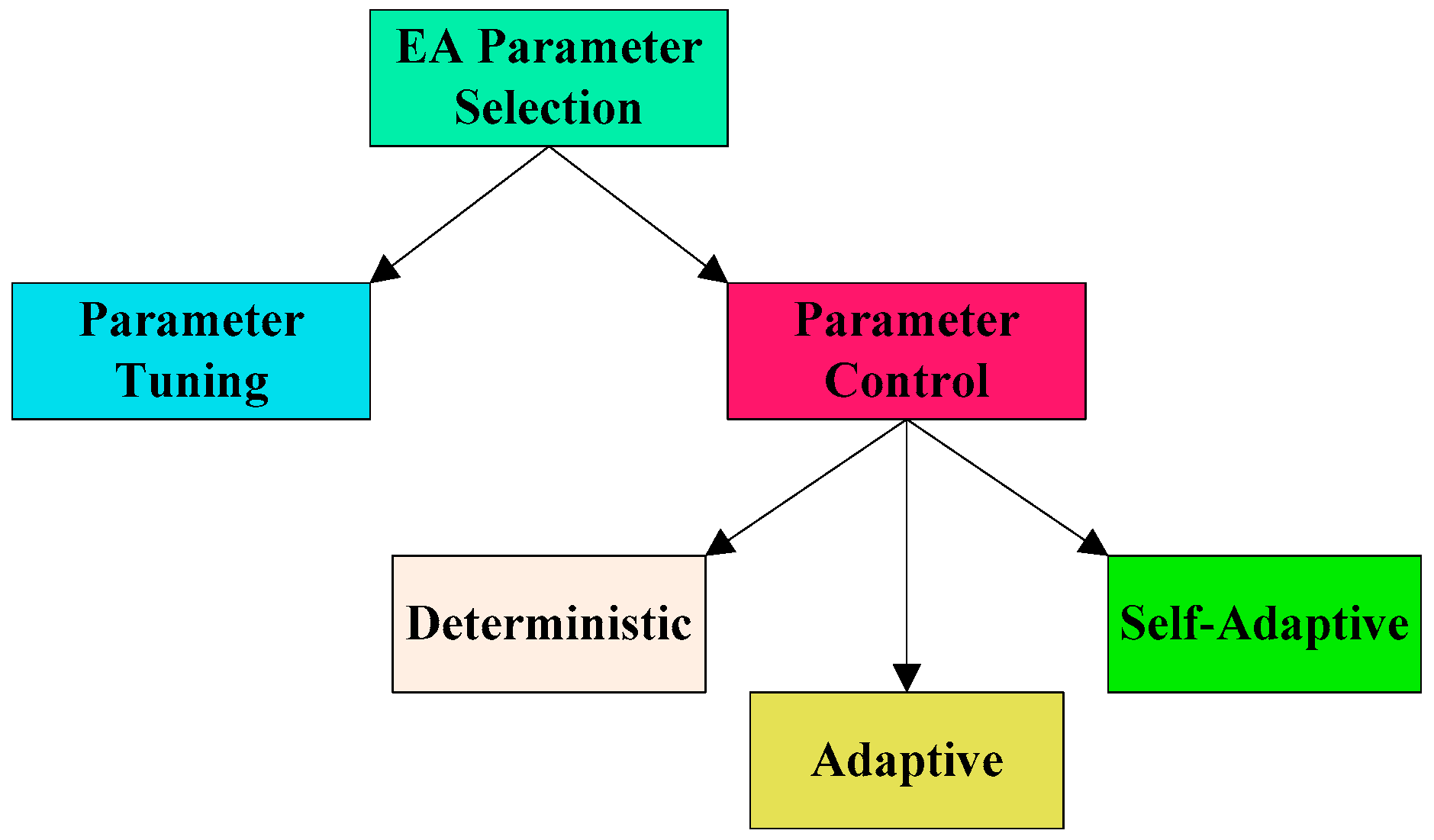
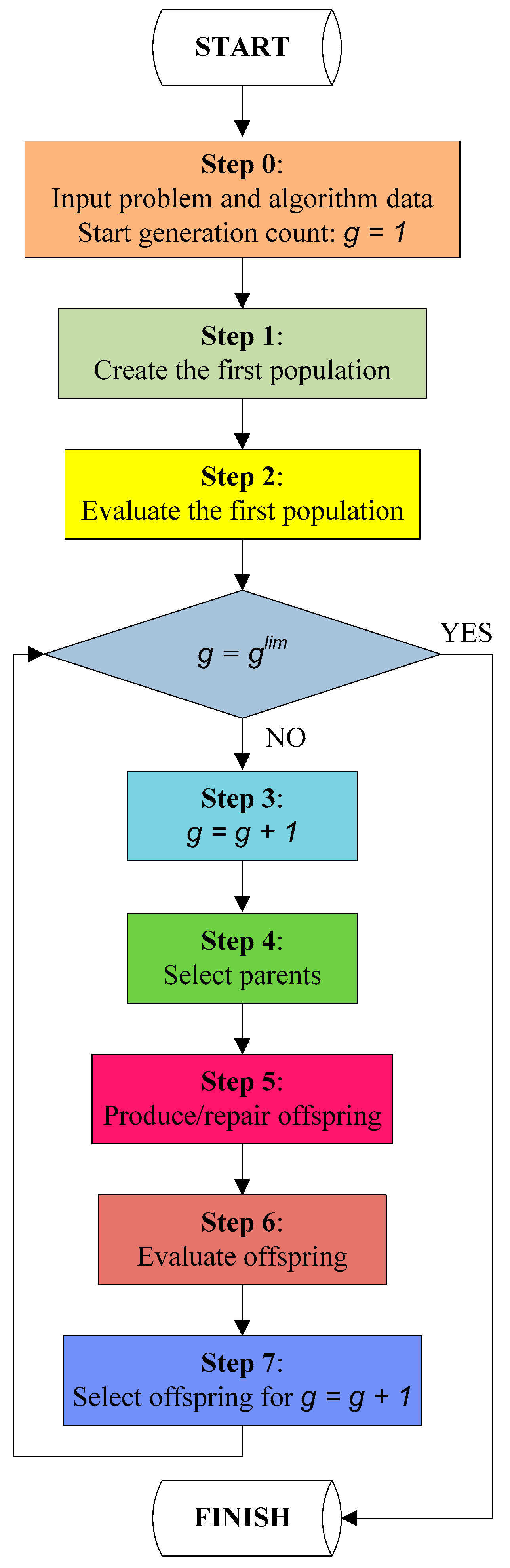
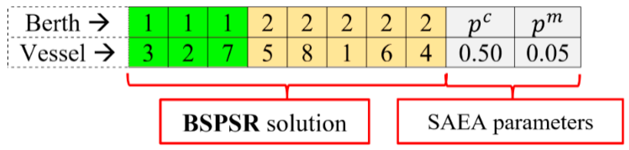
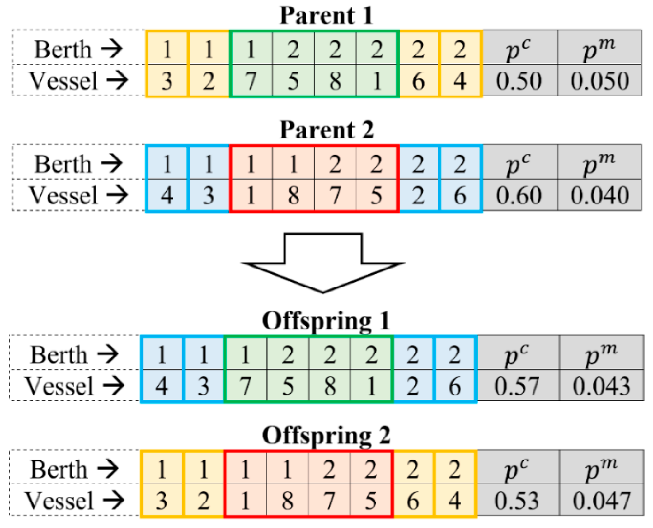
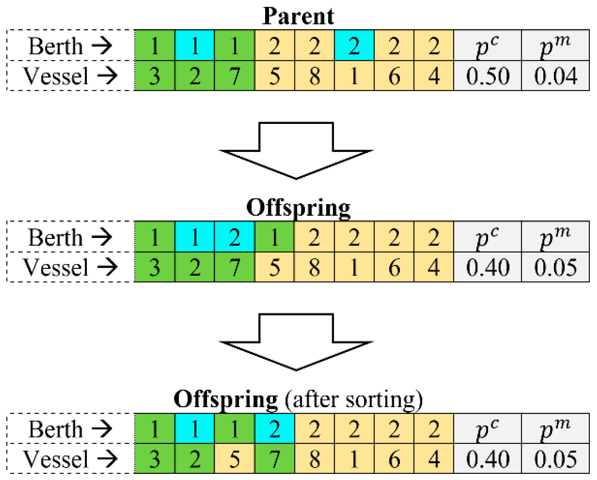
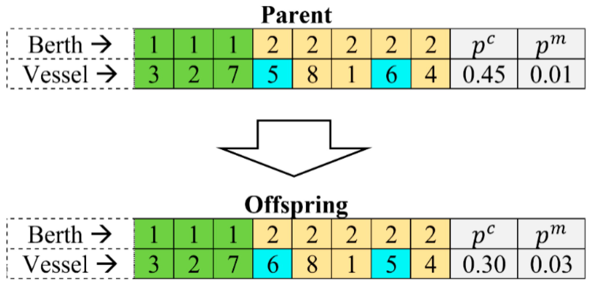
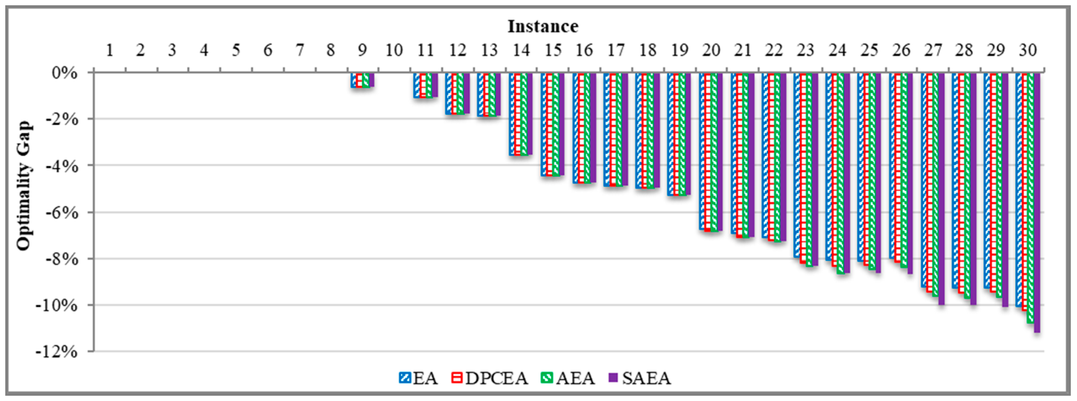
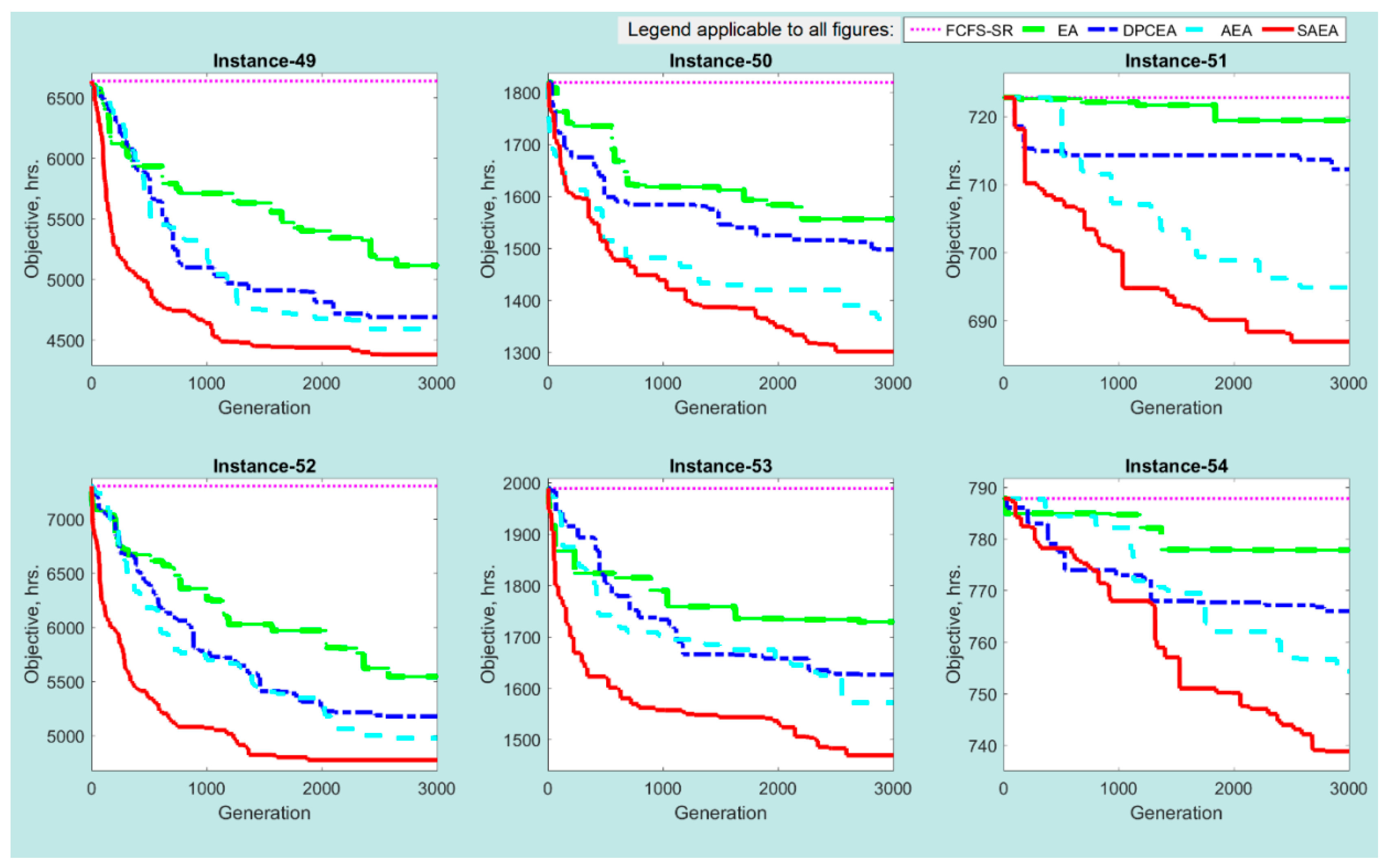
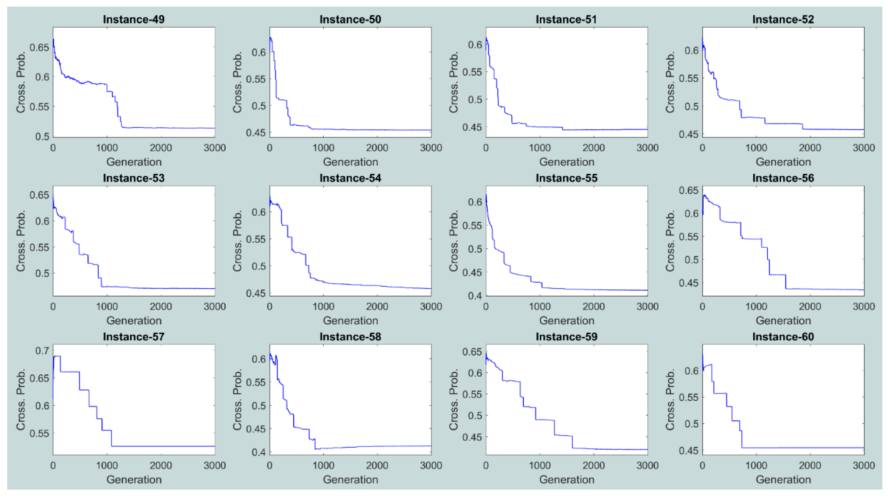
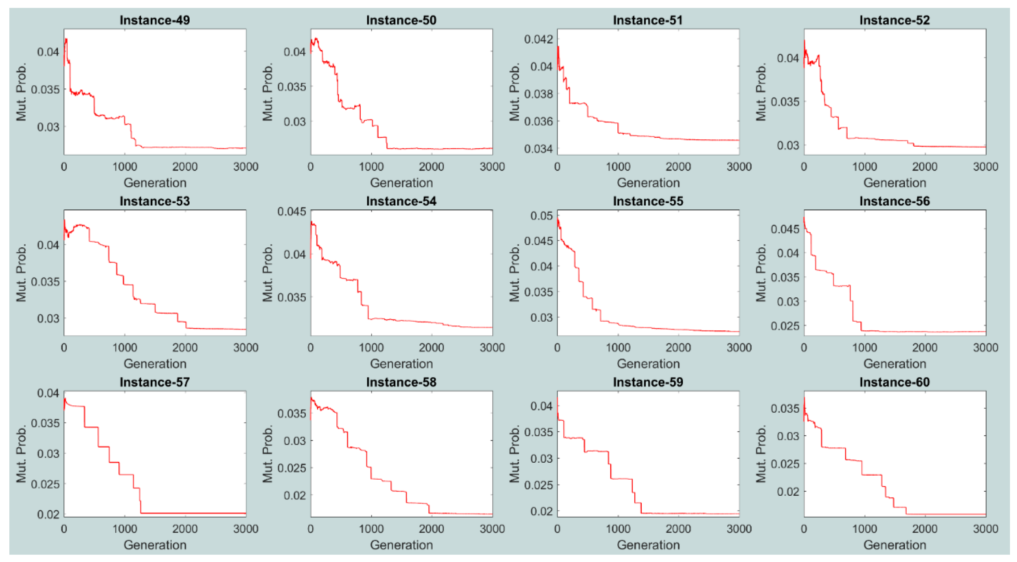
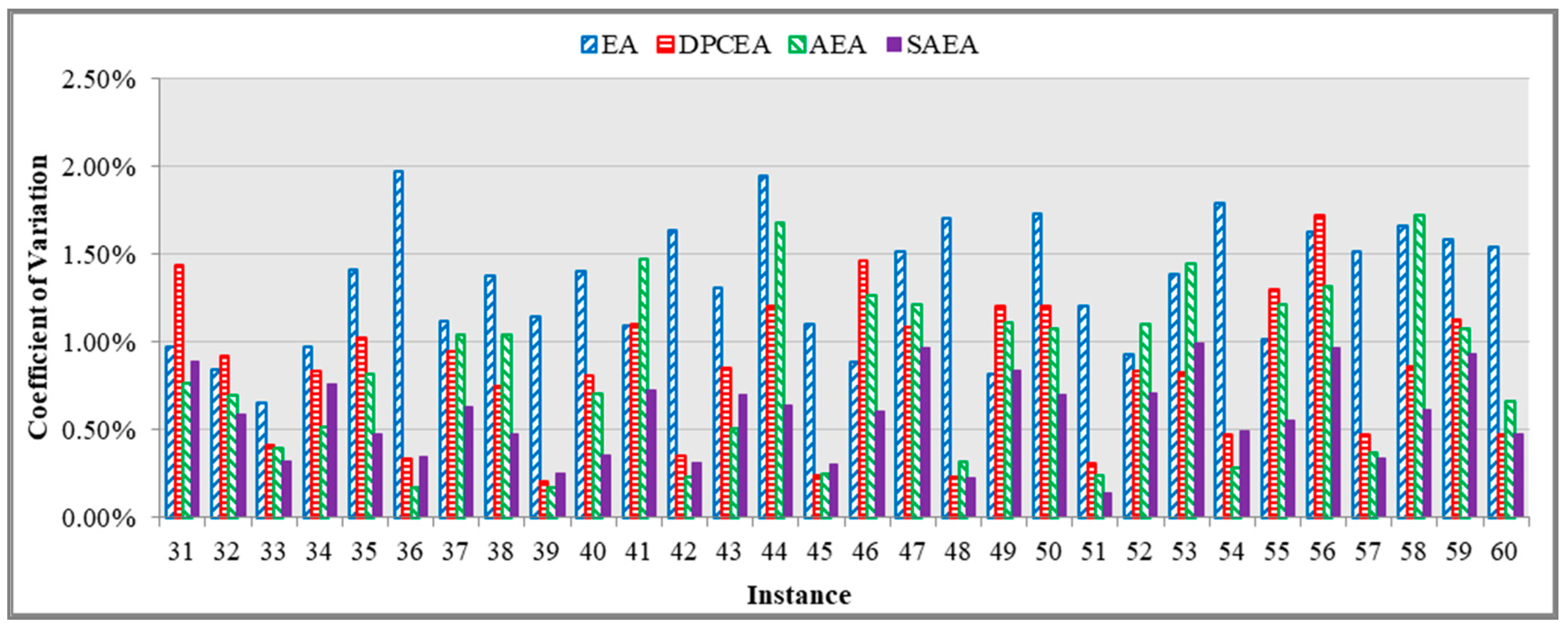
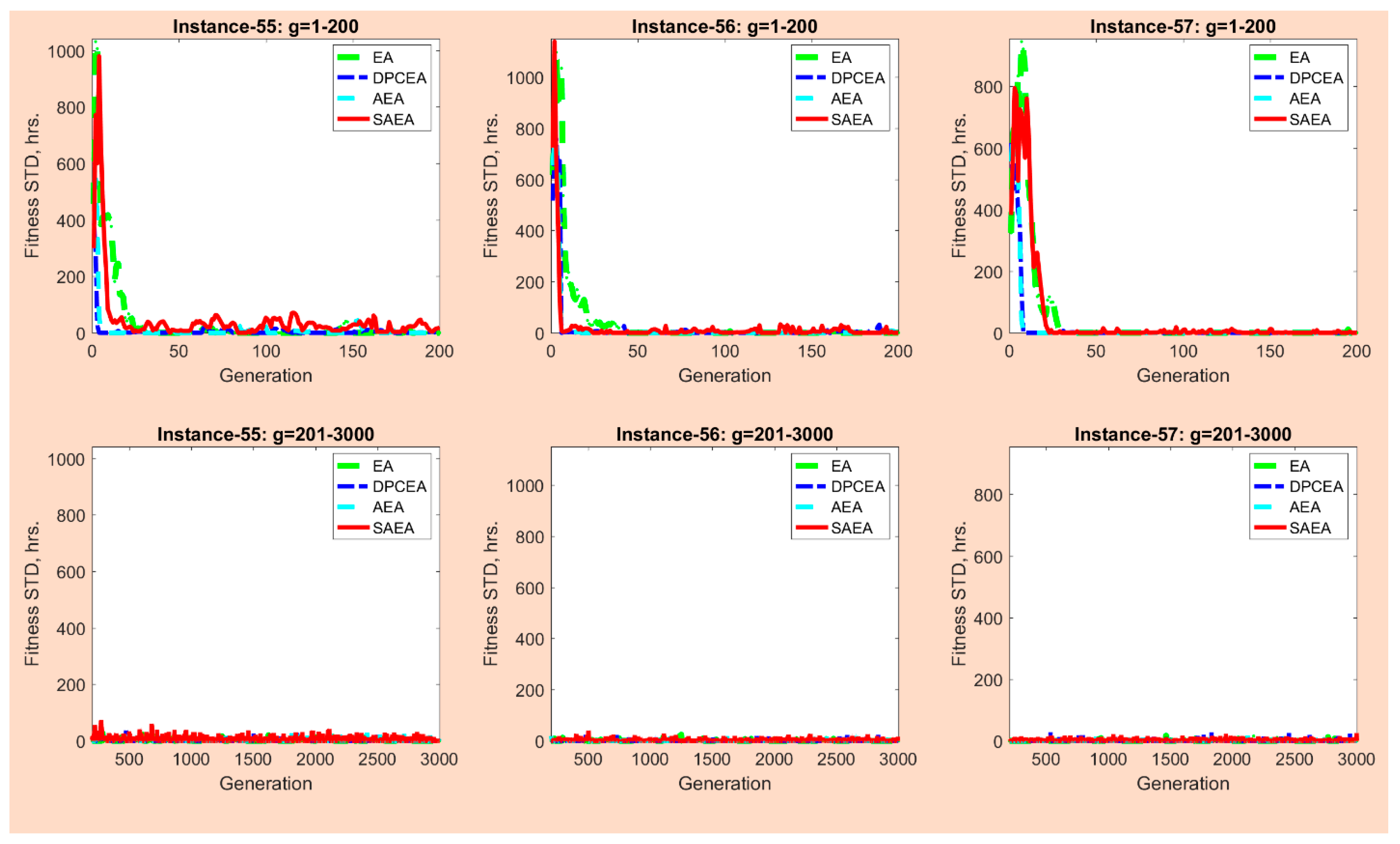
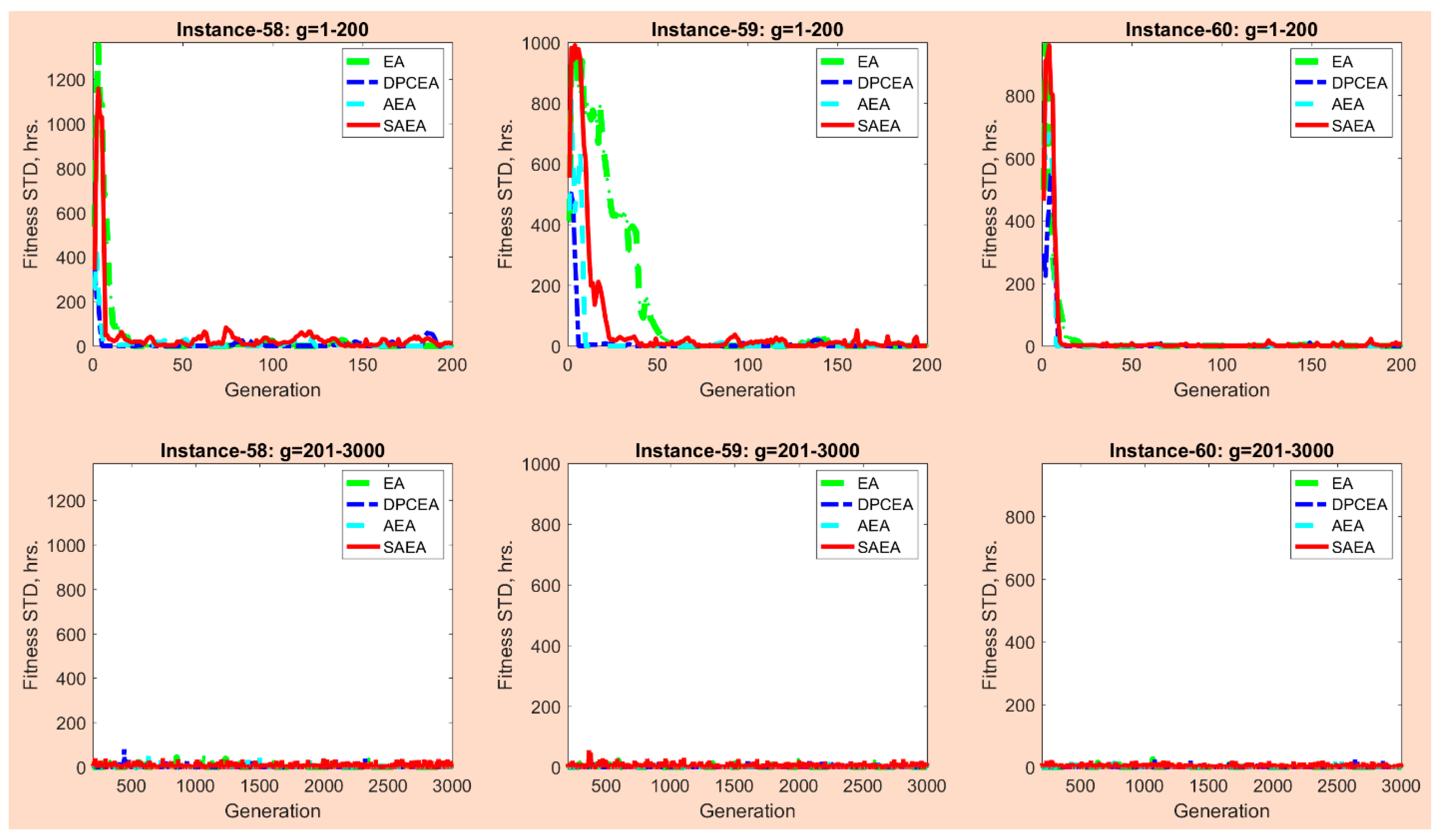
Table 1.
Description of the mathematical model components.
| Model Component | Description | |
|---|---|---|
| Type | Nomenclature | |
| Sets | set of arriving vessels (vessels) | |
| set of available berthing positions (berthing positions) | ||
| set of vessel service orders (service orders) | ||
| Decision Variables | =1 if vessel is assigned to berthing position in service order (=0 otherwise) | |
| Auxiliary Variables | idle time of berthing position between the start service time of vessel and a preceding vessel served as vessel (h) | |
| start service time of vessel (h) | ||
| finish service time of vessel (h) | ||
| waiting time of vessel (h) | ||
| late departure time of vessel (h) | ||
| Parameters | number of arriving vessels (vessels) | |
| number of available berthing positions (berthing positions) | ||
| number of vessel service orders (service orders) | ||
| time when berthing position becomes available in the planning horizon for the first time (h) | ||
| arrival time of vessel at the MCT (h) | ||
| handling time of vessel at berthing position (h) | ||
| negotiated departure time of vessel (h) | ||
| length of vessel (ft.) | ||
| length of berthing position (ft.) | ||
| horizontal clearance requirement for vessel (ft.) | ||
| draft of vessel (ft.) | ||
| depth of berthing position (ft.) | ||
| vertical clearance requirement for vessel (ft.) | ||
| weight of vessel (value ranging from 0.10 to 1.00) | ||
| large positive number | ||
Table 2.
Adopted parameter values.
| Parameter | Selected Value |
|---|---|
| Number of arriving vessels: (vessels) | Varies depending on the problem instance |
| Number of available berthing positions: (berthing positions) | Varies depending on the problem instance |
| Number of vessel service orders: (service orders) | (assuming that all vessels can be assigned to a berth) |
| Time when berthing position becomes available in the planning horizon at the first time: (h) | |
| Arrival time of vessel at the MCT: (h) | |
| Average vessel inter-arrival time: (h) | |
| Handling time of vessel at “preferred berthing position”: (h) | |
| “Preferred berthing position” for vessel : (berthing position) | |
| Handling time of vessel at berthing position : (h) | |
| Negotiated departure time of vessel : (h) | |
| Length of vessel : (ft.) | |
| Length of berthing position : (ft.) | |
| Horizontal clearance requirement for vessel : (ft.) | |
| Draft of vessel : (ft.) | |
| Depth of berthing position : (ft.) | |
| Vertical clearance requirement for vessel : (ft.) | |
| Weight of vessel : | |
| Large positive number: |
Table 3.
The parameter tuning analysis results for the developed solution algorithms.
| Algorithm | Parameter | Candidate Values | Best Value | Algorithm | Parameter | Candidate Values | Best Value |
|---|---|---|---|---|---|---|---|
| SAEA | Population size () | [40; 50; 60] | 60 | DPCEA | [0.80, 0.30; 0.90, 0.40; 0.30, 0.80] | [0.80, 0.30] | |
| SAEA | [50; 75; 100] | 100 | DPCEA | [0.06, 0.01; 0.07, 0.02; 0.01,0.06] | [0.06, 0.01] | ||
| SAEA | [1000; 2000; 3000] | 3000 | DPCEA | [10; 15; 20] | 10 | ||
| AEA | Population size () | [40; 50; 60] | 60 | DPCEA | [50; 75; 100] | 100 | |
| AEA | [0.80 ÷ 0.30; 0.90 ÷ 0.40; 0.30 ÷ 0.80] 1 | [0.80 ÷ 0.30] | DPCEA | [1000; 2000; 3000] | 3000 | ||
| AEA | [0.06 ÷ 0.01; 0.07 ÷ 0.02; 0.01 ÷ 0.06] 2 | [0.06 ÷ 0.01] | EA | Population size () | [40; 50; 60] | 60 | |
| AEA | [100; 200; 300] | 300 | EA | [0.30; 0.50; 0.80] | 0.80 | ||
| AEA | [50; 75; 100] | 100 | EA | [0.01; 0.04; 0.06] | 0.06 | ||
| AEA | [1000; 2000; 3000] | 3000 | EA | [50; 75; 100] | 100 | ||
| DPCEA | Population size () | [40; 50; 60] | 60 | EA | [1000; 2000; 3000] | 3000 |
Notes: 1—the crossover probability values were changed with an increment of 0.10 within the AEA algorithm; 2—the mutation probability values were changed with an increment of 0.01 within the AEA algorithm.
Table 4.
Comparison of the developed solution algorithms against CPLEX.
| Instance | Number of Vessels | Number of Berths | CPLEX | EA | DPCEA | AEA | SAEA | |||||
|---|---|---|---|---|---|---|---|---|---|---|---|---|
| Objective, h | CPU, s | Objective, h | CPU, s | Objective, h | CPU, s | Objective, h | CPU, s | Objective, h | CPU, s | |||
| 1 | 5 | 2 | 57.381 | 1.70 | 57.381 | 6.63 | 57.381 | 9.38 | 57.381 | 10.85 | 57.381 | 11.42 |
| 2 | 5 | 3 | 42.203 | 4.52 | 42.203 | 6.63 | 42.203 | 9.14 | 42.203 | 10.76 | 42.203 | 11.46 |
| 3 | 5 | 4 | 35.923 | 5.92 | 35.923 | 6.62 | 35.923 | 9.17 | 35.923 | 10.62 | 35.923 | 11.08 |
| 4 | 6 | 2 | 102.008 | 13.82 | 102.008 | 6.91 | 102.008 | 9.59 | 102.008 | 11.34 | 102.008 | 11.77 |
| 5 | 6 | 3 | 72.644 | 153.00 | 72.644 | 6.88 | 72.644 | 9.61 | 72.644 | 11.32 | 72.644 | 11.96 |
| 6 | 6 | 4 | 58.514 | 421.02 | 58.514 | 6.88 | 58.514 | 9.59 | 58.514 | 11.21 | 58.514 | 11.67 |
| 7 | 7 | 2 | 120.643 | 187.49 | 120.643 | 7.15 | 120.643 | 10.00 | 120.643 | 11.87 | 120.643 | 12.53 |
| 8 | 7 | 3 | 86.639 | 3344.27 | 86.639 | 7.13 | 86.639 | 10.01 | 86.639 | 11.64 | 86.639 | 12.03 |
| 9 | 7 | 4 | 67.686 | 7203.40 | 67.261 | 7.08 | 67.261 | 10.06 | 67.261 | 11.43 | 67.261 | 12.18 |
| 10 | 8 | 2 | 173.560 | 3878.79 | 173.560 | 7.48 | 173.560 | 10.40 | 173.560 | 12.32 | 173.560 | 13.07 |
| 11 | 8 | 3 | 116.613 | 7207.12 | 115.379 | 7.39 | 115.379 | 10.41 | 115.379 | 12.09 | 115.379 | 12.83 |
| 12 | 8 | 4 | 87.940 | 7206.69 | 86.402 | 7.36 | 86.402 | 10.40 | 86.402 | 11.97 | 86.402 | 12.69 |
| 13 | 9 | 2 | 207.567 | 7207.17 | 203.697 | 7.68 | 203.697 | 10.83 | 203.697 | 12.79 | 203.697 | 13.41 |
| 14 | 9 | 3 | 138.080 | 7205.43 | 133.192 | 7.68 | 133.192 | 10.84 | 133.192 | 12.40 | 133.192 | 13.17 |
| 15 | 9 | 4 | 100.693 | 7205.23 | 96.255 | 7.68 | 96.255 | 10.82 | 96.255 | 12.41 | 96.255 | 12.94 |
| 16 | 10 | 2 | 260.008 | 7206.87 | 247.721 | 8.01 | 247.721 | 11.22 | 247.721 | 13.28 | 247.721 | 13.77 |
| 17 | 10 | 3 | 168.606 | 7204.10 | 160.394 | 7.97 | 160.394 | 11.23 | 160.394 | 12.96 | 160.394 | 13.62 |
| 18 | 10 | 4 | 121.324 | 7204.73 | 115.294 | 8.01 | 115.294 | 11.20 | 115.294 | 12.89 | 115.294 | 13.60 |
| 19 | 11 | 2 | 351.252 | 7204.96 | 332.783 | 8.30 | 332.783 | 11.63 | 332.783 | 14.03 | 332.783 | 14.64 |
| 20 | 11 | 3 | 234.583 | 7203.95 | 218.844 | 8.25 | 218.644 | 11.64 | 218.644 | 13.43 | 218.644 | 14.49 |
| 21 | 11 | 4 | 161.140 | 7203.51 | 149.983 | 8.27 | 149.703 | 11.77 | 149.703 | 13.25 | 149.703 | 13.92 |
| 22 | 12 | 2 | 458.371 | 7202.79 | 426.017 | 8.54 | 425.270 | 12.06 | 425.126 | 13.76 | 425.126 | 14.68 |
| 23 | 12 | 3 | 290.278 | 7205.62 | 267.282 | 8.56 | 266.475 | 12.13 | 266.188 | 13.24 | 266.188 | 14.41 |
| 24 | 12 | 4 | 204.840 | 7202.84 | 188.303 | 8.60 | 187.840 | 12.14 | 187.188 | 13.20 | 187.188 | 14.45 |
| 25 | 13 | 2 | 559.488 | 7202.04 | 514.104 | 8.90 | 513.240 | 12.49 | 512.251 | 14.07 | 511.228 | 15.86 |
| 26 | 13 | 3 | 336.885 | 7202.05 | 310.100 | 8.84 | 309.459 | 12.48 | 308.718 | 13.71 | 307.714 | 15.13 |
| 27 | 13 | 4 | 235.101 | 7202.10 | 213.489 | 8.86 | 212.951 | 12.54 | 212.496 | 13.75 | 211.555 | 14.93 |
| 28 | 14 | 2 | 669.643 | 7201.96 | 607.726 | 9.21 | 606.304 | 12.94 | 604.744 | 14.63 | 602.522 | 16.06 |
| 29 | 14 | 3 | 431.216 | 7201.61 | 391.360 | 9.11 | 390.528 | 12.93 | 389.541 | 14.13 | 387.749 | 15.57 |
| 30 | 14 | 4 | 294.092 | 7201.42 | 264.557 | 9.20 | 263.990 | 12.95 | 262.488 | 14.19 | 261.114 | 15.48 |
| Average: | 208.164 | 5309.87 | 195.322 | 7.86 | 195.077 | 11.05 | 194.833 | 12.65 | 194.554 | 13.49 | ||
Table 5.
The objective function and computational time values for the developed solution algorithms and large size problem instances.
Table 5.
The objective function and computational time values for the developed solution algorithms and large size problem instances.
| Instance | Number of Vessels | Number of Berths | EA | DPCEA | AEA | SAEA | ||||
|---|---|---|---|---|---|---|---|---|---|---|
| Objective, h | CPU, s | Objective, h | CPU, s | Objective, h | CPU, s | Objective, h | CPU, s | |||
| 31 | 55 | 4 | 2377.761 | 22.21 | 2258.330 | 31.40 | 2211.918 | 33.54 | 2164.059 | 39.32 |
| 32 | 55 | 6 | 899.983 | 21.67 | 854.218 | 31.37 | 825.216 | 33.72 | 788.960 | 39.02 |
| 33 | 55 | 8 | 455.552 | 21.72 | 447.148 | 31.50 | 442.022 | 34.46 | 437.173 | 39.17 |
| 34 | 60 | 4 | 2800.193 | 23.16 | 2631.300 | 33.63 | 2591.382 | 35.80 | 2525.668 | 40.99 |
| 35 | 60 | 6 | 1011.343 | 22.40 | 975.456 | 33.83 | 924.069 | 35.91 | 886.146 | 41.64 |
| 36 | 60 | 8 | 496.764 | 22.38 | 491.083 | 34.21 | 484.617 | 37.24 | 479.352 | 42.03 |
| 37 | 65 | 4 | 3205.971 | 24.41 | 3019.285 | 36.10 | 2988.301 | 38.02 | 2896.303 | 44.05 |
| 38 | 65 | 6 | 1119.997 | 24.43 | 1065.933 | 35.95 | 1030.017 | 39.85 | 985.366 | 43.56 |
| 39 | 65 | 8 | 545.141 | 24.46 | 538.879 | 35.90 | 532.089 | 41.19 | 525.534 | 43.78 |
| 40 | 70 | 4 | 3544.719 | 25.36 | 3357.861 | 37.94 | 3253.702 | 42.02 | 3168.028 | 47.18 |
| 41 | 70 | 6 | 1213.662 | 25.45 | 1148.926 | 38.04 | 1092.158 | 42.38 | 1045.119 | 46.54 |
| 42 | 70 | 8 | 572.387 | 25.60 | 568.528 | 38.21 | 560.240 | 43.33 | 556.178 | 47.27 |
| 43 | 75 | 4 | 4034.567 | 27.17 | 3740.517 | 40.11 | 3681.803 | 43.28 | 3544.645 | 49.66 |
| 44 | 75 | 6 | 1324.011 | 27.01 | 1248.610 | 40.16 | 1197.125 | 43.64 | 1113.764 | 49.39 |
| 45 | 75 | 8 | 617.365 | 26.94 | 611.086 | 40.63 | 602.913 | 45.16 | 597.957 | 49.78 |
| 46 | 80 | 4 | 4472.340 | 28.16 | 4153.364 | 42.18 | 4088.902 | 45.33 | 3902.842 | 51.80 |
| 47 | 80 | 6 | 1420.608 | 28.10 | 1343.371 | 42.21 | 1271.579 | 45.98 | 1193.858 | 52.39 |
| 48 | 80 | 8 | 654.161 | 28.19 | 646.792 | 42.37 | 638.393 | 47.51 | 630.520 | 52.22 |
| 49 | 85 | 4 | 5071.830 | 29.82 | 4695.141 | 44.42 | 4591.242 | 47.78 | 4396.188 | 54.48 |
| 50 | 85 | 6 | 1544.441 | 29.88 | 1469.839 | 44.64 | 1399.679 | 47.67 | 1310.340 | 56.30 |
| 51 | 85 | 8 | 717.262 | 30.00 | 706.896 | 44.89 | 695.856 | 48.94 | 687.353 | 55.98 |
| 52 | 90 | 4 | 5566.083 | 31.30 | 5197.091 | 46.69 | 5052.644 | 50.32 | 4791.672 | 57.59 |
| 53 | 90 | 6 | 1718.440 | 31.41 | 1616.241 | 46.72 | 1557.377 | 50.94 | 1443.065 | 58.82 |
| 54 | 90 | 8 | 777.947 | 31.48 | 767.060 | 46.99 | 751.242 | 53.37 | 738.916 | 59.11 |
| 55 | 95 | 4 | 6260.245 | 32.81 | 5745.434 | 48.82 | 5625.241 | 52.88 | 5252.036 | 61.11 |
| 56 | 95 | 6 | 1921.365 | 32.82 | 1815.067 | 48.84 | 1747.256 | 53.96 | 1618.356 | 60.67 |
| 57 | 95 | 8 | 851.889 | 32.84 | 840.441 | 49.14 | 821.427 | 56.16 | 803.427 | 61.73 |
| 58 | 100 | 4 | 7028.538 | 34.00 | 6519.833 | 51.18 | 6361.047 | 55.59 | 5959.020 | 64.96 |
| 59 | 100 | 6 | 2144.635 | 34.16 | 2024.188 | 51.24 | 1952.334 | 55.57 | 1805.210 | 63.55 |
| 60 | 100 | 8 | 939.400 | 34.30 | 917.367 | 51.39 | 901.137 | 56.36 | 874.526 | 63.67 |
| Average: | 2176.953 | 27.79 | 2047.176 | 41.36 | 1995.764 | 45.26 | 1904.053 | 51.26 | ||
Table 6.
The one-way ANOVA analysis results.
| Instance | Number of Vessels | Number of Berths | SAEA vs. EA | SAEA vs. DPCEA | SAEA vs. AEA | |||
|---|---|---|---|---|---|---|---|---|
| F-Statistic | p-Value | F-Statistic | P-Value | F-Statistic | p-Value | |||
| 31 | 55 | 4 | 87.333 | 2.51 × 10⁻⁸ | 15.560 | 9.50 × 10⁻⁴ | 8.707 | 8.55 × 10⁻³ |
| 32 | 55 | 6 | 185.969 | 6.28 × 10⁻¹¹ | 127.441 | 1.34 × 10⁻⁹ | 59.595 | 4.06 × 10⁻⁷ |
| 33 | 55 | 8 | 200.004 | 3.44 × 10⁻¹¹ | 45.171 | 2.66 × 10⁻⁶ | 11.298 | 3.48 × 10⁻³ |
| 34 | 60 | 4 | 111.444 | 3.86 × 10⁻⁹ | 32.717 | 2.01 × 10⁻⁵ | 19.747 | 3.14 × 10⁻⁴ |
| 35 | 60 | 6 | 88.500 | 2.27 × 10⁻⁸ | 168.485 | 1.41 × 10⁻¹⁰ | 47.567 | 1.89 × 10⁻⁶ |
| 36 | 60 | 8 | 117.671 | 2.52 × 10⁻⁹ | 61.920 | 3.10 × 10⁻⁷ | 19.533 | 3.31 × 10⁻⁴ |
| 37 | 65 | 4 | 72.669 | 9.80 × 10⁻⁸ | 45.253 | 2.63 × 10⁻⁶ | 16.209 | 7.93 × 10⁻⁴ |
| 38 | 65 | 6 | 128.470 | 1.26 × 10⁻⁹ | 186.894 | 6.02 × 10⁻¹¹ | 36.215 | 1.09 × 10⁻⁵ |
| 39 | 65 | 8 | 273.436 | 2.50 × 10⁻¹² | 142.323 | 5.55 × 10⁻¹⁰ | 39.893 | 5.94 × 10⁻⁶ |
| 40 | 70 | 4 | 199.458 | 3.52 × 10⁻¹¹ | 102.829 | 7.20 × 10⁻⁹ | 27.968 | 4.99 × 10⁻⁵ |
| 41 | 70 | 6 | 196.358 | 4.00 × 10⁻¹¹ | 122.740 | 1.81 × 10⁻⁹ | 17.452 | 5.66 × 10⁻⁴ |
| 42 | 70 | 8 | 162.601 | 1.89 × 10⁻¹⁰ | 54.086 | 7.95 × 10⁻⁷ | 8.545 | 9.08 × 10⁻³ |
| 43 | 75 | 4 | 178.851 | 8.65 × 10⁻¹¹ | 58.665 | 4.53 × 10⁻⁷ | 48.762 | 1.60 × 10⁻⁶ |
| 44 | 75 | 6 | 532.901 | 7.99 × 10⁻¹⁵ | 162.142 | 1.93 × 10⁻¹⁰ | 38.115 | 7.91 × 10⁻⁶ |
| 45 | 75 | 8 | 149.522 | 3.73 × 10⁻¹⁰ | 78.246 | 5.69 × 10⁻⁸ | 10.726 | 4.21 × 10⁻³ |
| 46 | 80 | 4 | 250.318 | 5.27 × 10⁻¹² | 41.776 | 4.42 × 10⁻⁶ | 26.552 | 6.68 × 10⁻⁵ |
| 47 | 80 | 6 | 126.959 | 1.38 × 10⁻⁹ | 160.559 | 2.09 × 10⁻¹⁰ | 40.397 | 5.48 × 10⁻⁶ |
| 48 | 80 | 8 | 291.768 | 1.44 × 10⁻¹² | 155.394 | 2.73 × 10⁻¹⁰ | 24.430 | 1.05 × 10⁻⁴ |
| 49 | 85 | 4 | 113.627 | 3.31 × 10⁻⁹ | 56.399 | 5.96 × 10⁻⁷ | 23.833 | 1.20 × 10⁻⁴ |
| 50 | 85 | 6 | 208.291 | 2.45 × 10⁻¹¹ | 158.601 | 2.31 × 10⁻¹⁰ | 63.882 | 2.48 × 10⁻⁷ |
| 51 | 85 | 8 | 333.197 | 4.63 × 10⁻¹³ | 160.421 | 2.11 × 10⁻¹⁰ | 45.943 | 2.38 × 10⁻⁶ |
| 52 | 90 | 4 | 149.621 | 3.71 × 10⁻¹⁰ | 141.627 | 5.77 × 10⁻¹⁰ | 39.692 | 6.13 × 10⁻⁶ |
| 53 | 90 | 6 | 279.916 | 2.05 × 10⁻¹² | 193.527 | 4.52 × 10⁻¹¹ | 45.672 | 2.48 × 10⁻⁶ |
| 54 | 90 | 8 | 116.989 | 2.64 × 10⁻⁹ | 75.017 | 7.77 × 10⁻⁸ | 21.291 | 2.15 × 10⁻⁴ |
| 55 | 95 | 4 | 245.548 | 6.19 × 10⁻¹² | 130.574 | 1.10 × 10⁻⁹ | 62.830 | 2.79 × 10⁻⁷ |
| 56 | 95 | 6 | 593.439 | 3.12 × 10⁻¹⁵ | 78.704 | 5.45 × 10⁻⁸ | 53.649 | 8.41 × 10⁻⁷ |
| 57 | 95 | 8 | 294.788 | 1.32 × 10⁻¹² | 145.754 | 4.58 × 10⁻¹⁰ | 47.897 | 1.81 × 10⁻⁶ |
| 58 | 100 | 4 | 185.464 | 6.42 × 10⁻¹¹ | 174.531 | 1.06 × 10⁻¹⁰ | 30.213 | 3.21 × 10⁻⁵ |
| 59 | 100 | 6 | 293.450 | 1.37 × 10⁻¹² | 148.309 | 3.98 × 10⁻¹⁰ | 74.222 | 8.40 × 10⁻⁸ |
| 60 | 100 | 8 | 136.192 | 7.89 × 10⁻¹⁰ | 123.778 | 1.69 × 10⁻⁹ | 32.833 | 1.97 × 10⁻⁵ |
| Average: | 210.158 | 5.43 × 10⁻⁹ | 111.648 | 3.27 × 10⁻⁵ | 34.789 | 9.33 × 10⁻⁴ | ||
Table 7.
The convergence rate values for the developed solution algorithms and large size problem instances.
Table 7.
The convergence rate values for the developed solution algorithms and large size problem instances.
| Instance | Number of Vessels | Number of Berths | EA | DPCEA | AEA | SAEA | ||||
|---|---|---|---|---|---|---|---|---|---|---|
| 31 | 55 | 4 | 0.904 | 0.050 | 0.863 | 0.086 | 0.959 | 0.030 | 0.837 | 0.159 |
| 32 | 55 | 6 | 0.853 | 0.150 | 0.869 | 0.117 | 0.959 | 0.039 | 0.873 | 0.115 |
| 33 | 55 | 8 | 0.941 | 0.043 | 0.838 | 0.130 | 0.943 | 0.032 | 0.897 | 0.119 |
| 34 | 60 | 4 | 0.948 | 0.046 | 0.922 | 0.082 | 0.939 | 0.048 | 0.921 | 0.079 |
| 35 | 60 | 6 | 0.912 | 0.073 | 0.908 | 0.072 | 0.933 | 0.073 | 0.911 | 0.077 |
| 36 | 60 | 8 | 0.804 | 0.162 | 0.784 | 0.215 | 0.955 | 0.052 | 0.948 | 0.041 |
| 37 | 65 | 4 | 0.923 | 0.076 | 0.841 | 0.180 | 0.952 | 0.065 | 0.822 | 0.149 |
| 38 | 65 | 6 | 0.845 | 0.103 | 0.906 | 0.077 | 0.941 | 0.057 | 0.906 | 0.110 |
| 39 | 65 | 8 | 0.659 | 0.269 | 0.848 | 0.125 | 0.966 | 0.034 | 0.946 | 0.033 |
| 40 | 70 | 4 | 0.914 | 0.082 | 0.967 | 0.028 | 0.950 | 0.037 | 0.885 | 0.157 |
| 41 | 70 | 6 | 0.867 | 0.113 | 0.922 | 0.051 | 0.944 | 0.019 | 0.922 | 0.068 |
| 42 | 70 | 8 | 0.668 | 0.277 | 0.889 | 0.102 | 0.959 | 0.044 | 0.931 | 0.076 |
| 43 | 75 | 4 | 0.885 | 0.135 | 0.907 | 0.066 | 0.961 | 0.032 | 0.877 | 0.135 |
| 44 | 75 | 6 | 0.871 | 0.104 | 0.934 | 0.091 | 0.956 | 0.041 | 0.873 | 0.134 |
| 45 | 75 | 8 | 0.828 | 0.172 | 0.897 | 0.075 | 0.955 | 0.019 | 0.915 | 0.085 |
| 46 | 80 | 4 | 0.886 | 0.102 | 0.914 | 0.058 | 0.954 | 0.052 | 0.948 | 0.046 |
| 47 | 80 | 6 | 0.812 | 0.178 | 0.933 | 0.057 | 0.953 | 0.042 | 0.912 | 0.073 |
| 48 | 80 | 8 | 0.771 | 0.206 | 0.885 | 0.071 | 0.965 | 0.032 | 0.957 | 0.043 |
| 49 | 85 | 4 | 0.969 | 0.037 | 0.921 | 0.072 | 0.953 | 0.036 | 0.898 | 0.103 |
| 50 | 85 | 6 | 0.878 | 0.109 | 0.921 | 0.059 | 0.956 | 0.039 | 0.939 | 0.093 |
| 51 | 85 | 8 | 0.799 | 0.331 | 0.839 | 0.132 | 0.947 | 0.047 | 0.950 | 0.038 |
| 52 | 90 | 4 | 0.945 | 0.031 | 0.890 | 0.102 | 0.937 | 0.047 | 0.854 | 0.127 |
| 53 | 90 | 6 | 0.912 | 0.042 | 0.852 | 0.095 | 0.956 | 0.044 | 0.916 | 0.059 |
| 54 | 90 | 8 | 0.775 | 0.231 | 0.809 | 0.195 | 0.969 | 0.027 | 0.974 | 0.021 |
| 55 | 95 | 4 | 0.951 | 0.031 | 0.959 | 0.053 | 0.950 | 0.049 | 0.950 | 0.048 |
| 56 | 95 | 6 | 0.878 | 0.101 | 0.931 | 0.072 | 0.965 | 0.043 | 0.932 | 0.090 |
| 57 | 95 | 8 | 0.824 | 0.167 | 0.803 | 0.140 | 0.969 | 0.023 | 0.949 | 0.074 |
| 58 | 100 | 4 | 0.933 | 0.063 | 0.917 | 0.068 | 0.970 | 0.030 | 0.916 | 0.087 |
| 59 | 100 | 6 | 0.907 | 0.093 | 0.926 | 0.061 | 0.946 | 0.034 | 0.952 | 0.049 |
| 60 | 100 | 8 | 0.744 | 0.127 | 0.880 | 0.118 | 0.968 | 0.025 | 0.958 | 0.035 |
| Average: | 0.860 | 0.123 | 0.889 | 0.095 | 0.954 | 0.040 | 0.916 | 0.084 | ||
© 2018 by the authors. Licensee MDPI, Basel, Switzerland. This article is an open access article distributed under the terms and conditions of the Creative Commons Attribution (CC BY) license (http://creativecommons.org/licenses/by/4.0/).
Share and Cite
MDPI and ACS Style
Dulebenets, M.A.; Kavoosi, M.; Abioye, O.; Pasha, J. A Self-Adaptive Evolutionary Algorithm for the Berth Scheduling Problem: Towards Efficient Parameter Control. Algorithms 2018, 11, 100. https://doi.org/10.3390/a11070100
AMA Style
Dulebenets MA, Kavoosi M, Abioye O, Pasha J. A Self-Adaptive Evolutionary Algorithm for the Berth Scheduling Problem: Towards Efficient Parameter Control. Algorithms. 2018; 11(7):100. https://doi.org/10.3390/a11070100
Chicago/Turabian StyleDulebenets, Maxim A., Masoud Kavoosi, Olumide Abioye, and Junayed Pasha. 2018. "A Self-Adaptive Evolutionary Algorithm for the Berth Scheduling Problem: Towards Efficient Parameter Control" Algorithms 11, no. 7: 100. https://doi.org/10.3390/a11070100
Note that from the first issue of 2016, this journal uses article numbers instead of page numbers. See further details here.