Solutions to the Sub-Optimality and Stability Issues of Recursive Pole and Zero Distribution Algorithms for the Approximation of Fractional Order Models

IMS-UMR 5218 CNRS Laboratory, Bordeaux University, 33405 Talence CEDEX, France
Algorithms 2018, 11(7), 103; https://doi.org/10.3390/a11070103
Submission received: 31 May 2018
/
Revised: 26 June 2018
/
Accepted: 28 June 2018
/
Published: 12 July 2018
(This article belongs to the Special Issue Fractional Order Systems and Signals: Modelling, Identification and Control Applications)
Abstract
:This paper analyses algorithms currently found in the literature for the approximation of fractional order models and based on recursive pole and zero distributions. The analysis focuses on the sub-optimality of the approximations obtained and stability issues that may appear after approximation depending on the pole location of the initial fractional order model. Solutions are proposed to reduce this sub-optimality and to avoid stability issues.
1. Introduction
Fractional order models are generalizations of models described by differential equations or state space descriptions in which classical derivatives are replaced by fractional derivatives [1,2,3]. These models are now widely used to characterize the behavior of many systems in diverse areas. For example:
- -
- -
- -
- biology for modelling complex dynamics in biological tissues [9];
- -
- mechanics with the dynamical property of viscoelastic materials and for wave propagation problems in these materials [10];
- -
- acoustics where fractional differentiation is used to model visco-thermal losses in wind instruments [11];
- -
- robotics through environmental modeling [12];
- -
- electrical distribution networks [13];
- -
- modelling of explosive materials [14].
The main reason for the use of fractional order models is their ability to generate long memory behaviors (time power law relaxations) in the same way as the systems previously mentioned. However, this interesting property comes at the price of several defects that have important consequences in the field of dynamical system analysis:
- -
- -
- -
- -
This work looks at this approximation step. There are several methods in the literature that allow such an approximation. Among all these methods, a very well-known one because of its efficiency and the simple algorithm that it implements is based on the approximation of the fractional order differentiation or integration operator using a recursive (geometric) pole and zero distribution [21,22]. In this paper, this method is analyzed in terms of sub-optimality and a simple solution is proposed to improve the approximation accuracy. Some stability issues resulting from the approximation of a fractional model are also discussed. The results presented in this paper will contribute to obtaining more accurate and stable approximations of a fractional model, and above all will help the reader to understand that the geometric distribution of poles and zeros (also called “recursivity” in the literature) for the approximation of a fractional order integrator and differentiator is one among an infinity of other permitted distributions and cannot be interpreted as the physical reason for the observed long memory behaviors.
2. The Existing Algorithms Based on Pole and Zero Recursive (Geometric) Distribution
This section reviews the algorithms based on the recursive (geometric) pole and zero distribution found in the literature for the synthesis of a fractional order integrator or differentiator respectively described by the transfer functions:
2.1. Approximation of a Fractional Integrator and Differentiator by a Recursive (Geometric) Distribution of Pole and Zeros: A Graphical Approach
The demonstration of the approximation of a fractional order integrator operator frequency response is here done graphically. This method appeared for the very first time in the literature in the 1960s in two studies, apparently carried out independently by the respective authors [23,24]. Some years later, this demonstration was used for the analog implementation of fractional integrators [25]. Subsequent work by other authors also contributed to this synthesis method [26,27,28].
For real orders, to obtain an approximation of a fractional integration operator, a solution consists in limiting the frequency band on which the fractional behavior is required. This first leads to the approximation:
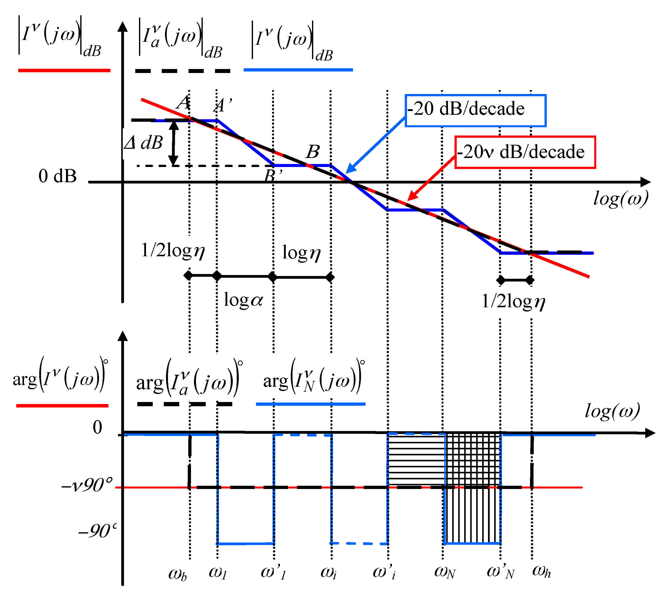
As shown by Figure 1, the Bode plots of relation (2) exhibit:
- -
- a gain whose slope is a fractional multiple of −20 dB/decade,
- -
- a constant phase whose value is a fractional multiple of −90°.
These Bode plots can be approximated using a distribution of poles and zeros. This leads to the following algorithm (Algorithm 1).
| Algorithm 1. Fractional integrator approximation—first method | |
| 1. Initialize 3. Compute | |
As shown in [26], with this algorithm, the corner frequencies and (respectively the poles and zeros of the transfer function ) are geometrically distributed to obtain the required frequency behavior.
Figure 1 highlights this distribution and also compares the asymptotic Bode plots of , and . It also shows that the high and low asymptotic frequency behaviors are constant. In [22], to obtain an integer integral like asymptotic behavior at low and high frequency, relation (2) is replaced by:
This leads to the following algorithm (Algorithm 2).
| Algorithm 2. Fractional integrator approximation—second method | |
| 1. Initialize 3. Compute with relation (5) 4. Define the fractional integrator (1) approximation in the frequency band [ωb, ωh], by the transfer function | |
For a fractional differentiation operator defined in the Laplace domain by
the frequency truncation leads to
and permits the following algorithm (Algorithm 3).
| Algorithm 3. Fractional differentiator approximation—first method | |
| 1. Initialize 3. Compute with relation (5) 4. Define the fractional differentiator (12) approximation in the frequency band [ωb, ωh], by the transfer function | |
By analogy with Algorithm 2, the following algorithm (Algorithm 4) permits to get an integer differentiation like asymptotic behavior in low and high frequency.
| Algorithm 4. Fractional differentiator approximation—second method | |
| 1. Initialize 3. Compute with relation (5) 4. Define the fractional differentiator (12) approximation in the frequency band [ωb, ωh], by the transfer function | |
The set of algorithms previously established for a real fractional differentiation order can be extended to a complex fractional differentiation order ν = a + ib [21].
2.2. Approximation of a Fractional Integrator by a Recursive Distribution of Poles and Zeros: An Analytical Approach
For the approximation given in relation (1) using Algorithm 1, the analytical demonstration of the graphical approach presented in the previous section was done in [21] by considering the limit case where ωb tends towards 0 and ωh tends towards infinity. However, a simpler demonstration based on the impulse response of a fractional operator is now used. This impulse response is defined by:
where denotes the inverse Laplace–Transform. The residue method for the computation of the inverse Laplace–Transform leads to [3]:
The Laplace–Transform of (19) is thus given by:
Using the change of variable and thus , then:
Discretization of integral (22) leads to:
in which denotes the sampling interval. Relation (22) also highlights the link between a fractional integrator impulse response and the Prony series as the inverse Laplace transform of (23) leads to:
with and .
Relation (24) also highlights that the poles αk (always greater than 0) are linked by the ratio αk+1/αk = e−Δz. Regarding the zeros, to the best of the author’s knowledge there is no demonstration of a link with the same ratio as that imposed by Algorithm 1. However, by applying a partial fraction decomposition to relation (3) it can be written as:
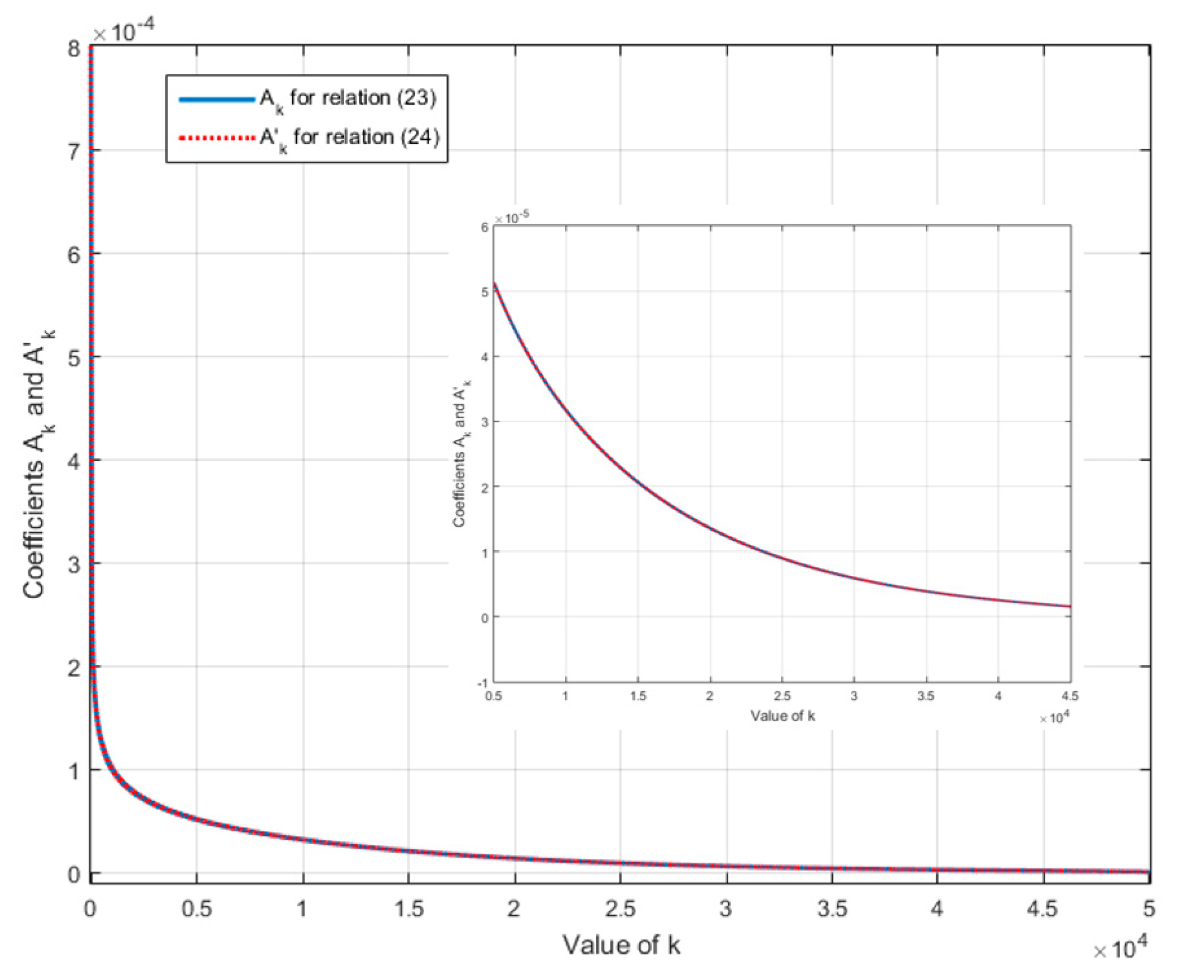
By choosing α′k = αk, it can be shown using a graphical representation (see Figure 2) that coefficient A′k in relation (25) tends towards coefficient Ak in (24), under the same hypothesis as the one used in [21]:
- -
- a number N of poles that tends towards infinity,
- -
- a ratio r or Δz that tends towards 1.
3. Sub-Optimality of Algorithms 1–4 and Beyond Geometric Distribution
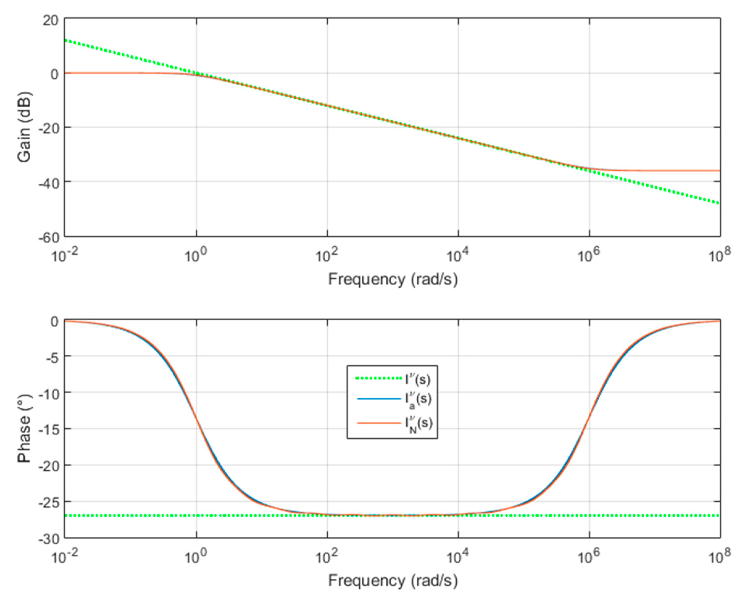
The algorithms 1 to 4 described in Section 2 have been used in many applications, due to the simplicity of their implementation. However, it can be demonstrated by an example that Algorithm 1, for instance, is sub-optimal (a similar demonstration can be made for Algorithms 2 to 4). Let us assume that the aim is to compute the approximation of transfer function (1) on the frequency band [ωb, ωh] = [1, 106], with ν = 0.3. Using Algorithm 1 with N = 10 poles and zeros, the following factors are obtained:
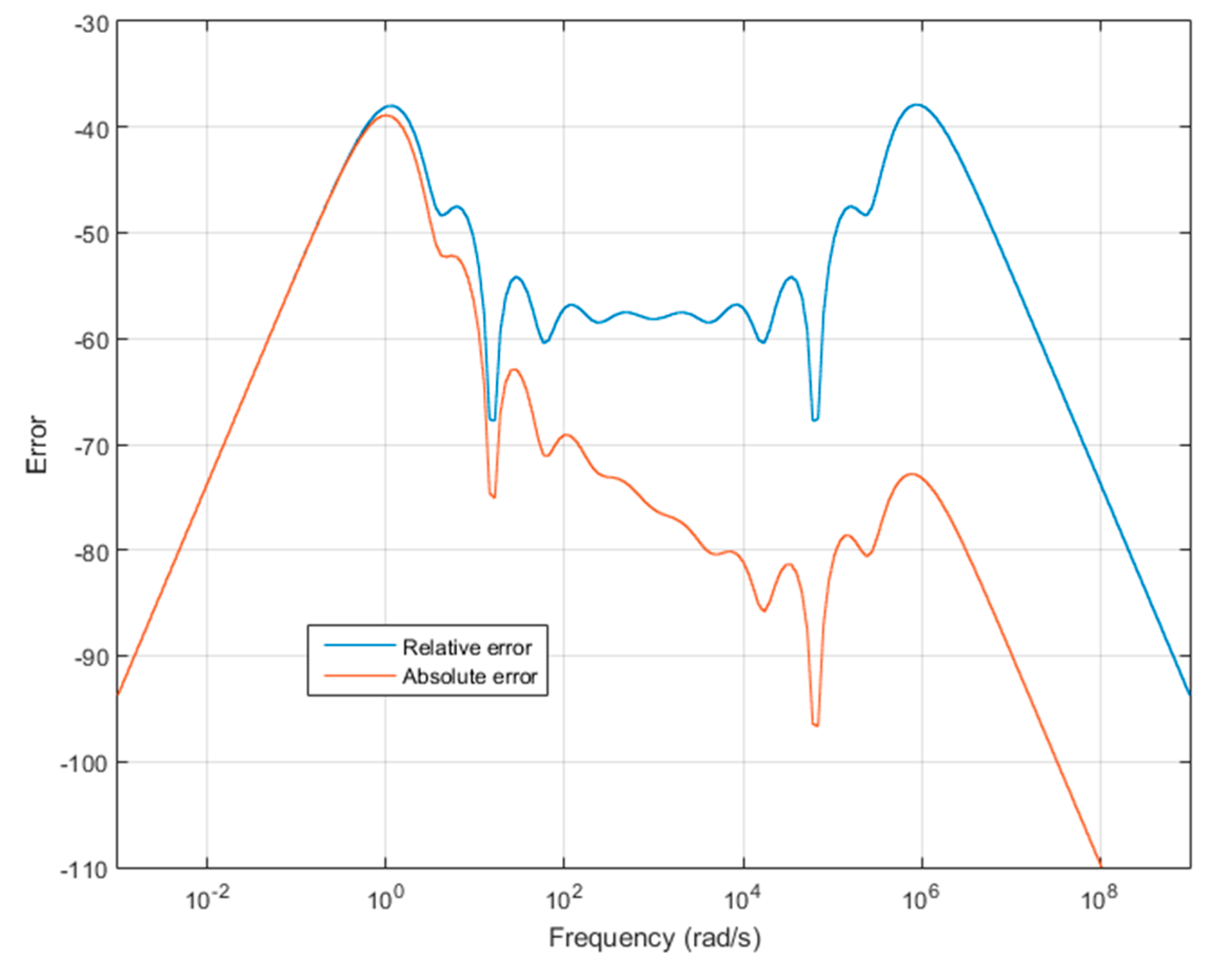
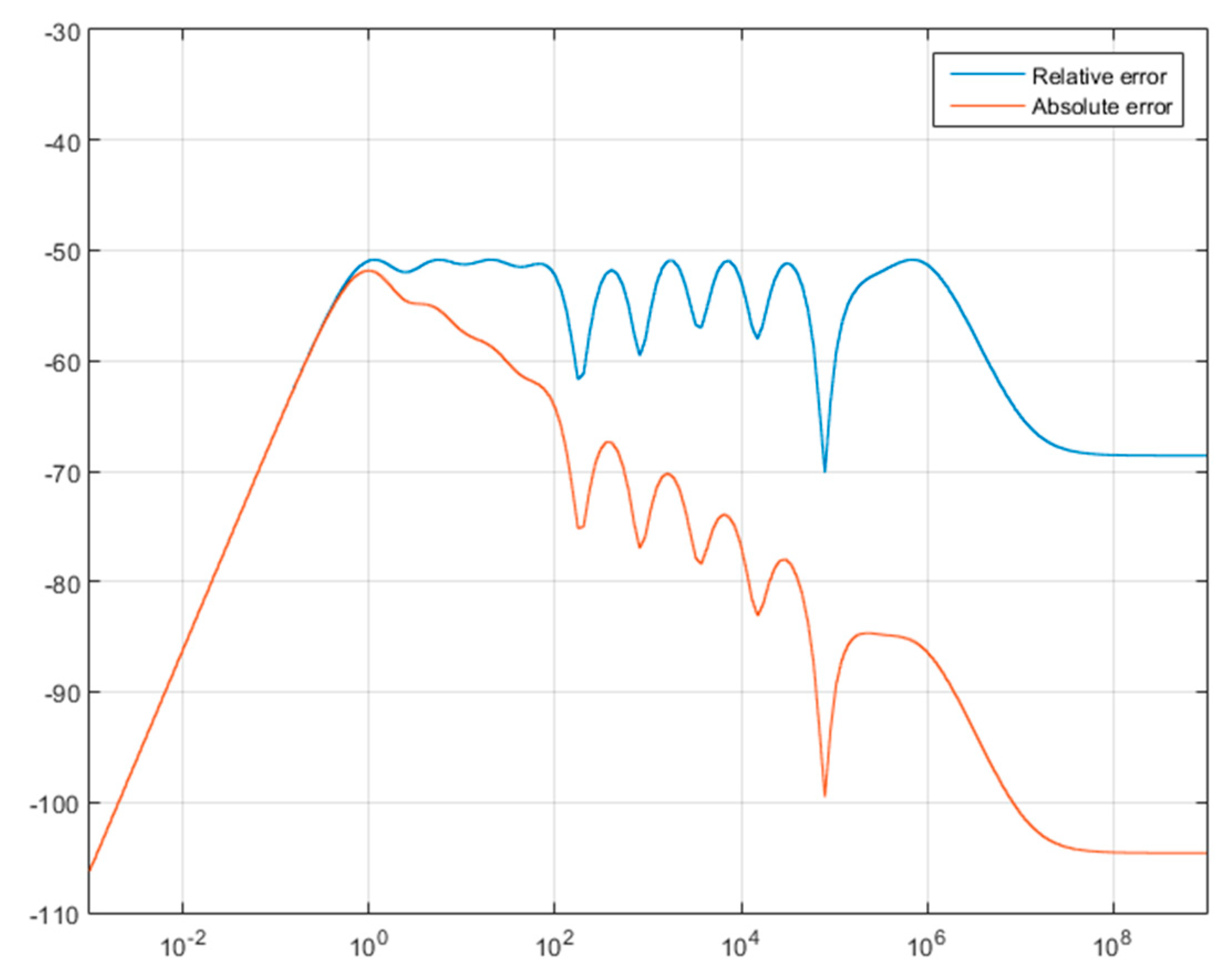
which enable all the corner frequencies of relation (3) to be computed using relations (4) and (5). The Bode plots of relations (1) to (3) are represented by Figure 3. To evaluate the efficiency of Algorithm 1, the relative error and absolute error respectively computed by the relations
are represented by Figure 4. The maximum values of and are respectively given by:
Then, an optimization program aiming at reducing the relative error by looking for the best location of the N poles and zeros in the transfer function is implemented under a Matlab environment. The optimization program is initialized with the pole and zero values obtained with Algorithm 1. The resulting relative error and absolute error are shown in Figure 5. The maximum values of and are now respectively given by:
and are almost five times smaller than the ones given by Algorithm 1.
To improve the accuracy of Algorithms 1–4, it is necessary to go beyond the geometric distribution of poles and zeros, but without introducing great complexity. With N poles , to define these generalizations, let us define the ratio r such that:
For a geometric distribution, the following relation holds:
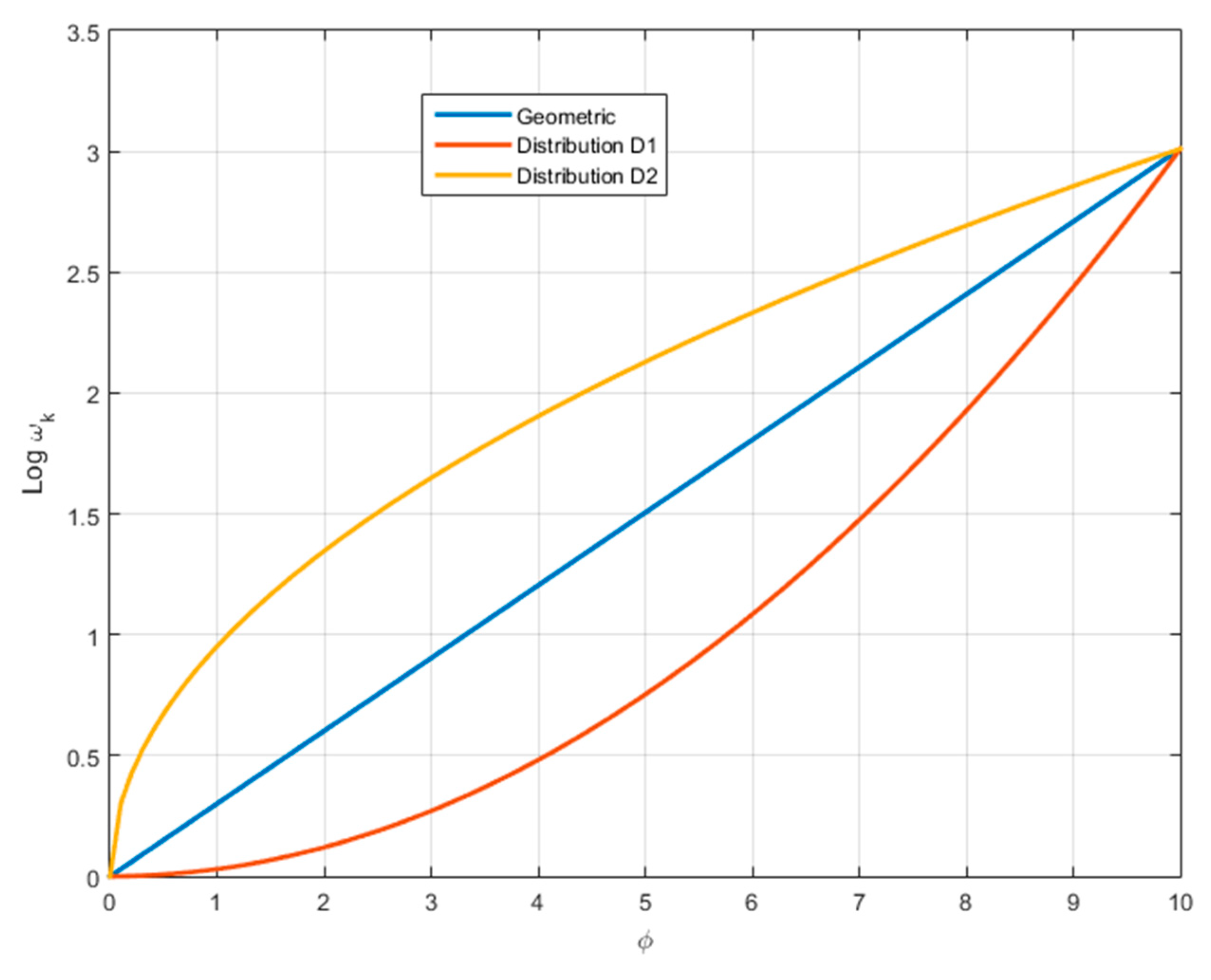
It can be generalized, among many others, by the following distributions:
In Figure 6, these two distributions are compared with the geometric one. It shows that distribution D1 makes it possible to bring the first poles closer together while distribution D2 makes it possible to increase the distance between them. However, no additional tuning parameters are associated to these distributions. It is thus proposed to replace the nonlinear function of N in relations (32) and (33) by a polynomial. The following distribution is thus obtained:
With M = 2, to ensure that corner frequencies really belong in , the following constraints must be imposed: P(0) = 0 and P(N) = N. This leads to imposing a0 = 0 and a1N + a2N2 = N, thus a2 = (1 − a1)/N.
With M = 3, to ensure that corner frequencies really belong in , the same constraints must be imposed leading to a0 = 0 and . Moreover, if it is imposed that distribution D3 fits the geometric distribution in the middle of the interval , the following constraint must be added: P(N/2) = 1/2 and thus . Finally, parameters a2 and a3, meet the following system of equations:
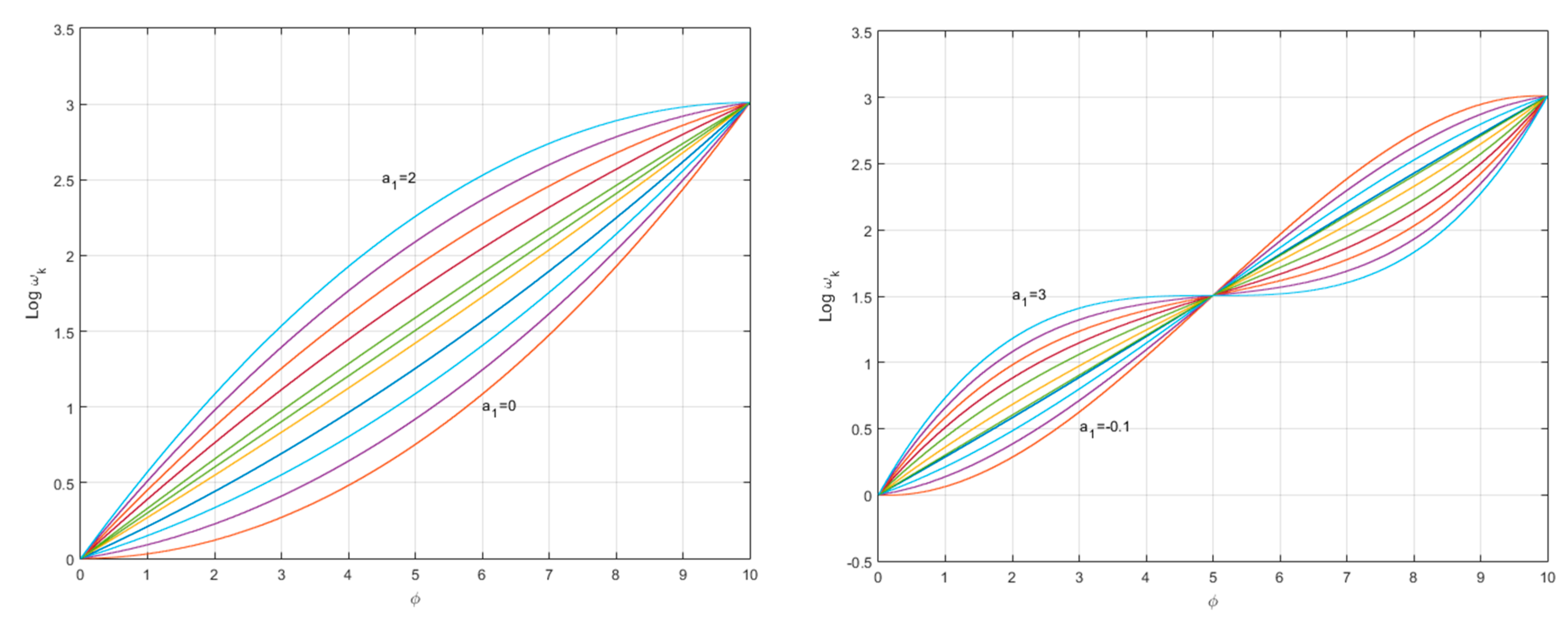
By varying parameter a1, Figure 7 shows the large number of distributions that can be obtained in both cases.
In the two cases, it must be pointed out that only one parameter needs to be tuned to obtain a wide variety of distributions.
For the geometric distribution, according to Algorithm 1, the poles, and zeros in relation (3) are defined by relation (34) with
and
To define the poles and the zeros using the distribution introduced, the same values of φ are used, but the values of and are given by relation (34) leading to the following algorithm (Algorithm 5).
| Algorithm 5. Fractional integrator approximation—improved method | |
| 1. Initialize 3. Compute with relation (5) 4. Define the fractional integrator (1) approximation in the frequency band [ωb, ωh], by the transfer function | |
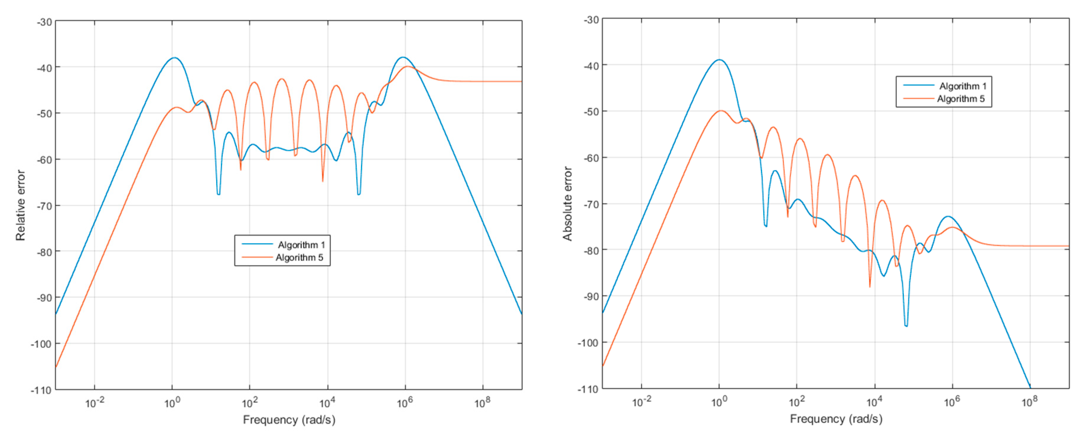
The efficiency of this algorithm is highlighted on the example used at the beginning of Section 3, but with a distribution D3 and M = 3. The parameter a1 is computed to reduce the relative error given in relation (27). Given that only one parameter has to be found, it is done by a gridding of parameter a1 on the interval [−0.1, 3]. A comparison of relative and absolute errors obtained with Algorithms 1 and 5 is given in Figure 8. The maximum values of these absolute and relative errors are given by:
In comparison with Algorithm 1, these values are greatly reduced with Algorithm 5.
4. Fractional Model Approximation and Stability Issues
We now consider a fractional order model described by the pseudo state space description,
where is the pseudo state vector, is the fractional order of the system and , , and are constant matrices. A solution for the implementation of such a model consists in the approximation of the fractional order derivative by the approximation given by Algorithm 3 or Algorithm 4. However, such an approximation has an impact on model stability. It is well known that model (43) is stable if and only if all the eigenvalues of matrix A belong to the stability domain Ds defined by:
To explain how the stability domain is transformed by approximation (15) in Algorithm 3 or (18) in Algorithm 4, it is assumed that all the eigenvalues of model (43) are distinct. Thus, there exists a change of variable z(t) = P x(t), such that model (43) can be written as:
where matrix Ap is diagonal and can be written , . Using the Laplace transform, the characteristic equations of model (45) are thus
with approximation (15) or (18), these characteristic equations become:
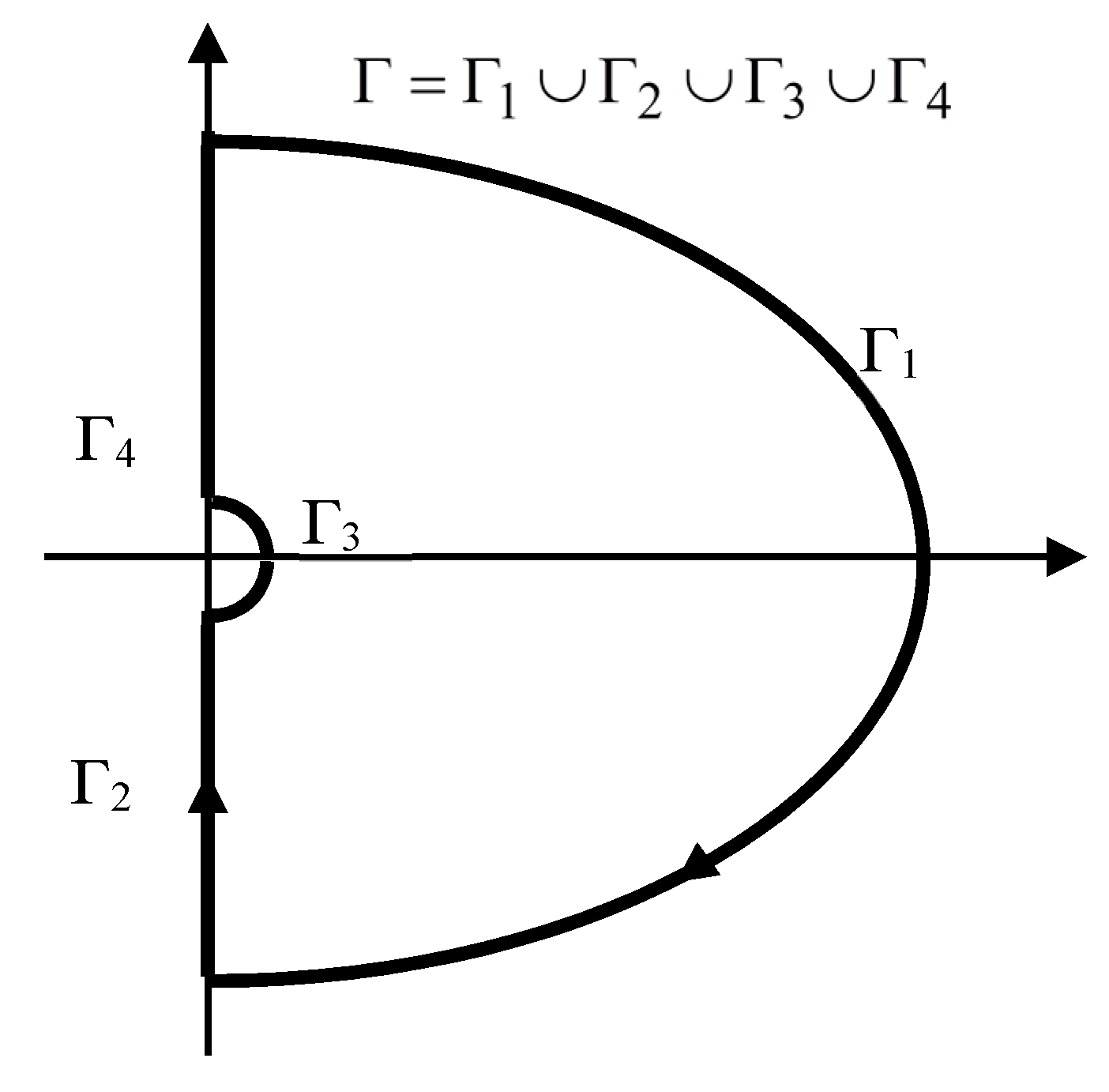
After approximation, model (43) is stable if characteristic Equation (47) has no root in the right half part of the complex plane. To evaluate the location of these roots, the Cauchy argument principle can be used. For that, the path Г in Figure 9 can be used.
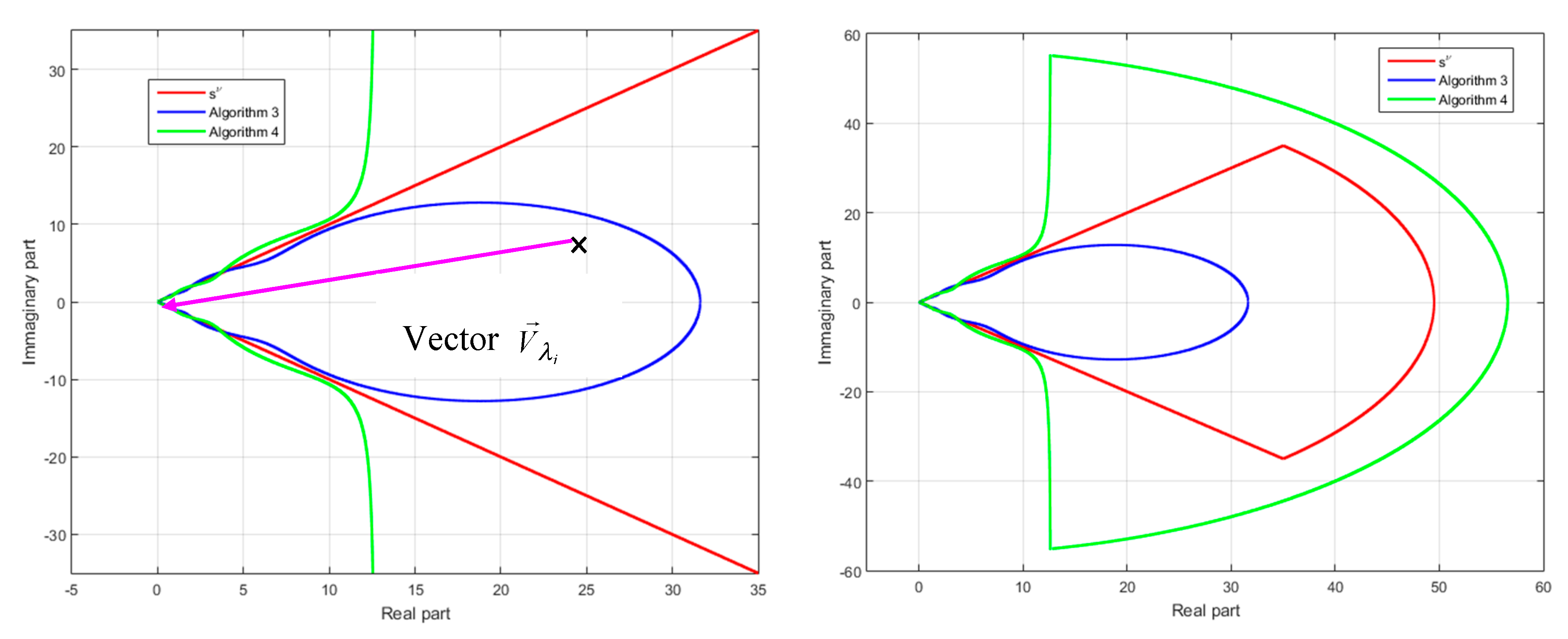
Images of path Г by approximations (15) and (18) are represented by Figure 10. They are compared with the image of this path by sν.
From these curves, the stability domain of model (43) can be deduced. The image of path Г by relation (47) is the image of path Г by relations (15) and (18) translated by the vector that appears in Figure 10 and that links the point of the coordinate (Re(λi), Im(λi)) to the origin of the complex plane. Thus, after this translation the origin of the complex plane is located at the point (Re(λi), Im(λi)). As the denominator of relations (47) has no root inside the path Г, if the origin (after translation) of the complex plane is inside one of the images, then according to argument principle, the corresponding characteristic equation has one root inside the path Г and the system (43) is unstable. This permits the following theorem.
Theorem 1.
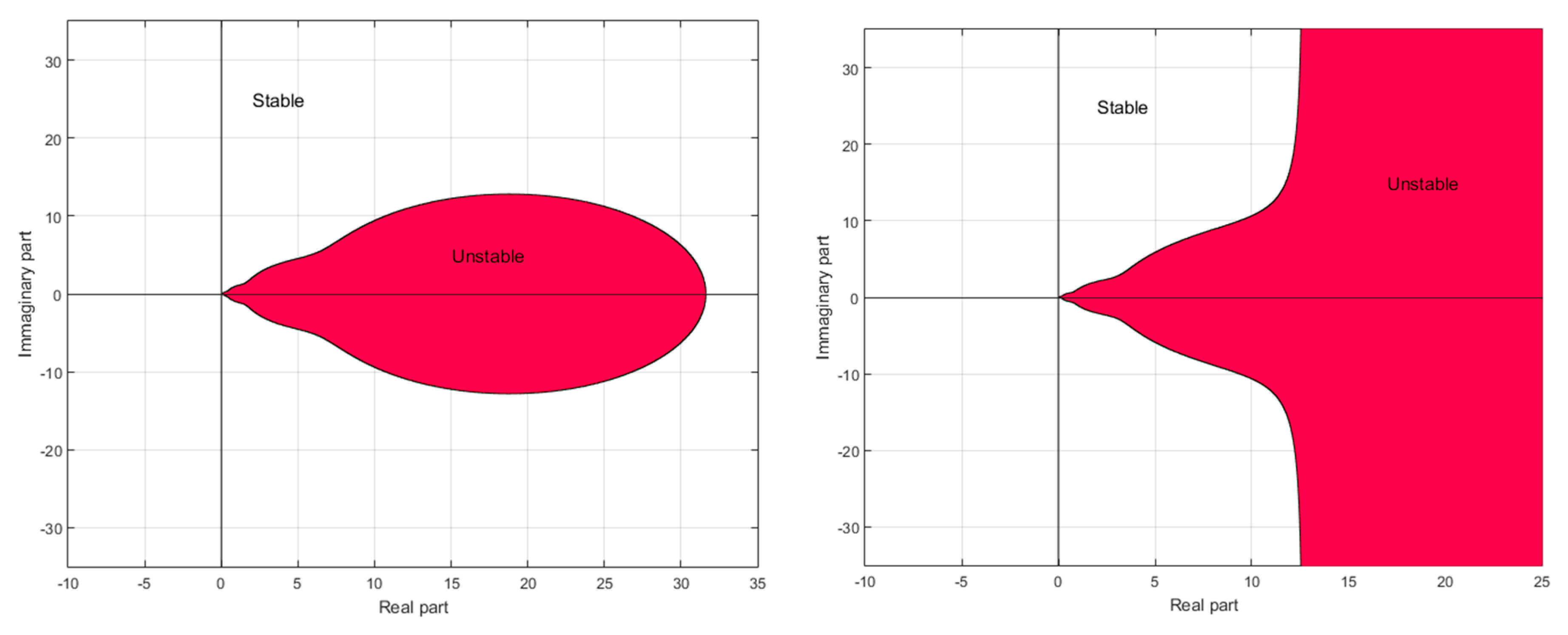
The stability domain in the complex plane, for the eigenvalues of matrix AP (or for the poles) of model (45) or equivalently for model (43) is
- -
- outside the domain defined by,,,for approximation (15)
- -
- outside the domain on the right of the curve,,, for approximation (18).
These stability domains are illustrated by Figure 11.
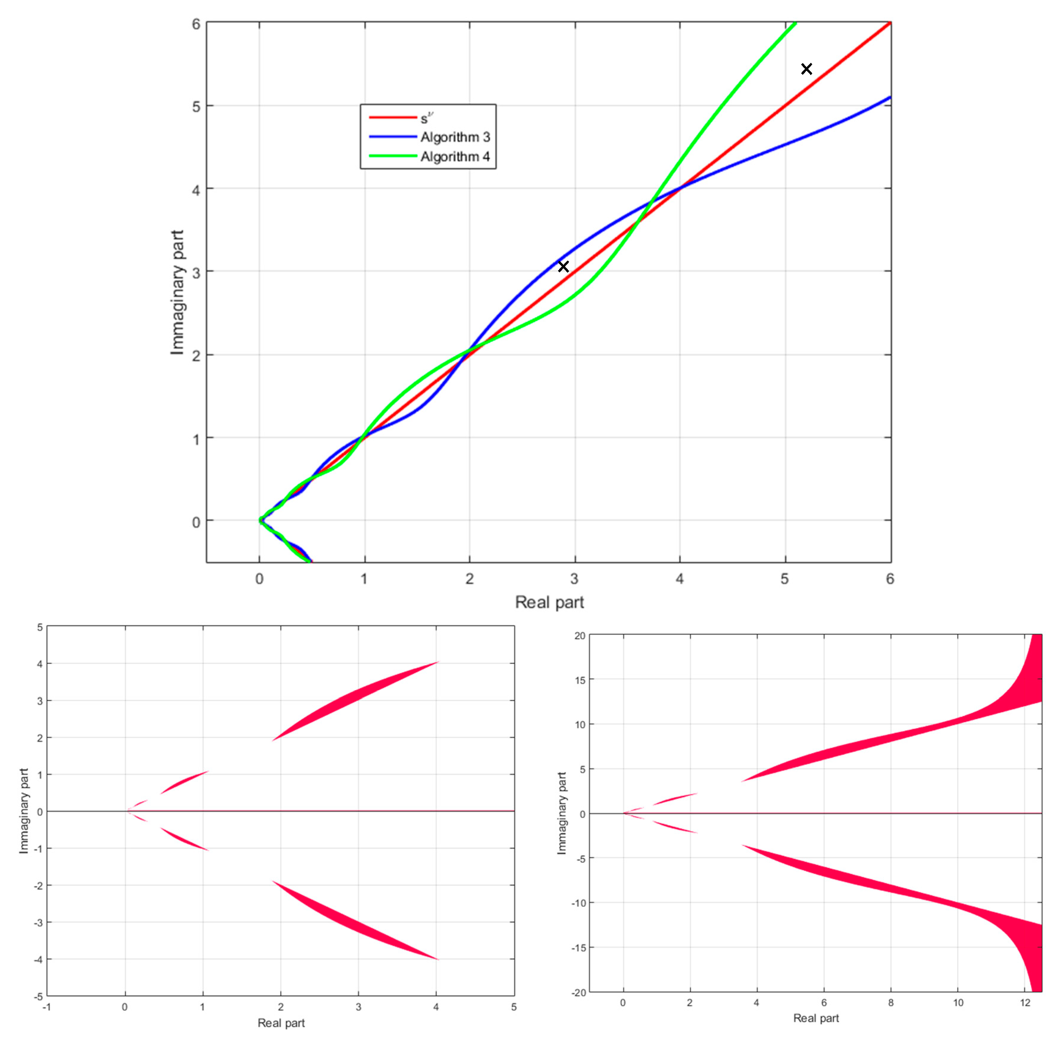
This analysis also highlights stability issues that can occur after approximation. Considering Figure 12, which is an enlargement of Figure 11, it can be seen that some instability domains for model (43) after approximation are inside the stability domains for model (43) (before approximation). Some of these areas are marked with crosses on this figure. As a conclusion, approximation of a stable model using approximations (15) or (18) can produce an unstable model if some eigenvalues are located outside the intersections of the various stability domains.
To avoid such a situation, a careful analysis of the fractional model eigenvalues is required before approximation.
5. Conclusions
Geometric (or recursive) pole and zero distribution is a solution often found in the literature for the approximation of fractional order models. Some writers even go so far as to say that “recursivity (in the sense of geometric distribution) is fundamental in the non-integer differentiation synthesis” ([29], p. 165). Such an assertion is questionable. It is indeed shown in this paper that this distribution and the associated algorithms for its computation:
- -
- result in the discretization of the impulse response of a fractional model,
- -
- are sub-optimal,
- -
- are one among an infinity of other permitted distributions.
The paper thus proposes several other distributions for the approximation of fractional operators and fractional models. It also shows that the geometric distribution found in the literature leads to stability issues after approximation that can be avoided by an analysis of the pole location (in the complex plane) of the fractional model before approximation.
For all these reasons, it cannot be said that this “recursivity” is the physical reason for the observed long memory behaviors as is sometime claimed for the modeling of capacitors [29] or other systems, and the author is currently exploring stochastic reasons.
Funding
This research received no external funding.
Conflicts of Interest
The author declares no conflict of interest.
References
- Oldham, K.B.; Spanier, J. The Fractional Calculus; Theory and Applications of Differentiation and Integration to Arbitrary Order (Mathematics in Science and Engineering, V); Academic Press: Cambridge, MA, USA, 1974. [Google Scholar]
- Samko, S.G.; Kilbas, A.A.; Marichev, O.I. Fractional Integrals and Derivatives: Theory and Applications; Gordon and Breach Science Publishers: Philadelphia, PA, USA, 1993. [Google Scholar]
- Podlubny, I. Fractional differential equations. In Mathematics in Sciences and Engineering; Academic Press: Cambridge, MA, USA, 1999. [Google Scholar]
- Rodrigues, S.; Munichandraiah, N.; Shukla, A.K. A review of state-of-charge indication of batteries by means of a.c. impedance measurements. J. Power Sources 2000, 87, 12–20. [Google Scholar] [CrossRef]
- Jocelyn Sabatier, J.; Mohamed, A.; Oustaloup, A.; Grégoire, G.; Ragot, F.; Roy, P. Fractional system identification for lead acid battery state charge estimation. Signal Process. 2006, 86, 2645–2657. [Google Scholar] [CrossRef]
- Sabatier, J.; Merveillaut, M.; Francisco, J.; Guillemard, F. Lithium-ion batteries modelling involving fractional differentiation, Journal of power sources. J. Power Sources 2014, 262, 36–43. [Google Scholar] [CrossRef]
- Dlugosz, M.; Skruch, P. The application of fractional-order models for thermal process modelling inside buildings. J. Build. Phys. 2016, 39, 440–451. [Google Scholar] [CrossRef]
- Sabatier, J.; Farges, C.; Fadiga, L. Approximation of a fractional order model by an integer order model: A new approach taking into account approximation error as an uncertainty. J. Vib. Control 2016, 22, 2069–2082. [Google Scholar] [CrossRef]
- Magin, R. Fractional Calculus in Bioengineering; Begell House Publishers: Danbury, CT, USA, 2006. [Google Scholar]
- Mainardi, F. Fractional Calculus and Waves in Linear Viscoelasticity; Imperial College Press: London, UK, 2010. [Google Scholar]
- Matignon, D.; D’Andréa-Novel, B.; Depalle, P.; Oustaloup, A. Viscothermal losses in wind instruments: A non-integer model. Math. Res. 1994, 79, 789. [Google Scholar]
- Fonseca Ferreira, N.M.; Duarte, F.B.; Miguel, F.M.; Lima, M.F.M.; Marcos, M.G.; Tenreiro Machado, J.A. Application of fractional calculus in the dynamical analysis and control of mechanical manipulators. Fract. Calc. Appl. Anal. J. 2008, 11, 91–113. [Google Scholar]
- Enacheanu, O.; Riu, D.; Retiere, N. Half-order modelling of electrical networks Application to stability studies. IFAC Proc. Vol. 2008, 41, 14277–14282. [Google Scholar] [CrossRef]
- Gruau, C.; Picart, D.; Belmas, R.; Bouton, E.; Delmaire-Size, F.; Sabatier, J.; Trumel, H. Ignition of a confined high explosive under low velocity impact. Int. J. Impact Eng. 2009, 36, 537–550. [Google Scholar] [CrossRef] [Green Version]
- Sabatier, J.; Merveillaut, M.; Malti, R.; Oustaloup, A. On a Representation of Fractional Order Systems: Interests for the Initial Condition Problem. In Proceedings of the 3rd IFAC Workshop on “Fractional Differentiation and its Applications” (FDA’08), Ankara, Turkey, 5–7 November 2008. [Google Scholar]
- Sabatier, J.; Merveillaut, M.; Malti, R.; Oustaloup, A. How to Impose Physically Coherent Initial Conditions to a Fractional System? Commun. Nonlinear Sci. Numer. Simul. 2010, 15, 1318–1326. [Google Scholar] [CrossRef]
- Sabatier, J.; Farges, C.; Trigeassou, J.C. Fractional systems state space description: Some wrong ideas and proposed solutions. J. Vib. Control 2014, 20, 1076–1084. [Google Scholar] [CrossRef]
- Sabatier, J.; Farges, C. Comments on the description and initialization of fractional partial differential equations using Riemann-Liouville’s and Caputo’s definitions. J. Comput. Appl. Math. 2018, 339, 30–39. [Google Scholar] [CrossRef]
- Sabatier, J.; Farges, C.; Merveillaut, M.; Feneteau, L. On observability and pseudo state estimation of fractional order systems. Eur. J. Control 2012, 18, 1–12. [Google Scholar] [CrossRef]
- Malti, R.; Sabatier, J.; Akçay, H. Thermal modeling and identification of an aluminum rod using fractional calculus. In Proceedings of the 15th IFAC Symposium on System Identification, Saint-Malo, France, 6–8 July 2009; pp. 958–963. [Google Scholar]
- Oustaloup, A.; Levron, F.; Mathieu, B.; Nanot, F. Frequency-band complex non integer differentiator: Characterization and synthesis. IEEE Trans. Circuits Syst. I Fundam. Theory Appl. 2000, 47, 25–39. [Google Scholar] [CrossRef]
- Poinot, T.; Trigeassou, J.-C. A method for modelling and simulation of fractional systems. Signal Process. 2003, 83, 2319–2333. [Google Scholar] [CrossRef]
- Manabe, S. The non-integer Integral and its Application to control systems. ETJ Jpn. 1961, 6, 83–87. [Google Scholar]
- Carlson, G.E.; Halijak, C.A. Simulation of the Fractional Derivative Operator and the Fractional Integral Operator. Available online: http://krex.k-state.edu/dspace/handle/2097/16007 (accessed on 30 June 2018).
- Ichise, M.; Nagayanagi, Y.; Kojima, T. An analog simulation of non-integer order transfer functions for analysis of electrode processes. J. Electroanal. Chem. Interfacial Electrochem. 1971, 33, 253–265. [Google Scholar] [CrossRef]
- Oustaloup, A. Systèmes Asservis Linéaires d’ordre Fractionnaire; Masson: Paris, France, 1983. [Google Scholar]
- Raynaud, H.F.; Zergaïnoh, A. State-space representation for fractional order controllers. Automatica 2000, 36, 1017–1021. [Google Scholar] [CrossRef]
- Charef, A. Analogue realisation of fractional-order integrator, differentiator and fractional PI/^ lambda/D/^ mu/ controller. IEE Proc. Control Theory Appl. 2006, 153, 714–720. [Google Scholar] [CrossRef]
- Oustaloup, A. Diversity and Non-integer Differentiation for System Dynamics; Wiley: Hoboken, NJ, USA, 2014. [Google Scholar]
Figure 1.
Bode plots comparison of , and .

Figure 2.
Comparison of coefficients A′k in relation (25) which tends towards coefficients Ak in (24) and zoom inside the figure.
Figure 2.
Comparison of coefficients A′k in relation (25) which tends towards coefficients Ak in (24) and zoom inside the figure.

Figure 3.
Bode plot comparison of , and .

Figure 4.
Gain plot of relative error and absolute error.

Figure 5.
Gain plots of relative error and absolute error after optimization.

Figure 6.
Two examples of pole distributions compared to the geometric one.

Figure 7.
Two examples of pole distributions with D3: M = 2 (left), M = 3 (right).

Figure 8.
Comparison of relative (left) and absolute (right) errors between Algorithms 1 and 5 with distribution D3.
Figure 8.
Comparison of relative (left) and absolute (right) errors between Algorithms 1 and 5 with distribution D3.

Figure 9.
Considered path Г.

Figure 10.
Image of path Г by approximations (15) and (18): definition of vector on a zoom (left), full contour image (right).
Figure 10.
Image of path Г by approximations (15) and (18): definition of vector on a zoom (left), full contour image (right).

Figure 11.
Stability domains for the eigenvalues of model (43) with approximation (13) (left) and approximation (18) (right).
Figure 11.
Stability domains for the eigenvalues of model (43) with approximation (13) (left) and approximation (18) (right).

Figure 12.
Impact of approximations (15) and (18) on stability model (43): illustration of stability issues (top), and problematic areas of the complex plane for approximation (15) (bottom left) and for approximation (18) (bottom right).
Figure 12.
Impact of approximations (15) and (18) on stability model (43): illustration of stability issues (top), and problematic areas of the complex plane for approximation (15) (bottom left) and for approximation (18) (bottom right).

© 2018 by the author. Licensee MDPI, Basel, Switzerland. This article is an open access article distributed under the terms and conditions of the Creative Commons Attribution (CC BY) license (http://creativecommons.org/licenses/by/4.0/).
Share and Cite
MDPI and ACS Style
Sabatier, J. Solutions to the Sub-Optimality and Stability Issues of Recursive Pole and Zero Distribution Algorithms for the Approximation of Fractional Order Models. Algorithms 2018, 11, 103. https://doi.org/10.3390/a11070103
AMA Style
Sabatier J. Solutions to the Sub-Optimality and Stability Issues of Recursive Pole and Zero Distribution Algorithms for the Approximation of Fractional Order Models. Algorithms. 2018; 11(7):103. https://doi.org/10.3390/a11070103
Chicago/Turabian StyleSabatier, Jocelyn. 2018. "Solutions to the Sub-Optimality and Stability Issues of Recursive Pole and Zero Distribution Algorithms for the Approximation of Fractional Order Models" Algorithms 11, no. 7: 103. https://doi.org/10.3390/a11070103
Note that from the first issue of 2016, this journal uses article numbers instead of page numbers. See further details here.