An Ensemble Extreme Learning Machine for Data Stream Classification

Abstract

Extreme learning machine (ELM) is a single hidden layer feedforward neural network (SLFN). Because ELM has a fast speed for classification, it is widely applied in data stream classification tasks. In this paper, a new ensemble extreme learning machine is presented. Different from traditional ELM methods, a concept drift detection method is embedded; it uses online sequence learning strategy to handle gradual concept drift and uses updating classifier to deal with abrupt concept drift, so both gradual concept drift and abrupt concept drift can be detected in this paper. The experimental results showed the new ELM algorithm not only can improve the accuracy of classification result, but also can adapt to new concept in a short time.

1. Introduction

With the explosively growing Internet and rapid development of information society, many industries have generated a large number of data streams, such as medical diagnosis, online shopping, traffic flow detection and satellite remote sensing. Different from conventional static data, data streams often have the characteristics of infinite quantity, rapid arrival, and conceptual drift, which make data stream mining faces an enormous challenges [1,2,3]. Since data stream classification was put forward, it has attracted much attention from scholars and made many achievements [4,5,6,7,8,9]. Up to now, the achievements are divided into three groups: statistical analysis model, decision tree model and neural network model. In statistical analysis model, Brzezinski et al. proposed an online leaning algorithm called OAUE [10] which utilizes mean square error to determine the weight of the classification model. When the detection period is reached, the concept drift will be replaced by replacement strategy. Farid et al. proposed a weighted case ensemble classification algorithm [11], and clustering algorithm is introduced to detect concept drift. If a data point does not belong to any existing class, it is considered that the class corresponding to this data may be a new concept, and then is further confirmed by data statistics in nodes. Bifet et al. proposed an adaptive window algorithm called HWF-ADWIN [12]. It uses Hoeffding inequality [13] to divide the nodes with the attributes corresponding to the maximum and second largest information gain to train a classifier; when the accuracy of the classifier is significantly changed, concept drift will be thought to have happened. Xu et al. proposed a data stream classification method based on Kappa coefficient [14]; in the process of classification, the algorithm calculates the Kappa coefficients of each block, and detects the changes of concepts in data streams by using Kappa coefficients. When the concept of data stream is changing, the system will eliminate the classifiers which do not meet the requirements according to the existing knowledge. Compared with the contrast algorithm, this algorithm can not only obtain a higher accuracy, but also reduce the time cost to a certain extent, and get better results. Decision tree model is very common in data stream classification tasks and there have been many publications. Domingos and Hulten et al. proposed a series of algorithms based on Hoeffding tree called VFDT and CVFDT [15,16]; Wu and Li et al. proposed semi-random decision tree algorithms [17,18]; Brzezinski et al. proposed a red–black tree structure algorithm to improve the efficiency of finding and removing outdated nodes for imbalanced data stream classification [19]. Rutkowski et al. developed a McDiarmid Tree algorithm according to McDiarmid inequality and the threshold of the difference between the maximum information gain and the second large information gain is determined by the McDiarmid boundary [20]. With the heat of the neural network, many scholars apply neural network in data stream classification tasks. Aiming at imbalanced data stream classification [21], telecommunication fraud detection [22], spatiotemporal event streams [23] and so on, many algorithms have been proposed. However, statistical analysis model, decision tree model and neural network model need to repeatedly scan data classifiers and data several times, or there are many parameter needing to adjustment. Thus, the above drawbacks limit these models to be more widely used in data stream environment.

Extreme learning machine is a single hidden layer feedforward neural network; the input weights and biases of hidden layer are randomly generated and the output weights can be automatically determined by input data [24,25,26,27,28]. ELM does not need to adjust the parameters repeatedly and it has an obvious advantage in the speed of the training process comparing with the traditional neural networks [29], so it is very suitable for data stream classification tasks. Liang et al. proposed an ELM algorithm based on online sequential learning mechanism called OS-ELM [30], and it extends ELM to the field of data stream classification. After OS-ELM being proposed, many scholars have proposed a series of improved OS-ELM. Gu et al. proposed a timeliness online sequential extreme learning machine for timeliness problem [31]; it adopts the batch processing and weighting mechanism to make TOSELM have good stability and prediction ability. Shao et al. proposed a regularization extreme learning machine with online sequential learning called OS-RELM [32]. OS-RELM combines OS-ELM and RELM [33]; at the same time, the minimum error rate is guaranteed, and the norm of the minimum weight is obtained, so that OS-RELM can have good generalization performance. Zhao et al. proposed a FOS-ELM with forgetting mechanism for timeliness stock data [34]. In FOS-ELM, it only uses latest data to update model, so it can avoid the invalid data to participate in updating the weights of the output layer. Bilal et al. proposed an ensemble online sequential extreme learning machine for imbalanced classification [35]; each OS-ELM focuses on the minority class data and is trained with a balanced subset of the data stream. For distributed multi-agent system, Vanli et al. proposed a online nonlinear extreme learning machine [36]; it uses optimization method to minimize empirical risk and structural risk. Singh et al. applied OS-ELM in intrusion detection system [37]; before dealing with data, it introduces features selection to eliminate redundant or unrelated attributes.

The above OS-ELM and its developments provide a number of ways to solve the problem of data stream classification. However, most of them lack concept drift detection mechanism; they have a good performance for data stream without concept drift or concept changing slowly, but cannot cope with the rapid change of concept in data stream. In this paper, an ensemble extreme learning machine with concept drift detection (CELM) is proposed. CELM uses manifold learning to reduce the dimensions of data and introduces concept drift detection mechanism which effectively overcomes the shortcomings of OS-ELM. The contributions of this paper are as follows:

• An ensemble extreme learning machine algorithm is presented. In the data stream environment, the performance of ensemble classifiers is better than that of single classifier [38], so CELM employs ensemble learning method and improves the performance of ELMs.
• Because data stream classification is very demanding for real time and the high dimensions of data tend to reduce the efficiency of algorithm, CELM introduces a manifold learning method to reducing the dimension of data which reduces the time consumption of CELM.
• Concept drift detection is incorporated into the training process of ELM classifiers. The change of data stream is divided into three categories: normal condition, warning level and concept drift. Different from the traditional ELMs, CELM not only can detect gradual concept drift, but also can handle abrupt concept drift.

The rest of this paper is organized as follows: Section 2 reviews the background knowledge of data stream classification and ELM. Section 3 states the details of ELM, and then elaborates the reducing dimension method of the manifold learning and the principles of CELM. In Section 4, CELM is compared with comparison algorithms and we discusses the experimental results. Finally, Section 5 concludes the research and gives future directions.

2. Background Knowledge

In this section, we give a brief introduction about data stream classification and extreme learning machine and explain their basic principles.

2.1. Data Stream Classification

Let $\left\{\cdots ,{\mathit{d}}_{t-1},{\mathit{d}}_t,{\mathit{d}}_{t+1},\cdots \right\}$ be a data stream generated by a system, and ${\mathit{d}}_t$ a datum at t moment; ${\mathit{d}}_t=\left\{x_{t1},x_{t2},\cdots ,x_{tm},y_t\right\}$, where m is the features number of ${\mathit{d}}_t$ and $y_t$ is the class label. Data stream classification generally adopts a sliding window mechanism, and several data make up a dataset called data block and denoted ${\mathit{B}}_i$, where ${\mathit{B}}_i=\left\{d_{\left(1\right)},d_{\left(2\right)},\cdots ,d_{\left(n\right)}\right\}$ and n is the size of data block. At every moment, only one or several data blocks are allowed to enter sliding window. After one data block is processed, a new data block can be loaded to sliding window.

Suppose that in $\Delta t$ time, if the error rate of classifier system is at a low level in the sliding window, it is said that the concept of data stream is stable in this period and $P\left(error-best\le \epsilon \right)\ge 1-\alpha$, where error is the current error rate of classifier system, best is the classification error rate of optimal performance classifier for data stream and $\alpha$ is a significance level. Let the classification model of data stream be M, which is trained by the data blocks in sliding window at t moment; after $\Delta t$ time, the classification model changes to N. If $M\ne N$, it means concept drift has happened in data stream. If $\Delta t$ is a short time, the concept drift is called abrupt concept drift; otherwise, it is called as gradual concept drift [14].

2.2. Extreme Learning Machine

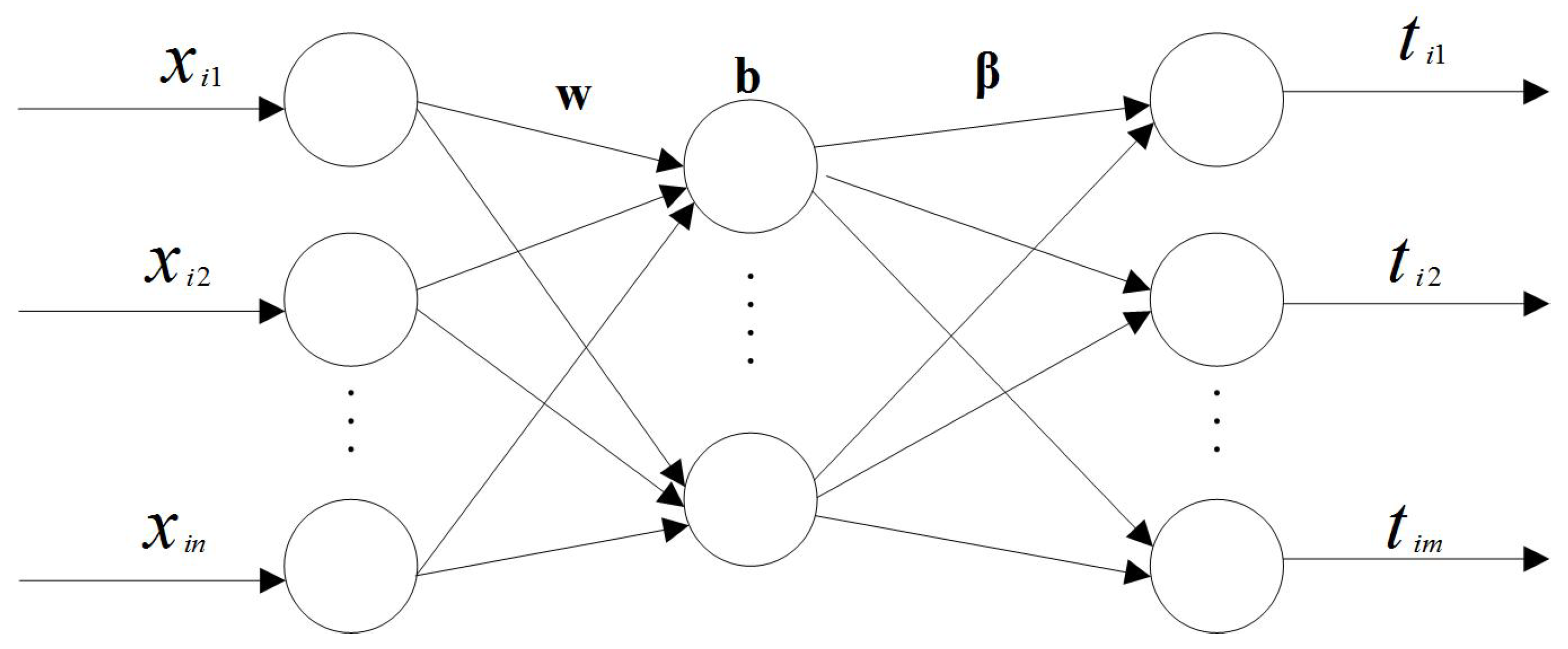
Extreme learning machine is a single hidden layer feedforward neural network. The input weights and biases are randomly generated, while the output weights can be automatically determined. Compared with the traditional methods such as BP neural network [39], the speed of ELM is faster [40,41]. The structure of ELM is shown in Figure 1.

For N arbitrary distinct samples, ${\left\{{\mathit{x}}_i,{\mathit{t}}_i\right\}}_{i=1}^N$, ${\mathit{x}}_i={\left[x_{i1},x_{i2},\cdots ,x_{in}\right]}^T\in {\mathbb{R}}^n,{\mathit{t}}_i={\left[t_{i1},t_{i2},\cdots ,t_{im}\right]}^T\in {\mathbb{R}}^m$. If the activation function is $g\left(\mathit{x}\right)$ with L hidden nodes, the output of ELM is as

$$\sum _{j=1}^L{\mathit{\beta }}_{j}g({\mathit{w}}_j·{\mathit{x}}_i+b_j)={\mathit{o}}_j,i=1,2,\cdots ,N$$

(1)

where ${\mathit{w}}_j={\left[w_{j1},w_{j2},\cdots ,w_{jn}\right]}^T$ is the weights connecting the jth hidden node with the input nodes, ${\mathit{\beta }}_j={\left[{\beta }_{j1},{\beta }_{j2},\cdots ,{\beta }_{jm}\right]}^T$ is the weights connecting the jth hidden node with the output nodes, $b_j$ is the bias of the jth hidden nodes. According to the theory [24], ELM can approximate these N samples with zero error and ${\sum }_{i=1}^N∥{\mathit{o}}_i-{\mathit{t}}_i∥=0$. Thus, the output of ELM can be expressed compactly as

$$\mathit{H}\mathit{\beta }=\mathit{T}$$

(2)

where $\mathit{H}$ is the output matrix of hidden layer and $\mathit{T}$ is the output matrix of output layer. They are as:

$$\mathit{H}={\left[\begin{array}{ccc}g({\mathit{w}}_1,{\mathit{b}}_1,{\mathit{x}}_1)& \cdots & g({\mathit{w}}_L,{\mathit{b}}_L,{\mathit{x}}_1)\\ ⋮& \ddots & ⋮\\ g({\mathit{w}}_1,{\mathit{b}}_1,{\mathit{x}}_N)& \cdots & g({\mathit{w}}_L,{\mathit{b}}_L,{\mathit{x}}_N)\end{array}\right]}_{N\times L}\mathrm{and}\mathit{T}={\left[\begin{array}{c}{\mathit{t}}_1^T\\ ⋮\\ {\mathit{t}}_N^T\end{array}\right]}_{N\times m}$$

(3)

The output weights matrix $\mathit{\beta }$ can be estimated as

$$\widehat{\mathit{\beta }}={\mathit{H}}^{†}\mathit{T}$$

(4)

where ${\mathit{H}}^{†}$ is the Moore–Penrose generalized inverse of the hidden layer output matrix $\mathit{H}$. It can be computed by orthogonal projection method, orthogonalization method and singular value composition (SVD) [42]. To improve the generalization performance of ELM, regularization is introduced and the optimization problem of ELM is as follows:

$$\begin{array}{c}\min \frac{1}{2}{∥\mathit{\beta }∥}^2+C\frac{1}{2}\sum _{i=1}^N∥{\mathit{\xi }}_i∥\hfill \\ s.t.h\left({\mathit{x}}_i\right)\mathit{\beta }={\mathit{t}}_i^T-{\mathit{\xi }}_i^{T}i=1,2,\cdots ,N\hfill \end{array}$$

(5)

where C is a penalty factor, and ${\mathit{\xi }}_i$ is the training error which is used to eliminate over-fitting. According to KKT conditions [26], if $L<N$, the $\mathit{\beta }$ is as

$$\mathit{\beta }={(\frac{\mathit{I}}{C}+{\mathit{H}}^T\mathit{H})}^{-1}{\mathit{H}}^T\mathit{T}$$

(6)

Thus, the output of ELM is as

$$f\left(\mathit{x}\right)=h\left(\mathit{x}\right)\mathit{\beta }=h\left(\mathit{x}\right){(\frac{\mathit{I}}{C}+{\mathit{H}}^T\mathit{H})}^{-1}{\mathit{H}}^T\mathit{T}$$

(7)

If $L\ge N$, the $\mathit{\beta }$ is as

$$\mathit{\beta }={\mathit{H}}^T{(\frac{\mathit{I}}{C}+\mathit{H}{\mathit{H}}^T)}^{-1}\mathit{T}$$

(8)

Thus, the final output of ELM is

$$f\left(\mathit{x}\right)=h\left(\mathit{x}\right)\mathit{\beta }=h\left(\mathit{x}\right){\mathit{H}}^T{(\frac{\mathit{I}}{C}+\mathit{H}{\mathit{H}}^T)}^{-1}\mathit{T}$$

(9)

The classification label of ELM is as

$$label\left(\mathit{x}\right)=\underset{i\in \left\{1,2,\cdots ,m\right\}}{\mathrm{argmax}}{f}_i\left(\mathit{x}\right)$$

(10)

where $f\left(\mathit{x}\right)=\left[f_1\left(\mathit{x}\right),f_2\left(\mathit{x}\right),\cdots ,f_m\left(\mathit{x}\right)\right]$.

From the above descriptions, the steps of ELM are summarized as follows (Algorithm 1) [24,25]:

Algorithm 1 ELM.

Input: a training data $\mathcal{X}=\left\{({\mathit{x}}_i,{\mathit{y}}_i)|{\mathit{x}}_i\in {\mathbb{R}}^n,{\mathit{y}}_i\in {\mathbb{R}}^m\right\}$; the number of hidden nodes L; the activation function $g(·)$; Output: ELM classifier.     Step 1: Randomly generate the input weights $w_j$ and biases ${\mathit{b}}_j,j=1,2,\cdots ,L;$     Step 2: Calculate the output matrix of hidden layer $\mathit{H}$ for dataset $\mathcal{X}$     Step 3: Obtain the output weights $\mathit{\beta }$ according to Equation (6) or Equation (8);

3. The Basic Principles of CELM

In this section, we introduce the dimension-reduction method which is used to reduce the dimension of the data at first, and then explain the details of concept drift detection mechanism and classification steps of CELM.

3.1. The Method of Dimensionality Reduction for Data Stream

Dimensionality reduction is important for data stream classification. It can reduce the dimension of the data and improve the efficiency of the algorithm. In this paper, LLE method [43] is used to handle data stream. Let a data block be ${\mathit{B}}_i=\left\{{\mathit{x}}_1,{\mathit{x}}_2,\cdots ,{\mathit{x}}_N\right\}$, for a data point ${\mathit{x}}_i,i=1,2,\cdots ,N$, LLE (https://cs.nyu.edu/~roweis/lle/) finds k neighborhood points of ${\mathit{x}}_i$ to reconstruct ${\mathit{x}}_i$. The objective function of the optimization problem is as follows:

$$\begin{array}{c}\min J\left(\mathit{w}\right)={\sum }_{i=1}^N{∥{\mathit{x}}_i-{\sum }_{j=1}^k{w}_{ij}{\mathit{x}}_j∥}_2^2\hfill \\ s.t.{\sum }_{j=1}^k{w}_{ij}=1\hfill \end{array}$$

(11)

where $w_{ij}$ is the weight of the neighborhood sample ${\mathit{x}}_j$. If ${\mathit{x}}_j$ is not the neighborhood of ${\mathit{x}}_i$, $w_{ij}=0$. From Equation (11), it follows:

$$\begin{array}{cc}\hfill J\left(\mathit{w}\right)& ={\sum }_{i=1}^N{∥1·{\mathit{x}}_i-{\sum }_{j=1}^k{w}_{ij}{\mathit{x}}_j∥}_2^2={\sum }_{i=1}^N{∥{\sum }_{j=1}^k{w}_{ij}{\mathit{x}}_i-{\sum }_{j=1}^k{w}_{ij}{\mathit{x}}_j∥}_2^2\hfill \\ & ={\sum }_{i=1}^N{∥{\sum }_{j=1}^k{w}_{ij}({\mathit{x}}_i-{\mathit{x}}_j)∥}_2^2={\sum }_{i=1}^N{∥({\mathit{x}}_i-{\mathit{x}}_j){\mathit{W}}_i∥}_2^2\hfill \\ & ={\sum }_{i=1}^N{\mathit{W}}_i^T{({\mathit{x}}_i-{\mathit{x}}_j)}^T({\mathit{x}}_i-{\mathit{x}}_j){\mathit{W}}_i\hfill \end{array}$$

(12)

where ${\mathit{W}}_i={\left[w_{i1},w_{i2},\cdots ,w_{ik}\right]}^T$. Let ${\mathit{Z}}_i={({\mathit{x}}_i-{\mathit{x}}_j)}^T({\mathit{x}}_i-{\mathit{x}}_j)$, so it will have

$$J\left(\mathit{w}\right)=\sum _{i=1}^N{\mathit{W}}_i^T{\mathit{Z}}_i{\mathit{W}}_i\mathrm{and}\sum _{j=1}^k{w}_{ij}={\mathit{W}}_i^T{\mathbf{1}}_k=1$$

(13)

where ${\mathbf{1}}_k$ is a vector in which all elements are 1. The optimization function of Equation (13) can be expressed as

$$L=\sum _{i=1}^N{\mathit{W}}_i^T{\mathit{Z}}_i{\mathit{W}}_i+\lambda ({\mathit{W}}_i^T{\mathbf{1}}_k-1)\Rightarrow \frac{\partial L}{\partial {\mathit{W}}_i}=2{\mathit{Z}}_i{\mathit{W}}_i+\lambda {\mathbf{1}}_k=0$$

(14)

From Equations (13) and (14), it will obtain

$${\mathit{W}}_i=\frac{{\mathit{Z}}_i^{-1}{\mathbf{1}}_k}{{\mathbf{1}}_k^T{\mathit{Z}}_i^{-1}{\mathbf{1}}_k}$$

(15)

For ${\mathit{B}}_i=\left\{{\mathit{x}}_1,{\mathit{x}}_2,\cdots ,{\mathit{x}}_N\right\}$, the projection of ${\mathit{B}}_i$ in low dimension space is $\left\{{\mathit{y}}_1,{\mathit{y}}_2,\cdots ,{\mathit{y}}_N\right\}$. The objection of dimension reduction is to make the following loss function is minimized.

$$\begin{array}{c}\min \sum _{i=1}^N{∥{\mathit{y}}_i-\sum _{j=1}^k{w}_{ij}{y}_j∥}_2^2\hfill \\ s.t.\sum _{i=1}^N{\mathit{y}}_i=0\mathrm{and}\frac{1}{N}\sum _{i=1}^N{\mathit{y}}_i{\mathit{y}}_i^T=\mathit{I}\hfill \end{array}$$

(16)

Equation (16) can be changed as

$$\begin{array}{cc}\hfill J\left(\mathit{Y}\right)& =\sum _{i=1}^N{∥{\mathit{y}}_i-\sum _{j=1}^k{w}_{ij}{y}_j∥}_2^2=\sum _{i=1}^N{∥\mathit{Y}{\mathit{I}}_i-\mathit{Y}{\mathit{W}}_i∥}_2^2\hfill \\ & =tr\left({\mathit{Y}}^T{(\mathit{I}-\mathit{W})}^T(\mathit{I}-\mathit{W})\mathit{Y}\right)\hfill \end{array}$$

(17)

Let $\mathit{M}={(\mathit{I}-\mathit{W})}^T(\mathit{I}-\mathit{W})$, so the objective function of the optimization problem is

$$\begin{array}{c}\min J\left(\mathit{Y}\right)=tr\left({\mathit{Y}}^T\mathit{M}\mathit{Y}\right)\hfill \\ s.t.{\mathit{Y}}^T\mathit{Y}=N\mathit{I}\hfill \end{array}$$

(18)

Construct the following Lagrange function

$$L\left(\mathit{Y}\right)=tr\left({\mathit{Y}}^T\mathit{M}\mathit{Y}\right)+\lambda ({\mathit{Y}}^T\mathit{Y}-N\mathit{I})$$

(19)

By solving the partial derivation of $L\left(\mathit{Y}\right)$, it will get

$$\frac{\partial L}{\partial \mathit{Y}}=\mathit{M}\mathit{Y}-\lambda \mathit{Y}=0\Rightarrow \mathit{M}\mathit{Y}=\lambda \mathit{Y}$$

(20)

Equation (20) means $\mathit{Y}$ is the eigenvectors of $\mathit{M}$. If it wants to get d-dimensional data, it only needs to find a matrix which is made up by $d+1$ eigenvectors corresponding to the least $d+1$ eigenvalues of the matrix $\mathit{M}$, and $\mathit{Y}=\left\{{\mathit{y}}_2,{\mathit{y}}_3,\cdots ,{\mathit{y}}_{d+1}\right\}$. The dimension-reduction algorithm of CELM is as follows (Algorithm 2).

Algorithm 2 Dimension-reduction of data stream.

Input: Data stream $\mathit{S}$, the size of data block ${\mathit{B}}_i$: winsize, k and d; Output: $\mathit{Y}=\left\{{\mathit{y}}_1,{\mathit{y}}_2,\cdots ,{\mathit{y}}_d\right\}$.     while $\mathit{S}\ne NULL$ do         Get a data block ${\mathit{B}}_j=\left\{{\mathit{x}}_1,{\mathit{x}}_2,\cdots ,{\mathit{x}}_N\right\}$ with N samples from sliding window;         Calculate ${\mathit{W}}_i,i=1,2,\cdots ,N$;         Calculate $\mathit{M}={(\mathit{I}-\mathit{W})}^T(\mathit{I}-\mathit{W})$;         Calculate d+1 eigenvectors of the matrix $\mathit{M}$;         Get the low dimensional matrix $\mathit{Y}$;

3.2. The Data Stream Classification and Concept Drift Detection of CELM

Data stream is different from the traditional static data, concept drift is often happened, so concept drift detection must be included in the training process. For a data block ${\mathit{B}}_i$, the error rate of classifiers is $p_i$ which is a random variable obeying the Bernoulli distribution, so the standard deviation is $s_i=\sqrt{\frac{p_i(1-p_i)}{i}}$ where i is the number of samples [44,45]. In this paper, CELM utilizes $p_i$ and $s_i$ to detect concept drift. The change of data stream is divided into three types: stable, error level and concept drift.

If $p_i+s_i\le p_{min}+2s_{min}$ and $p_i<\epsilon$, it suggests that the error rate of classifiers system is in a low level and the concept of data stream is stable where $\epsilon$ is a threshold. Thus, the classifiers are suitable for the classification task of the current data stream and they do not need to make any adjustment.

If $p_i+s_i\ge p_{min}+2s_{min}$ and $p_i<\epsilon$, it suggests that the error rate of classifiers system is still in a low level, but the performance of classifers has a big fluctuation, the classifiers will give a warning and CELM will use online sequence learning mechanism [30] to update each classifier. At the initial time, let the data block be ${\mathit{B}}_0={\left\{{\mathit{x}}_i,{\mathit{t}}_i\right\}}_{i=1}^{N_0}$, so the output matrix of hidden layer ${\mathit{H}}_0$ and the initial target matrix of ${\mathit{T}}_0$ are

$${\mathit{H}}_0={\left[\begin{array}{ccc}g({\mathit{w}}_1,b_1,{\mathit{x}}_1)& \cdots & g({\mathit{w}}_L,b_L,{\mathit{x}}_1)\\ ⋮& \ddots & ⋮\\ g({\mathit{w}}_1,b_1,{\mathit{x}}_{N_0})& \cdots & g({\mathit{w}}_L,b_L,{\mathit{x}}_{N_0})\end{array}\right]}_{N_0\times L}\mathrm{and}{\mathit{T}}_0={\left[\begin{array}{c}{\mathit{t}}_1^T\\ ⋮\\ {\mathit{t}}_{N_0}^T\end{array}\right]}_{N_0\times m}$$

(21)

The initial output weight of ELM ${\mathit{\beta }}^{\left(0\right)}$ is

$${\mathit{\beta }}^{\left(0\right)}={\mathit{K}}_0^{-1}{\mathit{H}}_0^T{\mathit{T}}_0$$

(22)

where ${\mathit{K}}_0=\frac{\mathit{I}}{C}+{\mathit{H}}^T\mathit{H}$ and ${\mathit{T}}_0={\left[{\mathit{t}}_1,{\mathit{t}}_2,\cdots ,{\mathit{t}}_{N_0}\right]}^T$. After (k + 1)th data block coming into sliding window, the data block is ${\mathit{B}}_{k+1}={\left\{{\mathit{x}}_i,{\mathit{t}}_i\right\}}_{i={\sum }_{j=0}^k{N}_j+1}^{{\sum }_{j=0}^{k+1}{N}_j}$. The output matrix of hidden layer ${\mathit{H}}_{k+1}$ is

$${\mathit{H}}_{k+1}={\left[\begin{array}{ccc}g({\mathit{w}}_1,b_1,{\mathit{x}}_{{\sum }_{j=0}^k{N}_j+1})& \cdots & g({\mathit{w}}_L,b_L,{\mathit{x}}_{{\sum }_{j=0}^k{N}_j+1})\\ ⋮& \ddots & ⋮\\ g({\mathit{w}}_1,b_1,{\mathit{x}}_{{\sum }_{j=0}^{k+1}{N}_j})& \cdots & g({\mathit{w}}_L,b_L,{\mathit{x}}_{{\sum }_{j=0}^{k+1}{N}_j})\end{array}\right]}_{N_{k+1}\times L}$$

(23)

$${\mathit{T}}_{k+1}={\left[{\mathit{t}}_{1+{\sum }_{j=0}^k{N}_j}^T,\cdots ,{\mathit{t}}_{{\sum }_{j=0}^{k+1}{N}_j}^T\right]}_{N_{k+1}\times m}^T$$

(24)

The ${\mathit{K}}_{k+1}$ and ${\mathit{\beta }}^{(k+1)}$ are updated as

$${\mathit{K}}_{k+1}={\mathit{K}}_k+{\mathit{H}}_{k+1}^T{\mathit{H}}_{k+1}$$

(25)

$${\mathit{\beta }}^{(k+1)}={\mathit{\beta }}^{\left(k\right)}+{\mathit{K}}_{k+1}^{-1}{\mathit{H}}_{k+1}^T({\mathit{T}}_{k+1}-{\mathit{H}}_{k+1}{\mathit{\beta }}^{\left(k\right)})$$

(26)

when calculating the output weight matrix $\mathit{\beta }$ , it needs to perform a matrix inversion, but the calculated amount of the pseudo inverse is very large, so Woodbury formula is often used to diminish the computation [37] and the formula is as

$$\begin{array}{cc}\hfill {\mathit{K}}_{k+1}^{-1}& ={({\mathit{K}}_k+{\mathit{H}}_{k+1}^T{\mathit{H}}_{k+1})}^{-1}\hfill \\ & ={\mathit{K}}_k^{-1}-{\mathit{K}}_k^{-1}{\mathit{H}}_{k+1}^T{(\mathit{I}+{\mathit{H}}_{k+1}{\mathit{K}}_k^{-1}{\mathit{H}}_{k+1}^T)}^{-1}{\mathit{H}}_{k+1}{\mathit{K}}_k^{-1}\hfill \end{array}$$

(27)

By the online sequential learning mechanism, when the change of concept in data stream is small, CELM can update classifiers to adapt to the change of concept which is also effective for gradual concept drift.

If $p_i+s_i\ge p_{min}+2s_{min}$ or $p_i\ge \epsilon$, it indicates that the change of data stream is too large or the performance of classifiers is in low level. The classification model is not fit for the current data stream, so all classifiers must be deleted and retrain a series of classifiers. The steps of CELM are summarized in Algorithm 3.

Algorithm 3 CELM.

Input: Data stream $\mathit{S}$, the size of data block ${\mathit{B}}_i$: winsize, k and d, $\epsilon$, K classifiers; Output: An ensemble classifiers system.     while $\mathit{S}\ne NULL$ do         Get a data ${\mathit{B}}_i$ from sliding window;         Use Algorithm 2 to descend dimension for ${\mathit{B}}_i$;         if $p_i+s_i<p_{min}+2s_{min}\&\&p_i<\epsilon$ then             The data stream is stable and directly uses classifier to finish classification task;         else if $p_i+s_i\ge p_{min}+2s_{min}\&\&p_i<\epsilon$ then             Uses online learning mechanism to update classifiers as Equations (21)–(27);         else if $p_i+s_i\ge p_{min}+2s_{min}\left|\right|p_i\ge \epsilon$ then             Concept drift has happened;             Delete all classifiers and retrain each classifier as Algorithm 1;

From the steps of CELM, it is known that, when the change of data stream is small, CELM uses online sequential learning mechanism to update classifiers which ensures the classifiers can utilize the last model and do not need to be retrained again and again; in other words, the method also gives a way to handle gradual concept drift. In addition, the dimension-reduction algorithm which preprocesses data blocks and the advantages of ELM makes CELM keep a good performance and have a fast speed.

4. Experiments and Data Analysis

In the section, experiments and data analysis are executed to test the performance of CELM. OS-ELM [30], SEA [46], AE [47] and M_ID4 [48] are used as comparison algorithms. All algorithms were executed on MATLAB 2017a platform, windows 7 OS, Intel quad-core 3.30 GHz CPU and 8 G memory. There are 10 artificial and real datasets for experimental datasets. The base classifier of SEA, AE and M_ID4 is decision tree and the number of sub-classifiers is set to 5. For CELM, the parameter C = 1000, the neighbourhood k = 5 and the threshold $\epsilon =0.3$. For M_ID4, the threshold $\theta =0.01$ and the decay factor b = 0.5. The activation function of CELM and OS-ELM is sigmoid.

4.1. Datasets

At first, we will give a brief introduction about datasets. All artificial datasets are generated from MOA platform [49]. In artificial datasets, we only give a explain about hyperplane dataset, the other description of datasets can be see from UCI website (http://archive.ics.uci.edu/ml/datasets.html) and help handbook. The basic information of datasets are shown in

Table 1. The information of the experimental datasets.

Dataset	Size	Attributes	Classes	Types
voice	7614	385	12	Numeric
waveform	50,000	21	3	Numeric
bank	45,211	16	2	Mixed
adult	32,561	13	2	Mixed
letter	20,000	16	26	Categorical
hyperplane	50,000	40	2	Numeric
occupancy	8143	5	2	Numeric
hill	1212	100	2	Numeric
Protein	1080	80	8	Mixed
Ozone	2534	72	2	Numeric

.

hyperplane is a gradual concept drift dataset. In a d-dimensional space, a hyperplane is defined as ${\sum }_{i=1}^d{w}_i{x}_i=w_0$, where $x_i\in \left[0,1\right]$, $w_i\in \left[-10,10\right]$ and $w_0=\frac{1}{2}{\sum }_{i=1}^d{w}_i$. If ${\sum }_{i=1}^d{w}_i{x}_i\ge w_0$, the point is remarked as positive; if ${\sum }_{i=1}^d{w}_i{x}_i<w_0$, the point is remarked as negative.

4.2. The Comparison Results of CELM and Comparison Algorithms on the Test Datasets

To test the performance of CELM and comparison algorithms, the algorithms are executed on 10 datasets. The test results are shown in

Table 2. The test accuracies of the algorithms on the experimental datasets.

Dataset	CELM	SEA	AE	OS-ELM	M_ID4	winsize	d	L
voice	0.6511 ± 0.1786	0.3357 ± 0.0651	0.4155 ± 0.0737	0.2808 ± 0.0429	0.6029 ± 0.1033	100	5	20
waveform	0.6619 ± 0.0119	0.6329 ± 0.0136	0.6374 ± 0.0204	0.6856 ± 0.0134	0.6205 ± 0.0195	1000	200	200
bank	0.8863 ± 0.0094	0.8841 ± 0.0088	0.8843 ± 0.0084	0.8812 ± 0.0087	0.8269 ± 0.0196	1200	13	5
adult	0.7596 ± 0.0135	0.8119 ± 0.0168	0.8156 ± 0.0117	0.7569 ± 0.0177	0.7501 ± 0.0235	1000	5	5
letter	0.4930 ± 0.0581	0.0361 ± 0.0096	0.3617 ± 0.0597	0.0418 ± 0.0046	0.6818 ± 0.1368	1000	13	2000
hyperplane	0.5812 ± 0.0205	0.5761 ± 0.0164	0.5758 ± 0.0182	0.5796 ± 0.0306	0.5385 ± 0.0199	1000	30	2000
occupancy	0.9670 ± 0.0294	0.9882 ± 0.0111	0.9788 ± 0.0191	0.7835 ± 0.0291	0.9640 ± 0.0182	100	5	10
hill	0.5517 ± 0.0659	0.5643 ± 0.0813	0.4833 ± 0.0491	0.4900 ± 0.0344	0.5283 ± 0.0369	60	80	100
Protein	0.6354 ± 0.0599	0.5750 ± 0.1578	0.6583 ± 0.1532	0.1354 ± 0.0348	0.5854 ± 0.1125	80	50	1000
Ozone	0.9408 ± 0.0107	0.9396 ± 0.0251	0.9392 ± 0.0131	0.9408 ± 0.0107	0.7692 ± 0.1018	120	30	200
Average	0.7128 ± 0.0297	0.6344 ± 0.0406	0.6750 ± 0.0424	0.5576 ± 0.0227	0.6868 ± 0.0592	–	–	–

and

Table 3. The time consumption of the algorithms on the experimental datasets.

Dataset	CELM	SEA	AE	OS-ELM	M_ID4
voice	2.0433	2401.3555	291.9706	0.1160	5234.9994
waveform	82.9626	1523.1448	172.0207	0.1480	>20,000
bank	10.8994	573.6019	63.8236	0.1100	2392.9633
adult	6.1201	279.0587	37.7094	0.0566	2830.5794
letter	70.0543	248.7848	29.8872	0.0865	3638.3141
hyperplane	27.5537	1558.7989	160.4245	0.2402	3486.1807
occupancy	1.2085	15.4485	2.3894	0.0632	75.3053
hill	0.5319	59.4144	8.9018	0.0548	75.0302
Protein	4.2500	40.2288	6.3598	0.0426	14.2372
Ozone	0.4528	64.5923	6.0510	0.0739	32.7597

.

Table 2 and Table 3 show that CELM gets best results on four datasets; SEA, AE and OS-ELM get the best results on two datasets; and M_ID4 gets only one best result. In addition, the average accuracy of CELM is also the best of all. For time consumption, OS-ELM is the least of all and CELM the second least, but the accuracies of CELM are much higher than OS-ELM. Thus, it can be concluded that the performance of CELM is better than the other algorithm in most conditions. On Ozone dataset, CELM and OS-ELM get the same highest accuracy because Ozone has no abrupt concept drift and CELM degenerates into OS-ELM; in other words, there will be no difference between CELM and OS-ELM when dataset has no abrupt concept drift.

4.3. The Effect of Sliding Window on the Performance of CELM

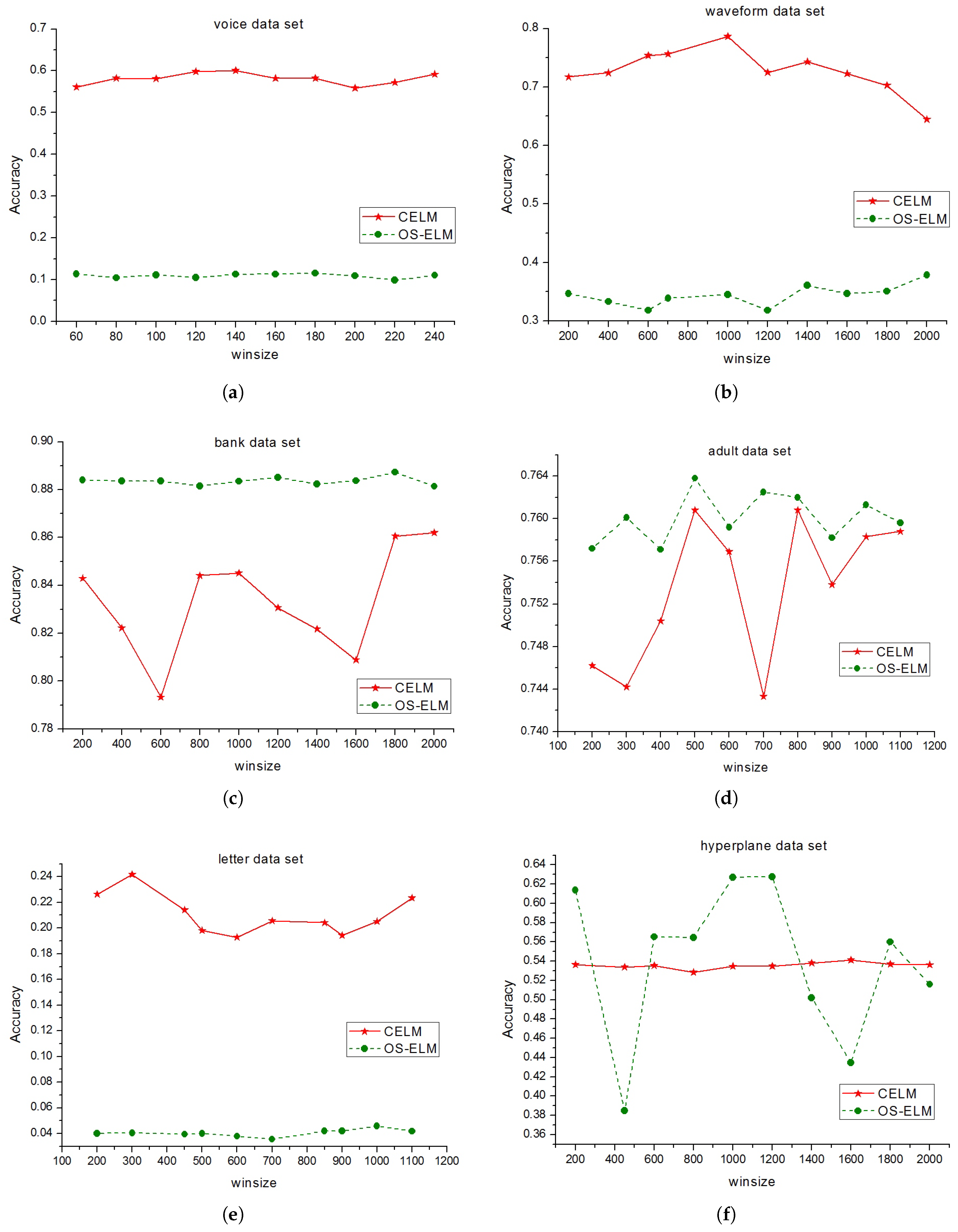
To test the effect of sliding window on the performance of CELM, this paper chooses different winsize values, and executes CELM and OS-ELM on the experimental datasets. The number of hidden nodes is 20 and d = 5. The test results are shown in Figure 2a–j.

In Figure 2a–j, the accuracies of CELM and OS-ELM are changing with different winsize values. On the voice, waveform, letter, occupancy and protein datasets, CELM is much better than OS-ELM; the classification performance of OS-ELM is at a low level because there are many abrupt concept drifts in those datasets. It suggests that OS-ELM is not fit for dealing with data stream with abrupt concept drift and CELM has an obvious advantage in handling data stream with abrupt concept drift. On the other datasets, the test results of OS-ELM is better than that of CELM. If analyzing the change of the curve, it is known that there is no big difference between OS-ELM and CELM in accuracy and both get good results because the change of concepts in those dataset is small. Therefore, it can be concluded that CELM can cope with gradual concept drift and abrupt concept drift, but OS-ELM can only face gradual concept drift; thus, CELM is better than OS-ELM.

4.4. The Effect of the Values of d on the Performance of CELM

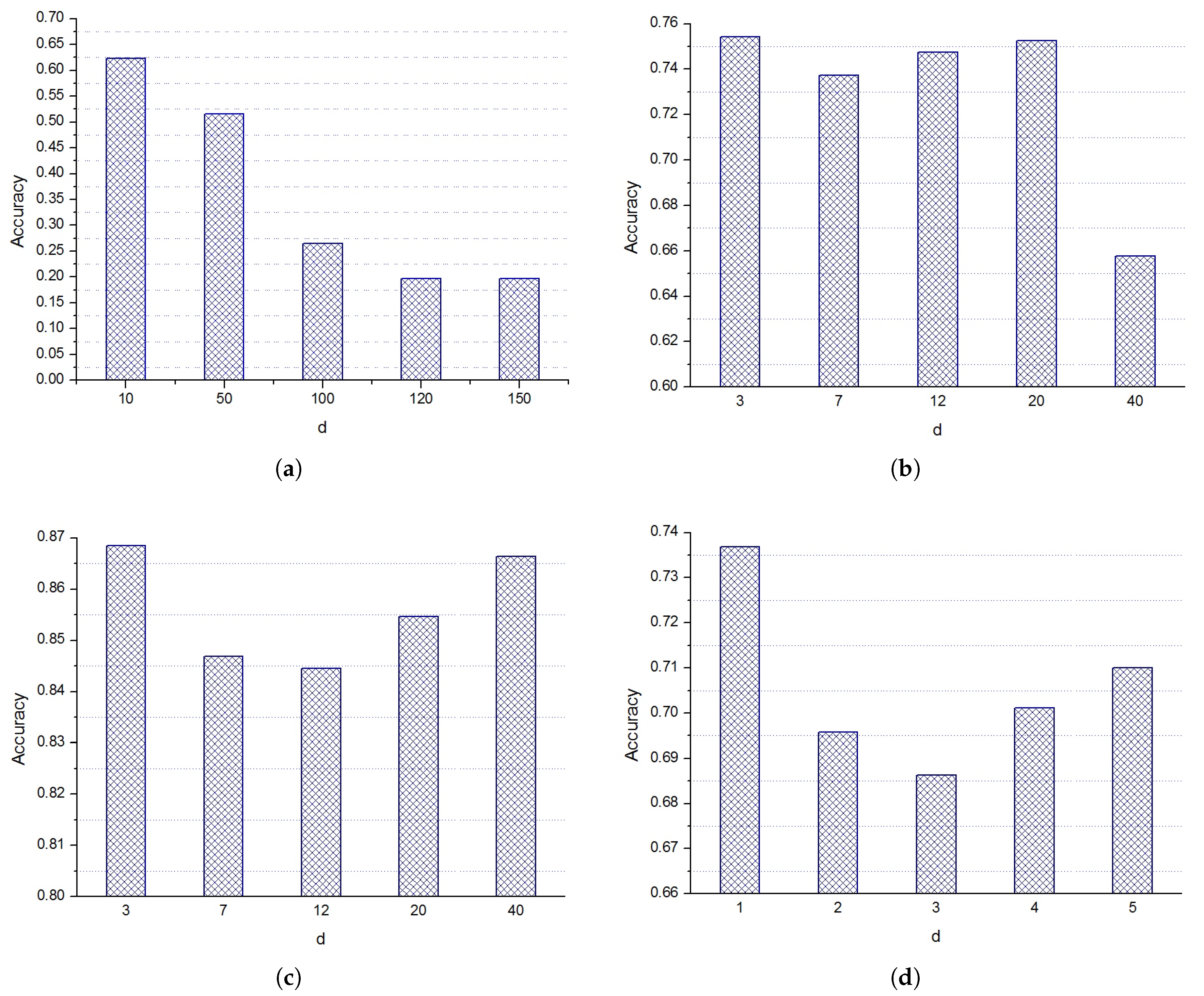
To test the effect of d on the performance of CELM, this paper executes CELM with different values of k which is a parameter of Algorithm 2. The activation function of CELM is sigmoid; the size of sliding window is 90; and the number of hidden nodes is 30.

Table 4. The dimension reduction result of CELM testing in Table 2.

Dataset	The Number of Original Features	After Dimension Reduction	Decrement	Reduction Rate
voice	385	5	380	0.9870
adult	13	5	7	0.5384
letter	16	13	3	0.1875
hyperplane	40	30	10	0.2500
occupancy	5	5	0	0.0000
hill	100	80	20	0.2000
Protein	80	50	30	0.3750
Ozone	72	30	42	0.5833

is the dimension decrement of the datasets testing on CELM. From the result analysis of Table 2, it can be known that the performance of CELM is the best. CELM reduces the dimensions of most datasets. In other words, the dimensionality reduction methods of manifold learning in CELM is effective. Figure 3 presents the result of CELM testing on the experimental datasets with different d values. d is an important parameter for the dimension reduction algorithm which is presented as Algorithm 2. Data will lose more information if d is a small value and data will have many redundant features if d is a larger value. It is known that the performance of CELM will change when d value changes. The accuracy of CELM has a large fluctuation on voice, waveform, adult, letter, occupancy, hill and protein datasets and the accuracy of CELM has less fluctuation on the other datasets, as shown in Figure 2 and

Table 5. The accuracy standard deviation of CELM testing in Figure 3.

Dataset	Voice	Waveform	Bank	Adult	Letter	Hyperplane	Occupancy	Hill	Protein	Ozone
Standard deviation	0.1971	0.0409	0.0109	0.0193	0.0816	0.0112	0.0373	0.0222	0.1992	0.0045

. It manifests d values can affect the effect of dimensionality reduction algorithm. In addition, it is obvious that the performance of CELM will be affected if the value of d is too large or too small, therefore the user needs to select a appropriate value for the manifold learning algorithm.

5. Conclusions

Data stream classification is a hot research topic in recent years. How to deal with the data stream with concept drift has a high value of practical application. A new ensemble extreme learning machine with concept drift detection (CELM) is presented in this paper. CELM applies manifold learning method to reduce the dimensions of data blocks and divides the changes of concepts in data stream into three types: stable, warning and concept drift. The algorithm can detect both gradual concept drift and abrupt concept drift by online sequential learning and concept drift detection mechanisms which expands the application scope of ELM. The experimental results also prove that the proposed algorithm is effective for data stream classification.

It is obvious that this algorithm still has some problems to be solved. The number of hidden nodes L and the parameter of the manifold learning algorithm d have a great impact on CELM. How to select appropriate values for those parameters will be a research direction for future works.

References

- Gedik, B.; Schneider, S.; Hirzel, M.; Wu, K.L. Elastic Scaling for Data Stream Processing. IEEE Trans. Parallel Distrib. Syst. 2014, 25, 1447–1463. [Google Scholar] [CrossRef] [Green Version]
- Krempl, G.; Last, M.; Lemaire, V.; Noack, T.; Shaker, A.; Sievi, S.; Spiliopoulou, M. Open challenges for data stream mining research. ACM SIGKDD Explor. Newsl. 2014, 16, 1–10. [Google Scholar] [CrossRef] [Green Version]
- Xu, S.; Wang, J. Classification Algorithm Combined with Unsupervised Learning for Data Stream. Pattern Recognit. Artif. Intell. 2016, 29, 665–672. [Google Scholar]
- Ramirez-Gallego, S.; Krawczyk, B.; Garcia, S.; Woźniak, M.; Herrera, F. A survey on data preprocessing for data stream mining: Current status and future directions. Neurocomputing 2017, 239, 39–57. [Google Scholar] [CrossRef]
- Sun, D.; Zhang, G.; Yang, S.; Zheng, W.; Khan, S.U.; Li, K. Re-Stream: Real-time and energy-efficient resource scheduling in big data stream computing environments. Inf. Sci. 2015, 319, 92–112. [Google Scholar] [CrossRef] [Green Version]
- Xu, S.; Wang, J. Dynamic extreme learning machine for data stream classification. Neurocomputing 2017, 238, 433–449. [Google Scholar] [CrossRef]
- Puthal, D.; Nepal, S.; Ranjan, R.; Chen, J. DLSeF: A Dynamic Key-Length-Based Efficient Real-Time Security Verification Model for Big Data Stream. ACM Trans. Embed. Comput. Syst. 2017, 16, 51. [Google Scholar] [CrossRef]
- Pan, S.; Wu, K.; Zhang, Y.; Li, X. Classifier ensemble for uncertain data stream classification. In Proceedings of the Pacific-Asia Conference on Advances in Knowledge Discovery and Data Mining, Hyderabat, India, 21–24 June 2010; pp. 488–495. [Google Scholar]
- Xu, S.; Wang, J. A Fast Incremental Extreme Learning Machine Algorithm for Data Streams Classification. Expert Syst. Appl. 2016, 65, 332–344. [Google Scholar] [CrossRef]
- Brzezinski, D.; Stefanowski, J. Combining block-based and online methods in learning ensembles from concept drifting data streams. Inf. Sci. 2014, 265, 50–67. [Google Scholar] [CrossRef]
- Farid, D.M.; Li, Z.; Hossain, A.; Rahman, C.M.; Strachan, R.; Sexton, G.; Dahal, K. An adaptive ensemble classifier for mining concept drifting data streams. Expert Syst. Appl. 2013, 40, 5895–5906. [Google Scholar] [CrossRef] [Green Version]
- Bifet, A. Adaptive learning from evolving data streams. In International Symposium on Intelligent Data Analysis: Advances in Intelligent Data Analysis VIII; Springer: Berlin/Heidelberg, Germany, 2009; pp. 249–260. [Google Scholar]
- Schmidt, J.P.; Siegel, A.; Srinivasan, A. Chernoff-Hoeffding Bounds for Applications with Limited Independence. SIAM J. Discret. Math. 1995, 8, 223–250. [Google Scholar] [CrossRef]
- Xu, S.; Wang, J. Data Stream Classification Algorithm Based on Kappa Coefficient. Comput. Sci. 2016, 43, 173–178. [Google Scholar]
- Domingos, P.M.; Hulten, G. Mining high-speed data streams. In Proceedings of the Sixth ACM SIGKDD International Conference on Knowledge Discovery and Data Mining, Boston, MA, USA, 20–23 August 2000; pp. 71–80. [Google Scholar]
- Hulten, G.; Spencer, L.; Domingos, P.M. Mining time-changing data streams. In Proceedings of the Seventh ACM SIGKDD International Conference on Knowledge Discovery and Data Mining, San Francisco, CA, USA, 26–29 August 2001; pp. 97–106. [Google Scholar]
- Wu, X.; Li, P.; Hu, X. Learning from concept drifting data streams with unlabeled data. Neurocomputing 2012, 92, 145–155. [Google Scholar] [CrossRef]
- Li, P.; Wu, X.; Hu, X.; Wang, H. Learning concept-drifting data streams with random ensemble decision trees. Neurocomputing 2015, 166, 68–83. [Google Scholar] [CrossRef]
- Brzezinski, D.; Stefanowski, J. Prequential AUC for classifier evaluation and drift detection in evolving data streams. In Proceedings of the 3rd International Conference on New Frontiers in Mining Complex Patterns (NFMCP’14), Nancy, France, 19 September 2014; pp. 87–101. [Google Scholar]
- Rutkowski, L.; Pietruczuk, L.; Duda, P.; Jaworski, M. Decision Trees for Mining Data Streams Based on the McDiarmid’s Bound. IEEE Trans. Knowl. Data Eng. 2013, 25, 1272–1279. [Google Scholar] [CrossRef]
- Ghazikhani, A.; Monsefi, R.; Yazdi, H.S. Online neural network model for non-stationary and imbalanced data stream classification. Int. J. Mach. Learn. Cybern. 2014, 5, 51–62. [Google Scholar] [CrossRef]
- Jain, V. Perspective analysis of telecommunication fraud detection using data stream analytics and neural network classification based data mining. Int. J. Inf. Technol. 2017, 9, 303–310. [Google Scholar] [CrossRef]
- Gao, M.; Yang, X.; Jain, R.; Ooi, B.C. Spatio-temporal event stream processing in multimedia communication systems. In Proceedings of the Scientific and Statistical Database Management, International Conference (SSDBM), Heidelberg, Germany, 30 June– 2 July 2010; pp. 602–620. [Google Scholar]
- Huang, G.B.; Zhu, Q.Y.; Siew, C.K. Extreme learning machine: Theory and applications. Neurocomputing 2006, 70, 489–501. [Google Scholar] [CrossRef] [Green Version]
- Huang, G.B.; Zhou, H.; Ding, X.; Zhang, R. Extreme learning machine for regression and multiclass classification. IEEE Trans. Syst. Man Cybern. B 2012, 42, 513–529. [Google Scholar] [CrossRef] [PubMed]
- Huang, G.B.; Zhu, Q.Y.; Siew, C.K. Extreme learning machine: A new learning scheme of feedforward neural networks. In Proceedings of the 2004 IEEE International Joint Conference on Neural Networks (IEEE Cat. No. 04CH37541), Budapest, Hungary, 25–29 July 2004; Volume 2, pp. 985–990. [Google Scholar]
- Lu, S.; Qiu, X.; Shi, J.; Li, N.; Lu, Z.H.; Chen, P.; Yang, M.M.; Liu, F.Y.; Jia, W.J.; Zhang, Y. A Pathological Brain Detection System based on Extreme Learning Machine Optimized by Bat Algorithm. CNS Neurol. Disord.-Drug Target 2017, 16, 23–29. [Google Scholar] [CrossRef] [PubMed]
- Wang, S.H.; Muhammad, K.; Phillips, P.; Dong, Z.; Zhang, Y.D. Ductal carcinoma in situ detection in breast thermography by extreme learning machine and combination of statistical measure and fractal dimension. J. Ambient Intell. Humaniz. Comput. 2017, 1–11. [Google Scholar] [CrossRef]
- Wang, Y.; Cao, F.; Yuan, Y. A study on effectiveness of extreme learning machine. Neurocomputing 2014, 74, 2483–2490. [Google Scholar] [CrossRef]
- Liang, N.Y.; Huang, G.B.; Saratchandran, P.; Sundararajan, N. A fast and accurate online sequential learning algorithm for feedforward networks. IEEE Trans. Neural Netw. 2006, 17, 1411–1423. [Google Scholar] [CrossRef] [PubMed]
- Gu, Y.; Liu, J.; Chen, Y.; Jiang, X.; Yu, H. TOSELM: Timeliness Online Sequential Extreme Learning Machine. Neurocomputing 2014, 128, 119–127. [Google Scholar] [CrossRef]
- Shao, Z.; Meng, J.E. An online sequential learning algorithm for regularized Extreme Learning Machine. Neurocomputing 2016, 173, 778–788. [Google Scholar] [CrossRef]
- Yangjun, R.; Xiaoguang, S.; Huyuan, S.; Lijuan, S.; Xin, W. Boosting ridge extreme learning machine. In Proceedings of the 2012 IEEE Symposium on Robotics and Applications (ISRA), Kuala Lumpur, Malaysia, 3–5 June 2012; pp. 881–884. [Google Scholar]
- Zhao, J.; Wang, Z.; Dong, S.P. Online sequential extreme learning machine with forgetting mechanism. Neurocomputing 2012, 87, 79–89. [Google Scholar] [CrossRef]
- Mirza, B.; Lin, Z.; Liu, N. Ensemble of subset online sequential extreme learning machine for class imbalance and concept drift. Neurocomputing 2015, 149, 316–329. [Google Scholar] [CrossRef]
- Vanli, N.D.; Sayin, M.O.; Delibalta, I.; Kozat, S.S. Sequential Nonlinear Learning for Distributed Multiagent Systems via Extreme Learning Machines. IEEE Trans. Neural Netw. Learn. Syst. 2016, 28, 546–558. [Google Scholar] [CrossRef] [PubMed]
- Singh, R.; Kumar, H.; Singla, R.K. An intrusion detection system using network traffic profiling and online sequential extreme learning machine. Expert Syst. Appl. 2015, 42, 8609–8624. [Google Scholar] [CrossRef]
- Wang, H.; Fan, W.; Yu, P.S.; Han, J. Mining concept-drifting data streams using ensemble classifiers. In Proceedings of the Ninth ACM SIGKDD International Conference on Knowledge Discovery and Data Mining, Washingto, DC, USA, 24–27 August 2003; pp. 226–235. [Google Scholar]
- Han, J.; Kamber, M.; Pei, J. Data Mining: Concepts and Techniques; Morgan Kaufmann: Burlington, MA, USA, 2012. [Google Scholar]
- Feng, L.; Xu, S.; Wang, F.; Liu, S. Rough extreme learning machine: A new classification method based on uncertainty measure. arXiv, 2017; arXiv:1710.10824. [Google Scholar]
- Wang, J.; Xu, S.; Duan, B.; Liu, C.; Liang, J. An Ensemble Classification Algorithm Based on Information Entropy for Data Streams. arXiv, 2017; arXiv:1708.03496. [Google Scholar]
- Zhang, X. Matrix Analysis and Application, 2nd ed.; Tsinghua University Press: Beijing, China, 2013. [Google Scholar]
- Roweis, S.T.; Saul, L.K. Nonlinear Dimensionality Reduction by Locally Linear Embedding. Science 2000, 290, 2323–2326. [Google Scholar] [CrossRef] [PubMed] [Green Version]
- Gama, J.; Medas, P.; Castillo, G.; Rodrigues, P. Learning with Drift Detection. In Advances in Artificial Intelligence—Sbia 2004, Proceedings of the Brazilian Symposium on Artificial Intelligence, Sao Luis, Maranhao, Brazil, 29 September–1 October 2004; Springer: Berlin/Heidelberg, Germany, 2004; pp. 286–295. [Google Scholar]
- Gama, J.; Castillo, G. Learning with local drift detection. In Proceedings of the International Conference on Advanced Data Mining and Applications, Xi’an, China, 14–16 August 2006; pp. 42–55. [Google Scholar]
- Street, W.N.; Kim, Y. A streaming ensemble algorithm (SEA) for large-scale classification. In Proceedings of the Seventh ACM SIGKDD International Conference on Knowledge Discovery and Data Mining, San Francisco, CA, USA; 2001; pp. 377–382. [Google Scholar] [Green Version]
- Zhang, P.; Zhu, X.; Shi, Y.; Wu, X. An aggregate ensemble for mining concept drifting data streams with noise. In Proceedings of the 13th Pacific-Asia Conference on Advances in Knowledge Discovery and Data Mining (PAKDD ’09), Bangkok, Thailand, 27–30 April 2009; pp. 1021–1029. [Google Scholar]
- Sun, Y.; Mao, G.J.; Liu, X.; Liu, C.N. Mining Concept Drifts from Data Streams Based on Multi-classifiers. Acta Autom. Sin. 2008, 34, 2323–2326. [Google Scholar] [CrossRef]
- Bifet, A.; Holmes, G.; Kirkby, R.; Pfahringer, B. MOA: Massive Online Analysis. J. Mach. Learn. Res. 2010, 11, 1601–1604. [Google Scholar]
Figure 1.
The structure of ELM.
Figure 2.
The test result of CELM and OS-ELM with different winsize values.
Figure 3.
The test result CELM with different d values: (a) voice dataset; (b) waveform dataset; (c) bank dataset; (d) adult dataset; (e) letter dataset; (f) hyperplane dataset; (g) occupancy dataset; (h) hill dataset; (i) protein dataset; and (j) ozone dataset.