A Regional Topic Model Using Hybrid Stochastic Variational Gibbs Sampling for Real-Time Video Mining

Abstract

The events location and real-time computational performance of crowd scenes continuously challenge the field of video mining. In this paper, we address these two problems based on a regional topic model. In the process of video topic modeling, region topic model can simultaneously cluster motion words of video into motion topics, and the locations of motion into motion regions, where each motion topic associates with its region. Meanwhile, a hybrid stochastic variational Gibbs sampling algorithm is developed for inference of our region topic model, which has the ability of inferring in real time with massive video stream dataset. We evaluate our method on simulate and real datasets. The comparison with the Gibbs sampling algorithm shows the superiorities of proposed model and its online inference algorithm in terms of anomaly detection.

1. Introduction

Video mining is a hot topic that has attracted significant interests in recent years. Video mining is able to find the implicit, valuable, and understandable video patterns by analyzing visual features, time structure, event relationships, and semantic information of video data [1], which can be classified into video structure mining and video motion mining [2]. In particular, for poor structural videos such as traffic surveillance video, video motion mining can realize the applications of abnormal events detection or congestion analysis, and so on.

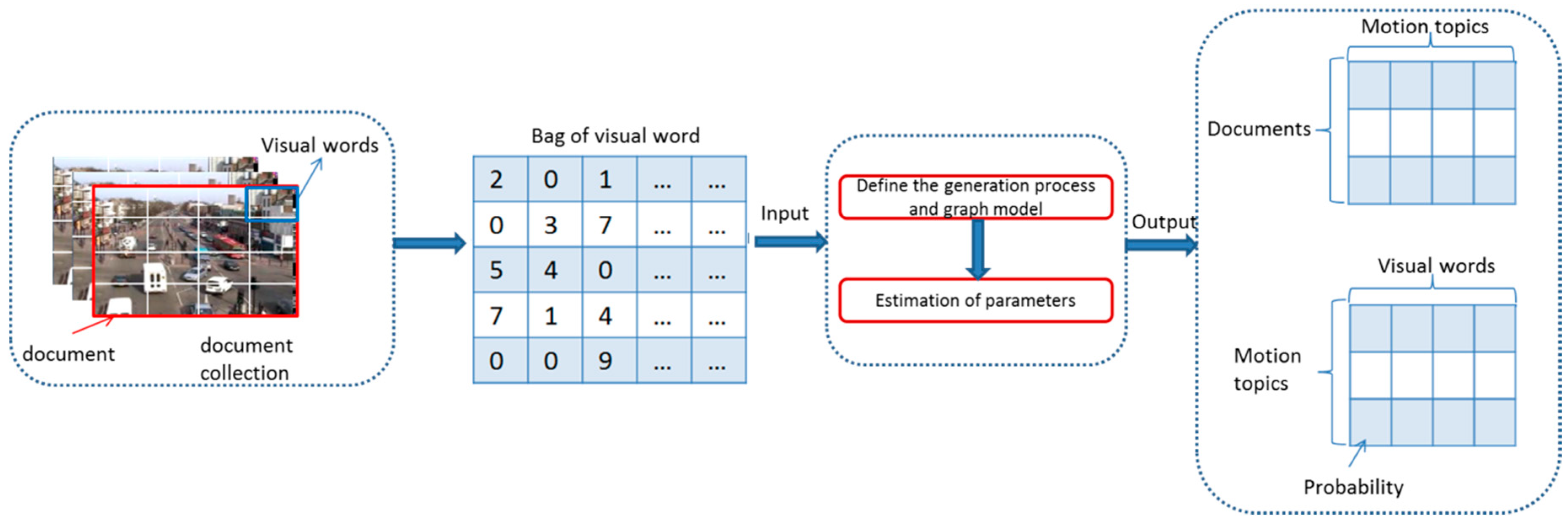
With the evolution of video mining technology, there has been an increasing number of research works focused on the use of topic models for video motion mining. Although probabilistic topic models were originally studied in the field of natural language processing [3,4], they also provide a way for discovering hidden pattern from images or document corpus. In the text mining, a topic model represents unlabeled documents as mixtures of topics where latent topics are distributions over observed words. In the video motion mining, full video is treated as document collection; a short video clip is treated as a document that divided from full video; the video features are considered as words. In this way, with the introduction of probabilitics topic model in video motion analysis, variety of latent motion patterns, and latent motions correlations were discovered, which are represented by topics. Figure 1 shows the diagram of video topic modeling.

Although several topic models have successfully applied in surveillance systems [5,6,7,8], there exist several premature phenomena in the procedure of video topic modeling—such as abnormal events locating and computational performance of real-time mining. In this paper, we focus on topic modeling with region information and uses it to automatically detect abnormal events from a complex video scene in real-time.

The rest of the paper is organized as follows. In the next section, we present a brief survey of the related works. In Section 3.1—Video Representation—the video representation is explained. In Section 3.2—Regional Topic Model and its Online Inference Algorithm, our regional topic model (RTM) and its hybrid stochastic variational Gibbs Sampling algorithm (HSVG) are presented. The datasets, evaluations and comparisons are discussed in detail, in Section 4. Our conclusions are presented in the last section.

2. Related Works

Recently, there has been a significant number of research works focused on the use of topic models for complex scene analysis. These methods have become quite popular due to their success in natural language processing, e.g., probabilistic latent semantic analysis (pLSA) [9] and latent Dirichlet allocation (LDA) [5]. Nevertheless, when there are lots of motions co-occurred, LDA has problems of low sensitivity, so it is unable to detect the abnormal event accurately. In addition, there is a problem with abnormal event localization in LDA: it can only detect which clip the abnormal event is in, but have no ability to determine where the event happened in. Therefore, several attempts have been made to model video data using LDA extensions.

X. Wang [10] adopted hierarchical variants of LDA, including a Hierarchical Dirichlet Processes (HDP) [7] mixture model and a Dual Hierarchical Dirichlet Processes (Dual-HDP) model, to connect three elements in visual surveillance: low-level visual features, simple atomic activities, and interactions. Thereafter, X. Wang [11] converted tracks into words, and applied a topic model to them. The words were the quantized positions and directions of motion, consequentially the topics would represent routes shared between objects. J. Li [12] proposed WS-JTM to address the typical topic model weakness of inference speed and exploited weak supervision. They fixed delta latent Dirichlet allocation (dLDA) in their extension, multi-class dLDA, which is also used to detect rare and subtle behavior. Thereafter, a two-staged cascaded LDA model was formulated by Li et al. in reference [13] where the first stage learns regional behavior and the second stage learns the global context over the regional models. Hospedales T.M. et al. [14] adopt a nonparametric Bayesian approach to automatically determine the number of topics shared by the documents and also when they appear in each temporal document. Emonet R. [15] proposed framework consists of an activity-based semantic scene segmentation model for learning behavior spatial context, and a cascaded probabilistic topic model for learning both behavior correlation context and behavior temporal context at multiple scales. Fu et al. [16] improved sparse topical coding (STC) to discover semantic motion patterns for a dynamic scene, which can be sparsely reconstructed. Yuan et al. [17] used a topic model to discover functional regions in a city using taxi probe data and point-of-interest information. Similarly, Farrahi and Gatica-Perez [18] used a topic model to discover human routines using mobile-phone location data. In [19], LDA was extended to model the flow of people entering or exiting a building. Yu et al. [20] proposed a topic model for detecting an anomalous group of individuals in a social network. Kinoshita et al. [21] introduced a traffic state model based on a probabilistic topic model to describe the traffic states for a variety of roads, the model can be learned using an expectation–maximization algorithm. Hospedales et al. [22] introduced a dynamic topic model named Markov clustering topic model (MCTM), and an approximation to online Bayesian inference was formulated to enable dynamic scene understanding and behavior mining in new video data online in real-time. In order to handle the temporal nature of the video data, Fan et al. [23] devised a dynamical causal topic model (DCTM) that can detect the latent topics and causal interactions between them.

Meanwhile, several attempts have also been made to find anomalies using topic models and surveillance cameras [24,25]. Jeong et al. [26] proposed a topic model for detecting anomalous trajectories of people or vehicles in surveillance-video images. Kaviani et al. [27] addressed the problem of abnormality detection based on a fully sparse topic models (FSTM). Isupova et al. [28] proposed a novel dynamic Bayesian nonparametric topic model and its Batch and online Gibbs samplers for anomaly detection in video.

In general, there were several key problems in existing studies about video mining using topic model: (1) model parameters increment leads to the increments of the model learning time, and then traditional off-line inference algorithm is not suitable for video monitoring system; (2) anomaly detection in a whole scene rather than in each region reduces the sensitivity of the anomaly detection.

To address the problem of motion region, Zou et al. [29] proposed a belief based on correlated topic model (BCTM) for the semantic region analysis of pedestrian motion patterns in the crowded scenes. Haines proposed regional LDA model (rLDA) [30], which not only can model activities in a complicated scene, but also realize a high sensitivity detection and the localization of motion topic (especially the abnormal event) by extracting spatial information ignored by LDA. Nonetheless, the inference algorithm of above studies still used the collapsed Gibbs sampling, which needs to scan the whole samples at each iteration. For huge data sets and data streams such as video, this way adopted by Gibbs sampling leads to high memory overhead, slow running speed, and judging convergence difficultly.

Classic approaches of inference algorithm in LDA are Gibbs sampling (GS) [31] and variational Bayesian (VB) batch inference [5]. In order to solve the problem of computational complexity, collapsed Gibbs sampling (CGS) [6] and collapsed VB batch inference (CVB) [32] were proposed. Nevertheless, for the purpose of LDA applied to video mining, we need to make the inference algorithm adapt to the characteristics of video streaming data set, it is better to a realize real-time and online processing quickly and efficiently. For text database which is huge or in the form of data stream, there have been developments of online LDA inference algorithm with less memory, faster running, and convergence speed. Hoffman proposed the stochastic gradient optimization algorithm (online LDA) [33], which repeatedly subsamples a small set of documents from the collection and then updates the topics from an analysis of the subsample. Since online LDA does not need to scan the entire samples for updating topic parameter matrix at each iteration, the updating of topic parameters is more frequently. The algorithm not only takes up less memory, faster running, and convergence speed, but also realizes online inference in real time for huge data sets or data stream. Nonetheless, the algorithm complexity linearly increased with the number of topics. Therefore, it is not suitable for large collection with many topics. On the basis of online LDA algorithm, Mimno proposed hybrid stochastic variational Gibbs sampling (HSVG) [34]. This algorithm introduced the second source of stochasticity by MCMC sampling, and taken advantage of sparse computation to make complexity sublinearly increased with the number of topics. It fits for a large collection with many topics. Besides, RLD (Riemannian Langevin dynamics) [35] algorithm was proposed by Girolami. It is a kind of Langevin dynamics algorithm based on Riemannian manifold of MH correction. Welling proposed SGLD (stochastic gradient Langevin dynamics) [36] algorithm, which reserved stochastic gradient optimization algorithm, and can sample from the posterior distribution. Patterson proposed SGRLD (stochastic gradient Riemannian Langevin dynamics) [37] by combining RLD and SGLD algorithm. In addition, Olga Isupova et al. [38] proposed new learning algorithms for activity analysis in video, which are based on the expectation maximization approach and variational Bayes inference.

3. Materials and Methods

3.1. Video Representation

To discover motion patterns for video by topic modeling, the definitions of visual words and visual documents are essential for topic model applied to video analysis: given an input video, we first temporally segment the video into non-overlapping clips. Each clip is considered as a document. To create visual words, we segment a scene into sub-grid. Next, we compute optical flow field for motion object from foreground mask extracted in each frame, and then optical flow histograms are generated for one clip by counting grids $i$ accumulated over frames of this clip. After spatial and directional quantization, video motion word labeled in $v\in \left\{0,\hspace{0.17em}1,\hspace{0.17em}\dots ,\hspace{0.17em}V-1\right\}$ is split into grid position $i\in \left\{0,1,\hspace{0.17em}\dots ,\hspace{0.17em}I-1\right\}$ and motion direction $\omega \in \left\{0,\hspace{0.17em}1,\hspace{0.17em}\dots ,\hspace{0.17em}\mathsf{\Omega }-1\right\}$. Finally, we select the largest optical flow histogram to generate a motion words sample $v=(i,\omega )$. Then, for a visual word $v\in \left\{0,\hspace{0.17em}1,\hspace{0.17em}\dots ,\hspace{0.17em}V-1\right\}$, the information of motion position and direction mix together to express a motion word $(i,\omega )$, and all the motion words in a video clip constitute the bag of visual words (BOVW).

3.2. Regional Topic Model and Its Online Inference Algorithm

In our RTM, the goal is to discover a set of motions (topics) from video by learning the probability distributions of visual features over each topic and topics over each clip. These two probability distributions are represented as two co-occurring matrixes in Figure 1. Meanwhile, the location information of motion is discovered. Nonetheless, BOVW based on latent Dirichlet allocation (LDA) model presumes that the words are unordered and interchangeable in document, this hypothesis destroys the spatial information of motions or activities; we are unable to get the motion region from model learning.

In order to keep and use the spatial information of motion in video, we introduce RTM, in which each sample in a frame is not only labeled by its motion direction $\omega$ but also by a motion region label $r\in \{0,1,\dots R\}$. It means that the latent motion topics in videos are associated with the regions where they occurred in.

Suppose that there are $J$ documents (video clips), each document $j\in J$ contains $N_j$ observed samples $x_{jn}$. $t_{jn}$ is the motion topic of each sample $x_{jn}$, and $r_{jn\hspace{0.17em}\in i}$ is its motion region label of region $i$. Then, video sequence can be represented as $X={\left\{X_j\right\}}_{j=1}^J$, $X_j={\left\{x_{jn}\right\}}_{n=1}^{N_j}$. The latent variables are motion topic and regional labels sets $Z=\{T,\hspace{0.17em}R\}={\{t_{jn},\hspace{0.17em}\hspace{0.17em}{r}_{jn\hspace{0.17em}\in i}\}}_{n=1,j=1}^{N_j,\hspace{0.17em}\hspace{0.17em}J}$. From a global perspective, motion topic weight vector of document $j$ can be expressed as ${\mathsf{\pi }}_j={\left\{{\pi }_{jt}\right\}}_{t=1}^T$. When a symmetric Dirichlet prior distribution is applied on the topic weight vector ${\mathsf{\pi }}_j$, the hyperparameters of Dirichlet prior is $\alpha$, ${\mathsf{\pi }}_j\sim \mathrm{Dir}\left(\alpha \right)$. From a local perspective, motion regional weight vector can be expressed as $\mathsf{\rho }={\left\{{\rho }_r\right\}}_{r=1}^R$. When a symmetric Dirichlet prior distribution $\beta$ is applied on the regional weight vector, it means $\mathsf{\rho }\sim \mathrm{Dir}\left(\beta \right)$.

Document $j$ shares $T$ motion topics by local topic weight vector ${\mathsf{\pi }}_j={\left\{{\pi }_{jt}\right\}}_{t=1}^T$. In other words, the motion topic label subset $T_j={\left\{t_{jn}\right\}}_{n=1}^{N_j}$ obeys a multinomial distribution of $T$ dimension whose parameter is ${\mathsf{\pi }}_j$, $T_j\sim \mathrm{Mul}\left({\mathsf{\pi }}_j\right)$

$$\log p\left(T_j|{\mathsf{\pi }}_j\right)\hspace{0.17em}={\displaystyle {\sum }_{t=1}^T}{N}_{jt}\log {\pi }_{jt}\log p\left(T_j|{\mathsf{\pi }}_j\right)\hspace{0.17em}={\displaystyle {\sum }_{t=1}^T}{N}_{jt}\log {\pi }_{jt}$$

(1)

Local motion topic weight vector ${\mathsf{\pi }}_j$ obey a symmetric Dirichlet prior distribution ${\mathsf{\pi }}_j\sim \mathrm{Dir}\left(\alpha \right)$ whose parameter is $\alpha$

$$\log p\left({\mathsf{\pi }}_j|\alpha \right)\hspace{0.17em}=\log \mathsf{\Gamma }\left(T\alpha \right)-T\log \mathsf{\Gamma }\left(\alpha \right)+{\displaystyle {\sum }_{t=1}^T}\left(\alpha -1\right)\log {\pi }_{jt}$$

(2)

The corpus share $R$ motion regions by global region weight vector $\mathsf{\rho }={\left\{{\rho }_r\right\}}_{r=1}^R$. In other words, motion region label set $R={\{\hspace{0.17em}{r}_i\}}_{i=1}^I$ obeys a multinomial distribution of $R$ dimension whose parameter is $\mathsf{\rho }$, $R\sim \mathrm{Mul}\left(\mathsf{\rho }\right)$

$$\log p\left(R|\mathsf{\rho }\right)\hspace{0.17em}={\displaystyle {\sum }_{r=1}^R}{I}_r\log {\rho }_r$$

(3)

Likewise, global region weight $\mathsf{\rho }$ obeys a symmetric Dirichlet prior distribution $\mathsf{\rho }\sim \mathrm{Dir}\left(\beta \right)$ whose parameter is $\beta$

$$\log p\left(\mathsf{\rho }|\beta \right)\hspace{0.17em}=\log \mathsf{\Gamma }\left(R\beta \right)-R\log \mathsf{\Gamma }\left(\beta \right)+{\displaystyle {\sum }_{r=1}^R}\left(\beta -1\right)\log {\rho }_r$$

(4)

Under the known motion topic label $t_{jn}=t$ and known motion region label $r_{jn\hspace{0.17em}\in i}=r$ of sample $x_{jn}$, the sample subset $X_{jtr}={\left\{x_{jn}\right|t_{jn}=t,\hspace{0.17em}{r}_{jn\hspace{0.17em}\in i}=r\}}_{n=1}^{N_j}$ allocated by document $j$ obeys a $R$ dimension multinomial distribution $X_{jtr}\sim \mathrm{Mul}\left({\mathsf{\theta }}_{rt}\right)$ whose parameter is ${\mathsf{\theta }}_{rt}={\left\{{\theta }_{\omega rt}\right\}}_{\omega =1}^{\mathsf{\Omega }}$

$$\log p\left(X_{jtr}|{\mathsf{\theta }}_{rt}\right)\hspace{0.17em}={\displaystyle {\sum }_{\omega =1}^{\mathsf{\Omega }}}{N}_{j\omega rt}\log {\theta }_{\omega rt}$$

(5)

The hybrid parameter ${\mathsf{\theta }}_{rt}$ obeys a symmetric Dirichlet prior distribution ${\mathsf{\theta }}_{rt}\sim \mathrm{Dir}\left(\lambda \right)$ whose parameter is $\lambda$

$$\log p\left({\mathsf{\theta }}_{rt}|\lambda \right)\hspace{0.17em}=\log \mathsf{\Gamma }\left(\mathsf{\Omega }\lambda \right)-\mathsf{\Omega }\log \mathsf{\Gamma }\left(\lambda \right)+{\displaystyle {\sum }_{\omega =1}^{\mathsf{\Omega }}}\left(\lambda -1\right)\log {\theta }_{\omega rt}$$

(6)

The construction of RTM is summarized as that: the number of motion topics is $T$; the number of motion regions is $R$; the video sequence contains $J$ documents; the observed sample set is $X_j={\left\{x_{jn}\right\}}_{n=1}^{N_j}={\left\{{\left(i,\omega \right)}_{jn}\right\}}_{n=1}^{N_j}$; the corresponding latent variables set is $Z_j=\{T_j,\hspace{0.17em}R\}={\{t_{jn},\hspace{0.17em}\hspace{0.17em}{r}_{jn\hspace{0.17em}\in i}\}}_{n=1}^{N_j}$. Then, the generative process of RTM is as follows, the corresponding graphical model is shown in Figure 2.

Generate $\mathsf{\rho }\sim \mathrm{Dir}\left(\beta \right)$

For each sample $x_{jn}$

Generate a regional label $r_i\sim \mathsf{\rho }$ for its location $i$

For each video clip $j$

Generate a motion topic weight vector ${\mathsf{\pi }}_j\sim \mathrm{Dir}\left(\alpha \right)$

For each sample $x_{jn}$

Generate motion topic label $t_{jn}\hspace{0.17em}\sim {\mathsf{\pi }}_j$

Generate ${\mathsf{\theta }}_{rt}\sim \mathrm{Dir}\left(\lambda \right)$

Generate $x_{jn}~Mult(.|{\mathsf{\theta }}_{rt})$

As the generative process of RTM described above, the unknown parameters to be estimated are ${\mathsf{\pi }}_j={\left\{{\pi }_{jt}\right\}}_{t=1}^T$, $\mathsf{\rho }={\left\{{\rho }_r\right\}}_{r=1}^R$ and ${\mathsf{\theta }}_{rt}={\left\{{\theta }_{\omega rt}\right\}}_{\omega =1}^{\mathsf{\Omega }}$; the known data are the observed samples $X_j={\left\{x_{jn}\right\}}_{n=1}^{N_j}$ and their joint distribution. As shown in Equation (7),

$$\begin{array}{l}\hspace{1em}p\left(\mathsf{\rho },\mathsf{\theta },\mathsf{\pi },R,T,X|\alpha ,\beta ,\lambda \right)=p\left(\mathsf{\rho },R|\beta \right)p\left(\mathsf{\pi },T|\alpha \right)p\left(\mathsf{\theta },X|R,T,\lambda \right)\\ =p\left(\mathsf{\rho }|\beta \right)p\left(R|\mathsf{\rho }\right)\cdot {\displaystyle \prod _{r=1}^R}{\displaystyle \prod _{t=1}^T}p\left({\mathsf{\theta }}_{rt}|\lambda \right)\cdot {\displaystyle \prod _{j=1}^J}\hspace{0.17em}p\left({\mathsf{\pi }}_j|\alpha \right)p\left(T_j|{\mathsf{\pi }}_j\right)p\left(X_j|R,T_j,\mathsf{\theta }\right)\\ =p\left(\mathsf{\rho }|\beta \right)p\left(R|\mathsf{\rho }\right)\cdot {\displaystyle \prod _{r=1}^R}{\displaystyle \prod _{t=1}^T}p\left({\mathsf{\theta }}_{rt}|\lambda \right)\cdot {\displaystyle \prod _{j=1}^J}\hspace{0.17em}p\left({\mathsf{\pi }}_j|\alpha \right){\displaystyle \prod _{n=1}^{N_j}}p\left(t_{jn}|{\mathsf{\pi }}_j\right)p\left(x_{jn}|t_{jn},r_{jn\hspace{0.17em}\in i},{\mathsf{\theta }}_{r_{jn\hspace{0.17em}\in i},t_{jn}}\right)\end{array}$$

(7)

According to above construction of RTM, the model learning acts as clustering document sample subsets $X_j={\left\{x_{jn}\right\}}_{n=1}^{N_j}$. The word samples not only can be clustered to $T$ motion topics, but also to $R$ motion regions. Each latent motion topic is inevitably correlated to a space region. It is worth noting that even though there have been several studies that introduce latent variables for merging various factors to jointly estimate document contents, which have the obvious differentiation with our RTM. For instance, in topic modeling of document, Rosen-Zvi et al. [39] introduced an author latent variable, and Bao et al. [40] introduced an emotion latent variable. Both of them first generated the introduced variables (emotion or author) from a specific distribution, then generated a latent topic from a multinomial distribution conditioned on generated variable, and finally generated document terms from another multinomial distribution based on latent topics. Whereas our RTM generates a introduced variable (region) and a latent topic in two independent steps respectively, and finally generates document terms from a multinomial distribution based on fixed latent region and topic. Therefore, a different generative process leads to different forms of joint distribution as well as inference algorithm.

As with traditional topic model, there are generally two kinds of inference methods for our RTM: MCMC sampling and VB inference. For realizing the real-time video mining, we proposed a hybrid stochastic variational Gibbs (HSVG) sampling algorithm for RTM. In comparison with HSVG sampling, the Gibbs sampling algorithm needs to scan the entire samples for at each iteration as a batch algorithm. Therefore, due to the huge memory (risk of overhead), slower running and difficultly determining convergence time, even collapsed Gibbs sampling algorithm is not suitable for huge data sets or data stream. The HSVG algorithm introduces the second source of stochasticity by MCMC sampling, and takes advantage of sparse computation to make complexity sublinearly increased with the number of topics, which fits for large collection with many topics. The inference process of our HSVG algorithm is formulated with more detail as follows.

Firstly, the motion region label is considered as a global latent variable. We eliminate the local motion topic weight ${\mathsf{\pi }}_j$ by marginal computation, and obtain the local collapsed space of latent variable $Z=\left({\left\{T_j\right\}}_{j=1}^J,\hspace{0.17em}R\right)={\{t_{jn},\hspace{0.17em}{r}_{jn\hspace{0.17em}\in i}\}}_{n=1,j=1}^{N_j,\hspace{0.17em}\hspace{0.17em}J}$. Then the strong correlation between latent variable $Z$ and local motion topic weight ${\mathsf{\pi }}_j$ is retained. The joint distribution becomes Equation (8)

$$\begin{array}{l}p\left(\mathsf{\rho },\mathsf{\theta },R,T,X|\alpha ,\beta ,\lambda \right)\\ =p\left(\mathsf{\rho }|\beta \right)p\left(R|\mathsf{\rho }\right)\cdot {\displaystyle {\prod }_{r=1}^R}{\displaystyle {\prod }_{t=1}^T}p\left({\mathsf{\theta }}_{rt}|\lambda \right)\cdot {\displaystyle {\prod }_{j=1}^J}\hspace{0.17em}p\left(T_j|\alpha \right)p\left(X_j|R,T_j,\mathsf{\theta }\right)\end{array}$$

(8)

Next, for improving the inference accuracy by retaining weak correlation of local latent variables $T_j$, we suppose that $T_j$ obeys an indecomposable variational distribution

$$q\left(T_j|{\mathsf{\eta }}_j\right)\ne {\displaystyle {\prod }_{n=1}^{N_j}}q\left(t_{jn}|{\eta }_{jn}\right)$$

(9)

Therefore, in the inference of semi-collapsed RTM, we just need to suppose that global latent variable $R$, local latent variable $T_j$, motion region weight $\mathsf{\rho }$ and global hybrid parameters $\mathsf{\theta }$ are independent. Then, the variational distribution $q$ of free variational parameters $\mathsf{\nu }$, $\mathsf{\varsigma }$, ${\mathsf{\mu }}_{rt}$, and ${\left\{{\mathsf{\eta }}_j\right\}}_{j=1}^J$ can be decomposed into Equation (10)

$$q\left(\mathsf{\rho },\mathsf{\theta },R,T|\mathsf{\nu },\mathsf{\mu },\mathsf{\varsigma },\mathsf{\eta }\right)=q\left(\mathsf{\rho }|\mathsf{\nu }\right)q\left(R|\mathsf{\varsigma }\right){\displaystyle \prod _{r=1}^R}{\displaystyle \prod _{t=1}^T}q\left({\mathsf{\theta }}_{rt}|{\mathsf{\mu }}_{rt}\right)\cdot {\displaystyle \prod _{j=1}^J}q\left(T_j|{\mathsf{\eta }}_j\right)$$

(10)

Then, the semi-collapsed ELBO (Evidence Lower Bound) of document collection $X$ is the global objective function

$$\begin{array}{ll}\mathrm{L}\left(X,q\right)& ={\mathbb{E}}_q\left[\log p\left(\mathsf{\rho },\mathsf{\theta },R,T,X|\alpha ,\beta ,\lambda \right)\right]-{\mathbb{E}}_q\left[\log q\left(\mathsf{\rho },\mathsf{\theta },R,T|\mathsf{\nu },\mathsf{\mu },\mathsf{\varsigma },\mathsf{\eta }\right)\right]\\ & ={\mathbb{E}}_{\mathsf{\nu }}\left[\log p\left(\mathsf{\rho }|\beta \right)\right]\hspace{0.17em}\hspace{0.17em}-\hspace{0.17em}{\mathbb{E}}_{\mathsf{\nu }}\left[\log q\left(\mathsf{\rho }|\mathsf{\nu }\right)\right]\hspace{0.17em}\hspace{0.17em}+\hspace{0.17em}{\mathbb{E}}_{\mathsf{\varsigma },\mathsf{\nu }}\left[\log p\left(R|\mathsf{\rho }\right)\right]\\ & \hspace{0.17em}-\hspace{0.17em}{\mathbb{E}}_{\mathsf{\varsigma }}\left[\log q\left(R|\mathsf{\varsigma }\right)\right]+\hspace{0.17em}{\mathbb{E}}_{\mathsf{\mu }}\left[\log p\left(\mathsf{\theta }|\lambda \right)\right]\hspace{0.17em}-{\mathbb{E}}_{\mathsf{\mu }}\left[\log q\left(\mathsf{\theta }|\mathsf{\mu }\right)\right]\\ & +\hspace{0.17em}{\displaystyle \sum _{j=1}^J}\left\{{\mathbb{E}}_{{\mathsf{\eta }}_j}\left[\log p\left(T_j|\alpha \right)\right]-{\mathbb{E}}_{{\mathsf{\eta }}_j}\left[\log q\left(T_j|{\mathsf{\eta }}_j\right)\right]+\hspace{0.17em}{\mathbb{E}}_{\mathsf{\mu },\mathsf{\varsigma },{\mathsf{\eta }}_j}\left[\log p\left(X_j|R,T_j,\mathsf{\theta }\right)\right]\right\}\end{array}$$

(11)

The motion topic weight $\mathsf{\pi }$ in $p\left(\mathsf{\pi },T|\alpha \right)$ is eliminated by integrating

$$p\left(T|\alpha \right)={\displaystyle {\int }_{\mathsf{\Pi }}}p\left(\mathsf{\pi }|\alpha \right)p\left(T|\mathsf{\pi }\right)\mathrm{d}\mathsf{\pi }\propto {\displaystyle \prod _{j=1}^J}\hspace{0.17em}\frac{\mathsf{\Gamma }\left(T\alpha \right)}{\mathsf{\Gamma }\left(T\alpha +N_j\right)}{\displaystyle \prod _{t=1}^T}\frac{\mathsf{\Gamma }\left(\alpha +N_{jt}\right)}{\mathsf{\Gamma }\left(\alpha \right)}$$

(12)

Then, Equation (13) is obtained

$${\mathbb{E}}_{{\mathsf{\eta }}_j}\left[\log p\left(T_j|\alpha \right)\right]={\displaystyle {\sum }_{t=1}^T}{\mathbb{E}}_{{\mathsf{\eta }}_j}\left[\log \mathsf{\Gamma }\left(\alpha +N_{jt}\right)\right]-\hspace{0.17em}T\log \mathsf{\Gamma }\left(\alpha \right)$$

(13)

At this point, the local variational objective function of each document $j$ is

$$\begin{array}{ll}{\mathrm{l}}_j& =\hspace{0.17em}\left\{\begin{array}{l}{\displaystyle {\sum }_{t=1}^T}{\mathbb{E}}_{{\mathsf{\eta }}_j}\left[\log \mathsf{\Gamma }\left(\alpha +N_{jt}\right)\right]-\hspace{0.17em}T\log \mathsf{\Gamma }\left(\alpha \right)-{\mathbb{E}}_{{\mathsf{\eta }}_j}\left[\log q\left(T_j|{\mathsf{\eta }}_j\right)\right]\\ +{\displaystyle {\sum }_{\omega =1}^{\mathsf{\Omega }}}{\displaystyle {\sum }_{r=1}^R}{\displaystyle {\sum }_{t=1}^T}{\mathbb{E}}_{{\mathsf{\varsigma }}_r,{\mathsf{\eta }}_j}\left[N_{j\omega rt}\right]\hspace{0.17em}{\mathbb{E}}_{{\mu }_{\omega rt}}\left[\log {\theta }_{\omega rt}\right]\end{array}\right\}\\ & +\frac{1}{J}\left\{\begin{array}{l}\log \mathsf{\Gamma }\left(R\beta \right)-R\log \mathsf{\Gamma }\left(\beta \right)+{\displaystyle {\sum }_{r=1}^R}\left(\beta -1\right){\mathbb{E}}_{{\nu }_r}\left[\log {\rho }_r\right]\\ -\log \mathsf{\Gamma }\left({\displaystyle {\sum }_{r=1}^R{\nu }_r}\right)+{\displaystyle {\sum }_{r=1}^R}\log \mathsf{\Gamma }\left({\nu }_r\right)-{\displaystyle {\sum }_{r=1}^R}\left({\nu }_r-1\right){\mathbb{E}}_{{\nu }_r}\left[\log {\rho }_r\right]\end{array}\right\}\\ & +\frac{1}{J}\left\{{\displaystyle {\sum }_{r=1}^R}{\displaystyle {\sum }_{i=1}^I}\hspace{0.17em}{\varsigma }_{ir}{\mathbb{E}}_{{\nu }_r}\left[\log {\rho }_r\right]-{\displaystyle {\sum }_{r=1}^R}{\displaystyle {\sum }_{i=1}^I}\hspace{0.17em}{\varsigma }_{ir}\log {\varsigma }_{ir}\right\}\\ & +\frac{1}{J}{\displaystyle \sum _{r=1}^R}{\displaystyle \sum _{t=1}^T}\left\{\begin{array}{l}\log \mathsf{\Gamma }\left(\mathsf{\Omega }\lambda \right)\hspace{0.17em}\hspace{0.17em}-\hspace{0.17em}\hspace{0.17em}\mathsf{\Omega }\log \mathsf{\Gamma }\left(\lambda \right)\hspace{0.17em}\hspace{0.17em}+\hspace{0.17em}\hspace{0.17em}{\displaystyle {\sum }_{\omega =1}^{\mathsf{\Omega }}}\left(\lambda -1\right){\mathbb{E}}_{{\mu }_{\omega rt}}\left[\log {\theta }_{\omega rt}\right]\\ -\log \mathsf{\Gamma }\left({\displaystyle \sum _{\omega =1}^{\mathsf{\Omega }}}{\mu }_{\omega rt}\right)+{\displaystyle \sum _{\omega =1}^{\mathsf{\Omega }}}\log \mathsf{\Gamma }\left({\mu }_{\omega rt}\right)-{\displaystyle \sum _{\omega =1}^{\mathsf{\Omega }}}\left({\mu }_{\omega rt}-1\right){\mathbb{E}}_{{\mu }_{\omega rt}}\left[\log {\theta }_{\omega rt}\right]\end{array}\right\}\end{array}$$

(14)

Next, the stochastic variational inference of global layer and the MCMC inference of local layer are as follows

1. Local MCMC Inference

Computing the first derivative of local objective function ${\mathrm{l}}_j$ with respect to variational parameters ${\mathsf{\eta }}_j$

$$\begin{array}{ll}\frac{\partial {\mathrm{l}}_j\hspace{0.17em}}{\partial {\mathsf{\eta }}_j}& =\frac{\partial }{\partial {\mathsf{\eta }}_j}\left\{\begin{array}{l}{\displaystyle {\sum }_{t=1}^T}{\mathbb{E}}_{{\mathsf{\eta }}_j}\left[\log \mathsf{\Gamma }\left(\alpha +N_{jt}\right)\right]-{\mathbb{E}}_{{\mathsf{\eta }}_j}\left[\log q\left(T_j|{\mathsf{\eta }}_j\right)\right]\\ \hspace{0.17em}+\hspace{0.17em}{\displaystyle {\sum }_{\omega =1}^{\mathsf{\Omega }}}{\displaystyle {\sum }_{r=1}^R}{\displaystyle {\sum }_{t=1}^T}{\mathbb{E}}_{{\mathsf{\varsigma }}_r,{\mathsf{\eta }}_j}\left[N_{j\omega rt}\right]\hspace{0.17em}{\mathbb{E}}_{{\mu }_{\omega rt}}\left[\log {\theta }_{\omega rt}\right]\end{array}\right\}\\ & ={\displaystyle {\int }_{T_j}}\left\{\begin{array}{l}{\displaystyle {\sum }_{t=1}^T}\log \mathsf{\Gamma }\left(\alpha +N_{jt}\right)-\log q\left(T_j|{\mathsf{\eta }}_j\right)-1\\ +{\displaystyle {\sum }_{\omega =1}^{\mathsf{\Omega }}}{\displaystyle {\sum }_{r=1}^R}{\displaystyle {\sum }_{t=1}^T}{\mathbb{E}}_{{\mathsf{\varsigma }}_r}\left[N_{j\omega rt}\right]{\mathbb{E}}_{{\mu }_{\omega rt}}\left[\log {\theta }_{\omega rt}\right]\end{array}\right\}\mathrm{d}t\end{array}$$

(15)

Set Equation (15) equals to zero, the optimal variational distribution $q^{*}\left(T_j|{\mathsf{\eta }}_j\right)$ is

$$\begin{array}{l}{q}^{*}\left(T_j|{\mathsf{\eta }}_j\right)\propto {\displaystyle \prod _{t=1}^T} \mathsf{\Gamma }\left(\alpha +N_{jt}\right)\exp \left\{{\displaystyle {\sum }_{\omega =1}^{\mathsf{\Omega }}}{\displaystyle {\sum }_{r=1}^R}{\mathbb{E}}_{{\mathsf{\varsigma }}_r}\left[N_{j\omega rt}\right]{\mathbb{E}}_{{\mu }_{\omega rt}}\left[\log {\theta }_{\omega rt}\right]\right\}\\ \propto {\displaystyle \prod _{t=1}^T} \mathsf{\Gamma }\left(\alpha +{\displaystyle {\sum }_{n=1}^{N_j}\mathbb{I}\left(t_{jn}=t\right)}\right)\exp \left\{{\displaystyle {\sum }_{n=1}^{N_j} }{\varsigma }_{ir}\mathbb{I}\left(t_{jn}=t\right){\mathbb{E}}_{{\mu }_{\omega rt}}\left[\log {\theta }_{x_{jn}=\omega ,r_i=r,t}\right]\right\}\end{array}$$

(16)

Among Equation (16), the variational expectation of sufficient statistic $N_{j\omega rt}={\displaystyle {\sum }_{n=1}^{N_j} }\mathbb{I}\left(x_{jn}=\omega \right)\mathbb{I}\left(r_{jn}=r\right)\mathbb{I}\left(t_{jn}=t\right)$ respect to variational parameter ${\varsigma }_r$ is

$$\begin{array}{ll}{\mathbb{E}}_{{\mathsf{\varsigma }}_r}\left[N_{j\omega rt}\right]& =\hspace{0.17em}{\mathbb{E}}_{{\mathsf{\varsigma }}_r}\left[{\displaystyle {\sum }_{n=1}^{N_j} }\mathbb{I}\left(x_{jn}=\omega \right)\mathbb{I}\left(r_{jn}=r\right)\mathbb{I}\left(t_{jn}=t\right)\right]\\ & =\hspace{0.17em}{\mathbb{E}}_{{\mathsf{\varsigma }}_r}\left[{\displaystyle {\sum }_{n=1}^{N_j} }{\displaystyle {\sum }_{i=1}^I}\mathbb{I}\left(x_{jn}=\omega \right)\mathbb{I}\left(i_{jn}=i\right)\mathbb{I}\left(r_i=r\right)\mathbb{I}\left(t_{jn}=t\right)\right]\\ & =\hspace{0.17em}\hspace{0.17em}{\displaystyle {\sum }_{n=1}^{N_j}}{\displaystyle {\sum }_{i=1}^I}\hspace{0.17em}{\varsigma }_{ir}\mathbb{I}\left(x_{jn}=\omega \right)\mathbb{I}\left(i_{jn}=i\right)\mathbb{I}\left(r_i=r\right)\mathbb{I}\left(t_{jn}=t\right)\end{array}$$

(17)

The MCMC sampling method can be used to solve the estimation problem of optimal variational distribution $q^{*}\left(T_j|{\mathsf{\eta }}_j\right)$ without supposing the independent of local latent variables. Constructing a Markov chain whose stationary distribution is the optimal variational distribution local latent variables, the key problem of Gibbs sampling is computing the transition probability of Markov chain, which equals to the motion topic label $t_{jn}$’s prediction probability of sample $x_{jn}$. Then, Equation (18) is obtained

$$\begin{array}{ll}{q}^{*}\left(t_{jn}=t|T_j^{(\backslash jn)},X_j\right)& \propto \hspace{0.17em} \left(\alpha +{\displaystyle {\sum }_{i=1,i\ne n}^{N_j}\mathbb{I}\left(t_{jn}=t\right)}\right)\exp \left\{\hspace{0.17em}{\mathbb{E}}_{{\mu }_{\omega rt}}\left[\log {\theta }_{x_{jn}=\omega ,r_{jn\hspace{0.17em}\in i}=r,t}\right]\right\}\\ & \propto \left(\alpha +N_{jt}^{(\backslash jn)}\right)\exp \left\{\hspace{0.17em}{\mathbb{E}}_{{\mu }_{\omega rt}}\left[\log {\theta }_{x_{jn}=\omega ,r_{jn\hspace{0.17em}\in i}=r,t}\right]\right\}\end{array}$$

(18)

In the Equation (18)

$${\mathbb{E}}_{{\mu }_{\omega rt}}\left[\log {\theta }_{x_{jn}=\omega ,r_{jn\hspace{0.17em}\in i}=r,t}\right]=\mathsf{\Psi }\left({\mu }_{j\omega rt}\right)\hspace{0.17em}\hspace{0.17em}-\hspace{0.17em}\mathsf{\Psi }\left({\displaystyle {\sum }_{\omega =1}^{\mathsf{\Omega }}}{\displaystyle {\sum }_{r=1}^R}\hspace{0.17em}{\mu }_{j\omega rt}\right)$$

(19)

The prediction probability is iteratively learning in Markov chain, Markov chain is converged after $N$ times Gibbs sampling state transition in burn-in time. After Markov chain converged, the arithmetic average value of sample sufficient statistics $N_{j\omega rt}$ is the estimation of ${\mathbb{E}}_{{\mathsf{\eta }}_j}\left[N_{j\omega rt}\right]$

$${\mathbb{E}}_{{\mathsf{\eta }}_j}\left[N_{j\omega rt}\right]={\mathbb{E}}_{{\mathsf{\eta }}_j}\left[{\displaystyle {\sum }_{n=1}^{N_j} }\mathbb{I}\left(x_{jn}=w\right)\mathbb{I}\left(r_{jn}=r\right)\mathbb{I}\left(t_{jn}=t\right)\right]\approx \hspace{0.17em}\frac{1}{S}{\displaystyle \sum _{s=1}^S}{N}_{j\omega rt}^{(s)}$$

(20)

2. Global Stochastic Variational Inference

In the $t$th stochastic iteration, the state space of Markov chain is constructed by the sample sufficient statistics $N_{(B_t)\omega rt}={\displaystyle {\sum }_{j\in B_t}}{N}_{j\omega rt}$ of a stochastic small batch documents $B_t$, the contribution of $B_t$ to natural gradient of global variational parameters is

$${\tilde{N}}_{(B_t)\omega rt}={\mathbb{E}}_{{\mathsf{\eta }}_{(B_t)}}\left[N_{(B_t)\omega rt}\right]\approx \frac{1}{S}{\displaystyle \sum _{s=1}^S}{N}_{(B_t)\omega rt}^{(s)}=\frac{1}{S}{\displaystyle \sum _{s=1}^S}{\displaystyle \sum _{j\in B_t}}{N}_{j\omega rt}^{(s)}$$

(21)

At this point, the update amount ${\widehat{\varsigma }}_{ir}^{(t)}$, ${\widehat{\nu }}_r^{(t)}$ and ${\widehat{\mu }}_{\omega rt}^{(t)}$ of local small batch documents $B_t$ respect to global variational parameters is

$$\{\begin{array}{l}{\widehat{\varsigma }}_{ir}^{(t)}\hspace{0.17em}\hspace{0.17em}\propto \exp \left\{{\mathbb{E}}_{{\nu }_r^{(t-1)}}\left[\log {\rho }_r\right]+\left(J/\left|B_t\right|\right){\displaystyle {\sum }_{\omega =1}^{\mathsf{\Omega }}}{\displaystyle {\sum }_{t=1}^T}{\tilde{N}}_{(B_t)\omega rt}^{(t)}{\mathbb{E}}_{{\mu }_{\omega rt}^{(t-1)}}\left[\log {\theta }_{\omega rt}\right]\right\}\\ {\nu }_r^{(t)}\hspace{0.17em}\hspace{0.17em}=\beta \hspace{0.17em}\hspace{0.17em}+\hspace{0.17em}\hspace{0.17em}{\displaystyle {\sum }_{i=1}^I}\hspace{0.17em}{\varsigma }_{ir}^{(t)}\\ {\widehat{\mu }}_{\omega rt}^{(t)}=\lambda \hspace{0.17em}\hspace{0.17em}+\hspace{0.17em}\hspace{0.17em}\left(J/\left|B_t\right|\right){\mathbb{E}}_{{\mathsf{\varsigma }}^{(t)}}\left[{\tilde{N}}_{(B_t)\omega rt}^{(t)}\right]\end{array}$$

(22)

Then, the variational expectation of ${\tilde{N}}_{j\omega rt}$ or ${\tilde{N}}_{(B_t)\omega rt}$ obtained from local MCMC inference respect to global variational parameters is that

$$\begin{array}{ll}{\mathbb{E}}_{\mathsf{\varsigma }}\left[{\mathbb{E}}_{{\mathsf{\eta }}_j}\left[N_{j\omega rt}\right]\right]& ={\mathbb{E}}_{\mathsf{\varsigma }}\left[{\tilde{N}}_{j\omega rt}\right]={\mathbb{E}}_{\mathsf{\varsigma }}\left[{\displaystyle {\sum }_{n=1}^{N_j} }\mathbb{I}\left(x_{jn}=\omega \right)\mathbb{I}\left({\tilde{r}}_{jn}=r\right)\mathbb{I}\left({\tilde{t}}_{jn}=t\right)\right]\\ & =\hspace{0.17em}{\displaystyle {\sum }_{n=1}^{N_j} }{\displaystyle {\sum }_{i=1}^I}{\displaystyle {\sum }_{r=1}^R}\hspace{0.17em}{\varsigma }_{ir}\mathbb{I}\left(x_{jn}=\omega \right)\mathbb{I}\left(i_{jn}=i\right)\mathbb{I}\left({\tilde{r}}_i=r\right)\mathbb{I}\left({\tilde{t}}_{jn}=t\right)\\ & =\hspace{0.17em}{\displaystyle {\sum }_{n=1}^{N_j} }{\varsigma }_{ir}\mathbb{I}\left(x_{jn}=\omega \right)\mathbb{I}\left({\tilde{t}}_{jn}=t\right)\end{array}$$

(23)

When the number of motion topics $T$, motion regions $R$ or words $\mathsf{\Omega }$ is large, $N_j$ observed samples of document $j$ is allocated to a large $T\times R\times \mathsf{\Omega }$ dimensions hybrid parameters matrix $\mathsf{\theta }={\left\{{\theta }_{\omega rt}\right\}}_{\omega =1,r=1,t=1}^{\mathsf{\Omega },\hspace{1em}R,\hspace{1em}T}$, which make sufficient statistics $N_{j\omega rt}$ of many samples be zero. Then, ${\mathbb{E}}_{{\mathsf{\eta }}_j}\left[N_{j\omega rt}\right]$ estimated by MCMC sampling is a sparse matrix. Therefore, the amount of computations is decreased and computing speed is improved because of the sparsity.

Given the above description, the specific description of HSVG algorithm is shown in Algorithm 1.

Algorithm 1. HSVG algorithm of RTM model

Initialize global variational parameters ${\varsigma }_{ir}^{(0)}$, ${\nu }_r^{(0)}$ and ${\mu }_{\omega rt}^{(0)}$ while the number of random iterations $t=0:t_{\max }$ do

Update iteration step: ${\rho }_t\triangleq a{({\tau }_0+t)}^{-\kappa }$

Import a small batch documents $B_t$

Initialize $T_j^{(0)}$ from $\left(1,\dots ,T\right)$, $R_j^{(0)}$ from $\left(1,\dots ,R\right)$

for$j\in B_t$ do

For a sample $n=1:N_j$ of document $j$ local MCMC inference is adopted

$q^{*}\left(t_{jn}=t|T_j^{(\backslash jn)},X_j\right)\propto \left(\alpha +N_{jt}^{(\backslash jn)}\right)\exp \left\{\mathsf{\Psi }\left({\mu }_{\omega rt}^{(t-1)}\right)-\mathsf{\Psi }\left({\displaystyle {\sum }_{\omega =1}^{\mathsf{\Omega }}}{\displaystyle {\sum }_{r=1}^R}{\mu }_{\omega rt}^{(t-1)}\right)\right\}$

end_for

end_for

$N$ times iteration in burn-in time is not processed

For converged Markov chain $s=1:S$ do

${\tilde{N}}_{(B_t)\omega rt}={\mathbb{E}}_{{\mathsf{\eta }}_{(B_t)}}\left[N_{(B_t)\omega rt}\right]\approx \left(1/S\right){\displaystyle {\sum }_{s=1}^S}{N}_{B_t\omega rt}^{(s)}$

end_for

$\{\begin{array}{l}\log {\varsigma }_{ir}^{(t)}\hspace{0.17em}=\left(1-{\rho }_t\right)\log {\varsigma }_{ir}^{(t-1)}\hspace{0.17em}+\hspace{0.17em}\hspace{0.17em}{\rho }_t\log {\widehat{\varsigma }}_{ir}^{(t)}\\ {\nu }_r^{(t)}\hspace{0.17em}\hspace{1em}\hspace{0.17em}=\left(1-{\rho }_t\right){\nu }_r^{(t-1)}\hspace{0.17em}\hspace{0.17em}+\hspace{0.17em}\hspace{0.17em}{\rho }_t{\widehat{\nu }}_r^{(t)}\\ {\mu }_{\omega rt}^{(t)}\hspace{1em}\hspace{0.17em}=\left(1-{\rho }_t\right){\mu }_{\omega rt}^{(t-1)}\hspace{0.17em}+\hspace{0.17em}\hspace{0.17em}{\rho }_t{\widehat{\mu }}_{\omega rt}^{(t)}\end{array}$, where

$\{\begin{array}{l}\log {\widehat{\varsigma }}_{ir}^{(t)}\hspace{0.17em}\hspace{0.17em}={\mathbb{E}}_{{\nu }_r^{(t-1)}}\left[\log {\rho }_r\right]+\left(J/\left|B_t\right|\right){\displaystyle {\sum }_{\omega =1}^{\mathsf{\Omega }}}{\displaystyle {\sum }_{t=1}^T}{\tilde{N}}_{(B_t)\omega rt}^{(t)}{\mathbb{E}}_{{\mu }_{\omega rt}^{(t-1)}}\left[\log {\theta }_{\omega rt}\right]\\ {\nu }_r^{(t)}\hspace{0.17em}\hspace{0.17em}=\beta \hspace{0.17em}\hspace{0.17em}+\hspace{0.17em}\hspace{0.17em}{\displaystyle {\sum }_{i=1}^I}\hspace{0.17em}{\varsigma }_{ir}^{(t)}\\ {\widehat{\mu }}_{\omega rt}^{(t)}=\lambda \hspace{0.17em}\hspace{0.17em}+\hspace{0.17em}\hspace{0.17em}\left(J/\left|B_t\right|\right){\mathbb{E}}_{{\mathsf{\varsigma }}^{(t)}}\left[{\tilde{N}}_{(B_t)\omega rt}^{(t)}\right]\end{array}$

end_while

4. Results

4.1. Evaluation Criterion

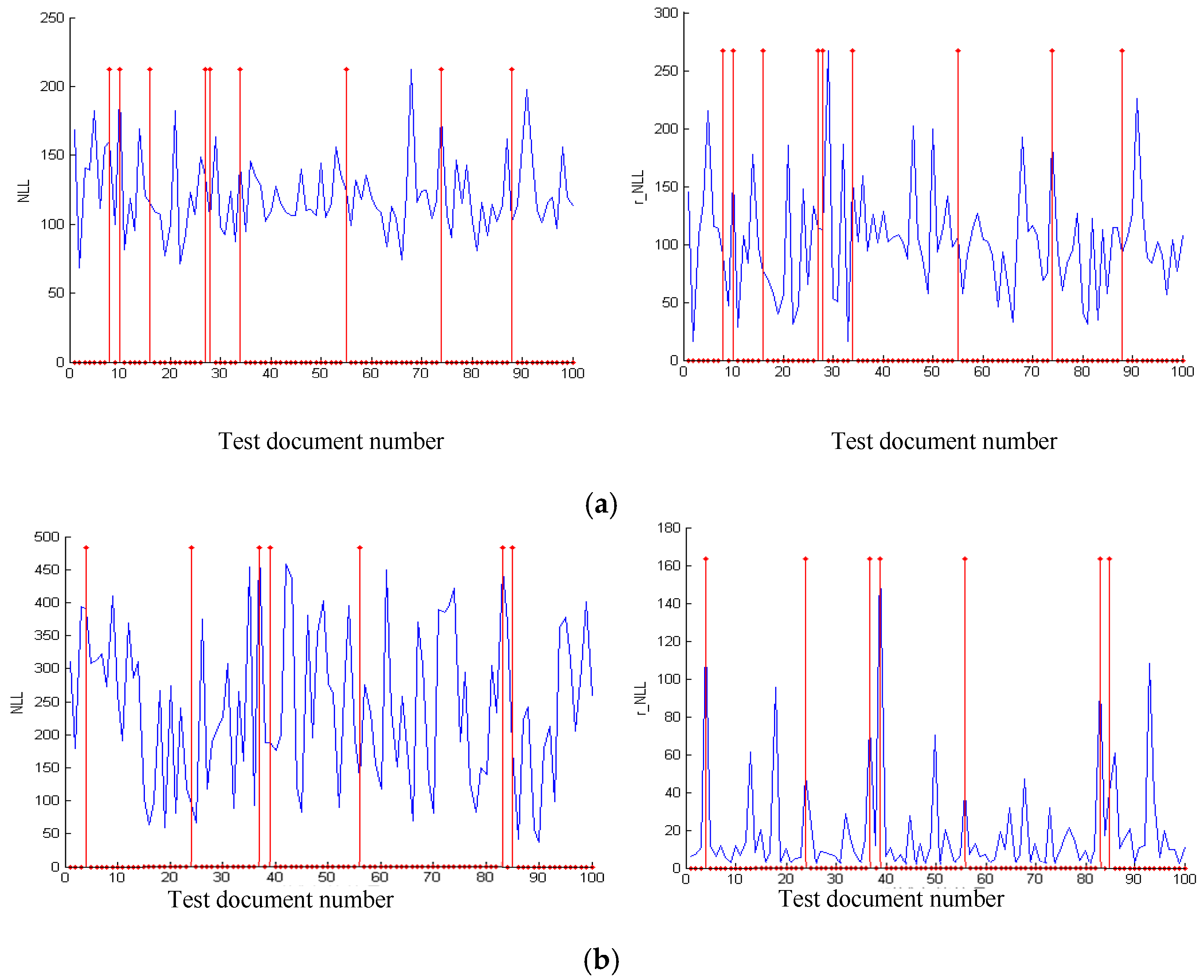
In the text mining and statistic inference of nature language, perplexity is always used to evaluate the performance of model, which is computed by $perp\left(X^{\mathrm{test}}|\widehat{\mathsf{\phi }}\right)=\exp \left\{-\log p\left(X^{\mathrm{test}}|\widehat{\mathsf{\phi }}\right)/N^{\mathrm{test}}\right\}$. $\widehat{\mathsf{\phi }}$ denotes the parametric estimation of trained model, $X^{\mathrm{test}}$ and $N^{\mathrm{test}}$ are test dataset and observed samples respectively. Perplexity is the negative log likelihood (NLL) $-\log p\left(X^{\mathrm{test}}|\widehat{\mathsf{\phi }}\right)$ divided by the number of observed samples $N^{\mathrm{test}}$. As described in above, the computation of perplexity is mainly the NLL computation of trained model, and NLL denotes the cross entropy of trained model and unknown testing data. Perplexity represents the uncertainty of trained model for unknown test set’s estimation. Therefore, the lower the NLL value is, the better the model performance is.

In our RTM, NLL can be computed for motion topic and region of test video clip. The parameters estimation of trained model and a test video clip are learning in RTM, the learned local motion topic weight estimation $\hspace{0.17em}{\tilde{\pi }}_t$ and global parameter estimation ${\tilde{\varsigma }}_{ir}$, ${\tilde{\theta }}_{\omega rt}$ of original trained model is computed for NLL of test clips.

$$\begin{array}{ll}\mathrm{rLDA}\_\mathrm{NLL}\left(X^{\mathrm{test}}|{\tilde{\pi }}_t,{\tilde{\varsigma }}_{ir},{\tilde{\theta }}_{\omega rt}\right)& =-{\displaystyle {\sum }_{n=1}^{N^{\mathrm{test}}}}\log \left({\displaystyle {\sum }_{r=1}^R}{\tilde{\varsigma }}_{ir}{\displaystyle {\sum }_{t=1}^T}\hspace{0.17em}{\tilde{\pi }}_t{\tilde{\theta }}_{x_n^{\mathrm{test}}=\omega ,rt}\right)\\ & =-N_{(\omega ,i)}\log \left({\displaystyle {\sum }_{r=1}^R}{\tilde{\varsigma }}_{ir}{\displaystyle {\sum }_{t=1}^T}\hspace{0.17em}{\tilde{\pi }}_t{\tilde{\theta }}_{\omega rt}\right)\end{array}$$

(24)

Besides, t_NLL and r_NLL are computed by:

$$\begin{array}{ll}\mathrm{t}\_\mathrm{NLL}\left(X^{\mathrm{test}}|{\tilde{\varsigma }}_{ir},{\tilde{\theta }}_{\omega rt}\right)& =-{\displaystyle {\sum }_{n=1}^{N^{\mathrm{test}}}}\log \left(\mathbb{I}\left(t_n=t\right){\displaystyle {\sum }_{r=1}^R}{\tilde{\varsigma }}_{ir}{\tilde{\theta }}_{x_n^{\mathrm{test}}=\omega ,rt}\right)\\ & =-N_{(\omega ,i,t)}\log \left({\displaystyle {\sum }_{r=1}^R}{\tilde{\varsigma }}_{ir}{\tilde{\theta }}_{\omega rt}\right)\end{array}$$

(25)

$$\begin{array}{ll}\mathrm{r}\_\mathrm{NLL}\left(X^{\mathrm{test}}|{\tilde{\pi }}_t,{\tilde{\theta }}_{\omega rt}\right)& =-{\displaystyle {\sum }_{n=1}^{N^{\mathrm{test}}}}\log \left(\mathbb{I}\left(r_n=r\right){\displaystyle {\sum }_{t=1}^T}\hspace{0.17em}{\tilde{\pi }}_t{\tilde{\theta }}_{x_n^{\mathrm{test}}=\omega ,rt}\right)\\ & =-N_{(\omega ,r)}\log \left({\displaystyle {\sum }_{t=1}^T}\hspace{0.17em}{\tilde{\pi }}_t{\tilde{\theta }}_{\omega rt}\right)\end{array}$$

(26)

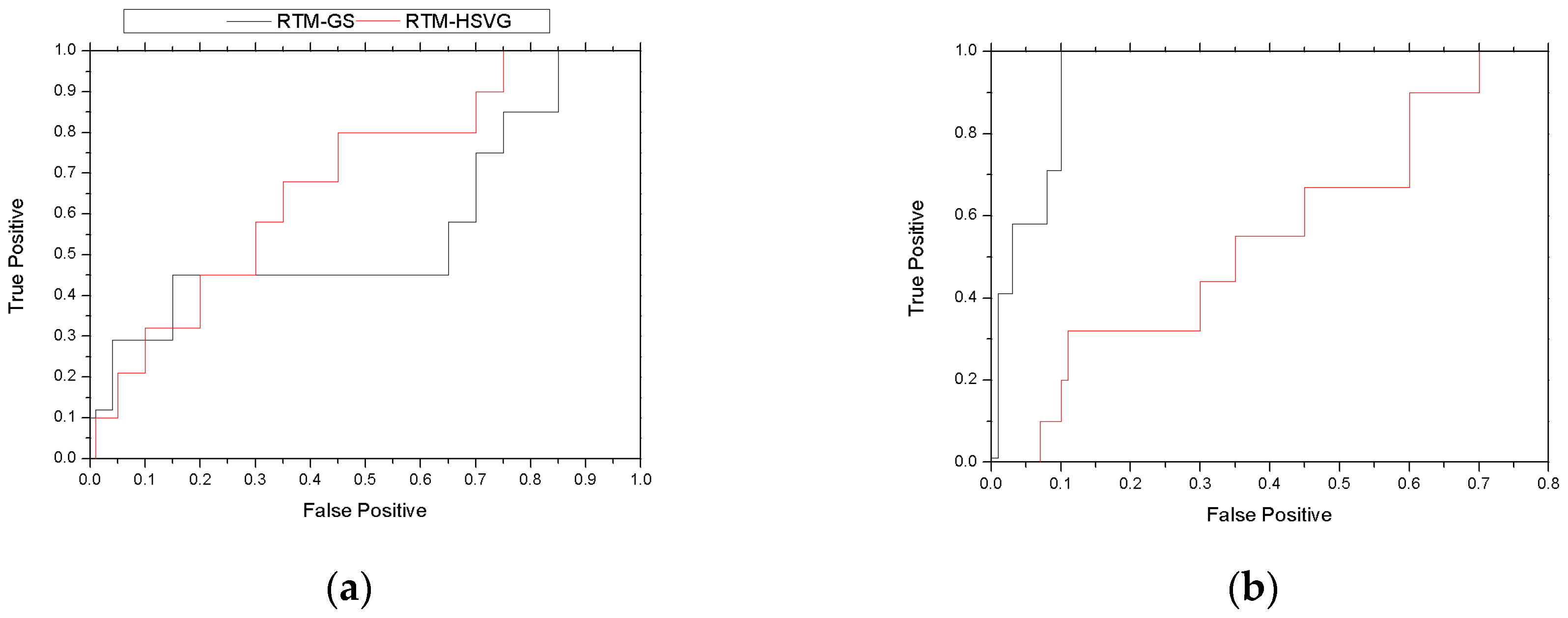
t_NLL is used to evaluate the performance of learning motion topic by our model, and r_NLL is used to evaluate the performance of learning motion region. Meanwhile, because of the samples number difference between different regions, the abnormal events probabilities of the region including few samples is lower, so we add a sample number weight for each region. We regard the five most regions of r_NLL value as the most possible abnormal events regions. Furthermore, we utilize receiver operating characteristic curve (ROC) and AUC (area under ROC) to evaluate the abnormal detecting performance of our model, which are independent of threshold selection. Obviously, for ROC, the closer to the top left corner, the performance of abnormal detection is better. Similarly, the closer to 1 the AUC value is, the better the performance of abnormal detection. The running platform of experiment is shown in

Table 1. Software and hardware platform.

CPU	Intel® Core(TM) 2 Duo CPU E8400 @ 3.00 GHz 3.00 GHz
Memory	2.00 G
OS	Window7
Programing platform	Python 2.7.5

.

4.2. Datasets and Parameter Settings

In order to get the comprehensive evaluation of our model and its inference algorithm, we analyze the performance based on two types of dataset. The first one is a simulation video dataset constructed by specific steps, and the second one is a real video dataset.

4.2.1. Simulation Video Dataset

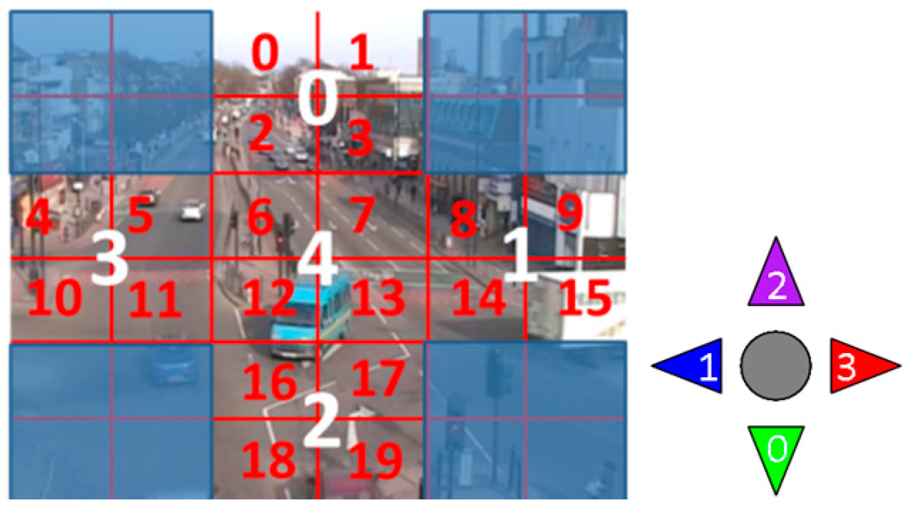
We make a simulation video dataset for simulating the traffic intersection. Each image of a frame was divided into a 6 by 6 grid (a total of 36 positions) and five valid regions (including the sides of up, middle, down, right, and left). Meanwhile, each valid region is composed by 4 grids, that there are in total of 4 × 5 = 20 locations to simulate one center and four directions of traffic intersection, as shown in Figure 3.

In Figure 3, white texts represent the valid region number $r\in \left\{0,1,2,3,4\right\}$, and red texts represent the valid location number $i\in \left\{0,\dots ,19\right\}$. Four directions are represented as down (green), left (blue), up (purple) and right (red), whose number is $\omega \in \left\{0,1,2,3\right\}$. Then, the number of locations is $I=20$, and the number of motion directions is $\mathsf{\Omega }=4$. $\left(i,\omega \right)$ is used to denote a motion word, where $i\in \left\{0,\dots ,I-1\right\}$,$\omega \in \left\{0,\dots ,\mathsf{\Omega }-1\right\}$, and the number of motion words is $W=I\times \mathsf{\Omega }=80$. The latent motion topic is constructed by combining region number $r$ and direction number $\omega$. Regarding $\left(i\in r=0,\omega =0\right)$ as an instance, it means that one location of region 0(that location number is one of $\left\{0,1,2,3\right\}$) is moving in direction 0(down). Then, normal and abnormal motions are able to be constructed by above way. There are five kinds of normal motion states and two kinds of abnormal motion states. The generative algorithm of simulation video is described below:

Generate an initial motion direction $\omega$ randomly.

Choose a motion topic, where the probability of abnormal motion topic is 5%, and the probability of abnormal motion topic is 95%.

Generate 100 samples by

Based on the chosen motion topic, choose a motion state randomly.

Based on the chosen motion state, generate an observed sample $\left({\omega }^{\prime },\hspace{0.17em}\hspace{0.17em}{i}^{\prime }\right)$ randomly.

Figure 4 shows the generated training set and test set by above steps. The color of arrow represents the direction, and the brightness represents the probability in motion topic.

4.2.2. Real Video Dataset

We use the QMUL street intersection dataset [41] for evaluating abnormality detection performance of this model. This standard video is 50 min in length, frame rates are 30 fps, resolution is 360 × 288, and there are 90,000 frames. Video codec is mpeg-4 compression encoding. The whole traffic light cycle is about 1.5 min; the average duration of abnormal event is 4.3 s (129 frames).

In our experiment, we divide whole video into 250 clips; each clip is 12 s (360 frames). The top 14.36 min (30 documents) is training dataset, and the last 10 min (50 documents) is test dataset. Each scene of a clip is first divided into a 4 by 4 grid (a total of 16 positions) and five valid regions. After cutting off the part of sky and generating motion code book for model training, RTM-HSVG (RTM is learned and inference by Hybrid Stochastic Variational Gibbs Sampling) and RTM-GS (RTM is learned and inference by Gibbs Sampling) then computes the negative loglikelihood of every region as a score in each test clip and abnormality clips are picked up while its abnormality score exceed 1.5 times of average. The parameter settings are shown in

Table 2. Parameter settings of RTM-HSVG and RTM-GS.

RTM-GS	RTM-HSVG
Burn-in time $N=2000$; After Markov chain convergence, sampling at intervals of 100 times; the total number of sampling is $S=20$; $T=18$; $R=20$; The hyper parameter is $\alpha =0.3$; $\beta =1.2$; $\lambda =0.3$	Burn-in time $N=400$; After Markov chain convergence, sampling at intervals of 10 times; the total number of sampling is $S=10$; $T=36$;$R=20$; The hyper parameter is $\alpha =0.3$; $\beta =1.2$; $\lambda =0.3$

4.3. Experimental Results

4.3.1. Simulation Experiment of Visualization Traffic Intersection

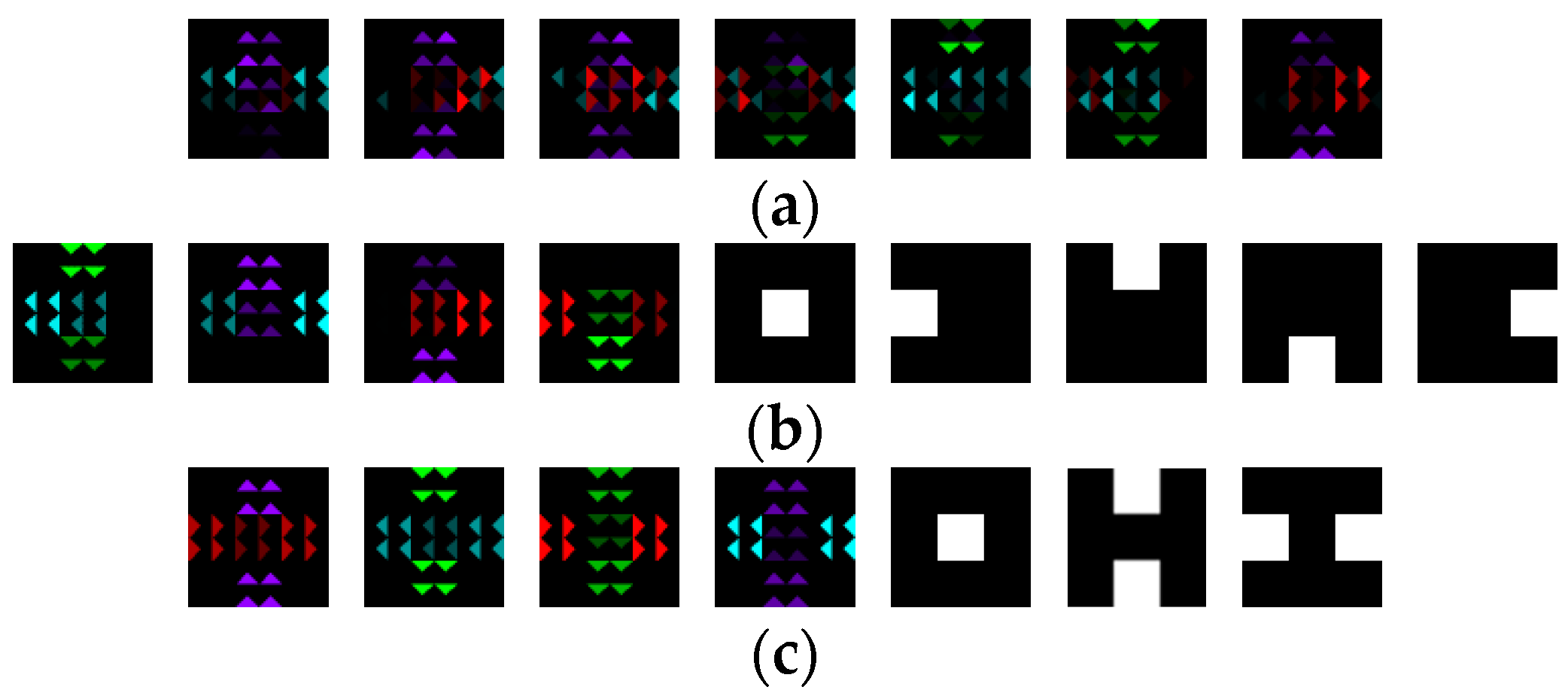
Firstly, the motion topics and regions discovered by RTM-GS and RTM-HSVG is shown in Figure 5, where Figure 5a shows the seven random simulated abnormal motions. The number of simulated training documents is same as the number of test set, which is 100.

As can be seen from Figure 5, although RTM-GS discovers more latent regions, a refined topic division is obtained by RTM-HSVG. Furthermore, in RTM-HSVG, the two roads with same direction are combined to a latent region, which is capable of moving crossroad. It is more reasonable that motions comply with traffic rules of a same road are the same.

To compare the abilities of our model to discover abnormal motion, the NLL and r_NLL comparisons of our model and actual values is shown in Figure 6.

As shown in Figure 6, for r_NLL curve, the accuracy of RTM-GS seems to be higher than RTM-HSVG. Nonetheless, for NLL curve, RTM-HSVG obtained a higher accuracy. As HSVG is a kind of stochastic algorithm, it cause a volatile shocks in r_NLL curve. It also suggests that our stochastic online algorithm need to introduce more motion region information to acid early-warning. The difference between RTM-GS and RTM-HSVG is also able to be observed in their ROC and AUC, which is shown in Figure 7.

As shown in Figure 7, the area under NLL ROC of RTM-HSVG is 0.68, and RTM-GS is 0.56. This result again explains that the comprehensive accuracy of RTM-HSVG is better than RTM-GS. On the other hand, the area under r_NLL ROC of RTM-HSVG is 0.64, and RTM-GS is 0.97, which illustrates that the performance of learning motion region of RTM-GS is better than RTM-HSVG. These simulated experimental results show the validity of RTM for discovering motion topic and motion region.

4.3.2. Real Video Experiment

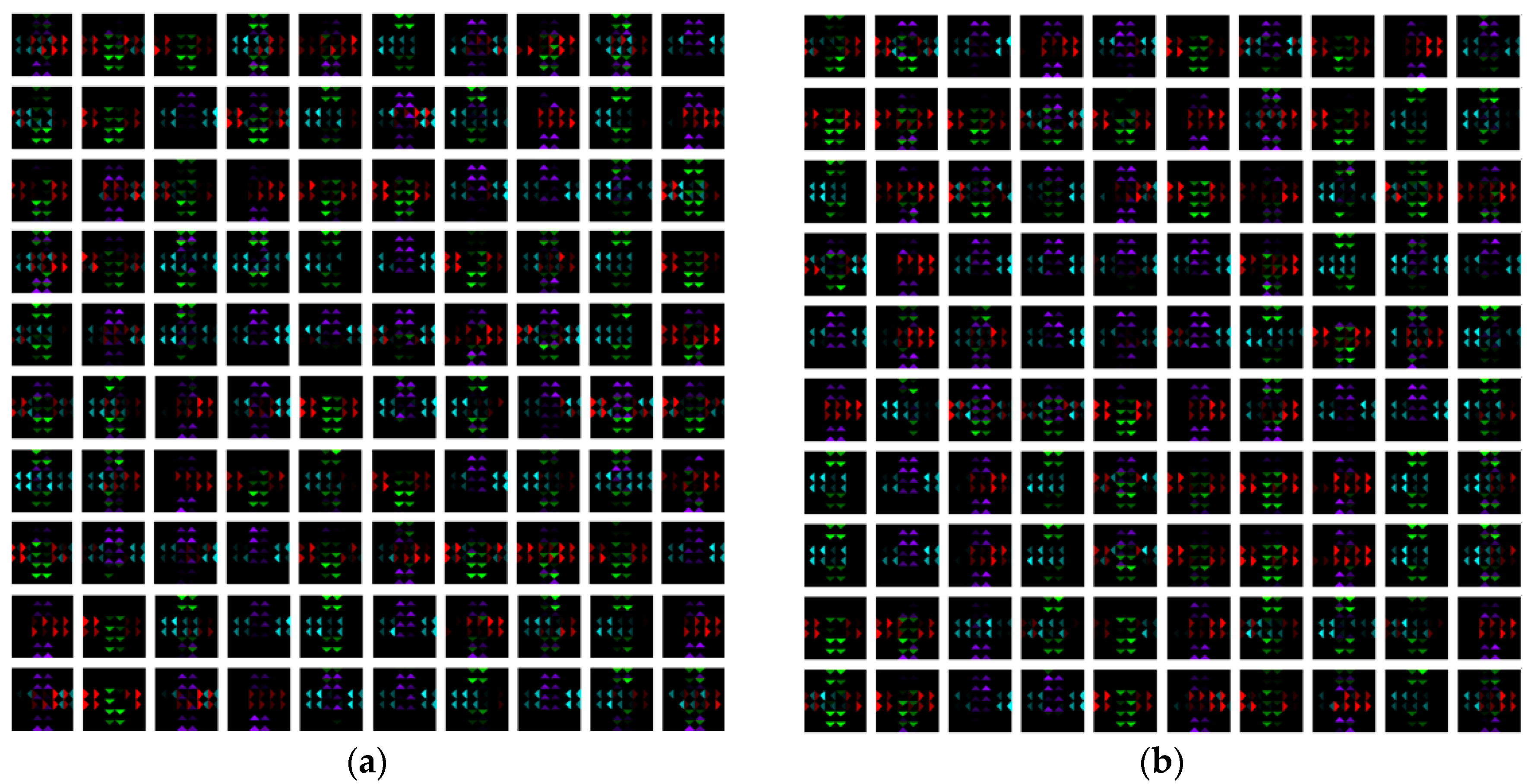
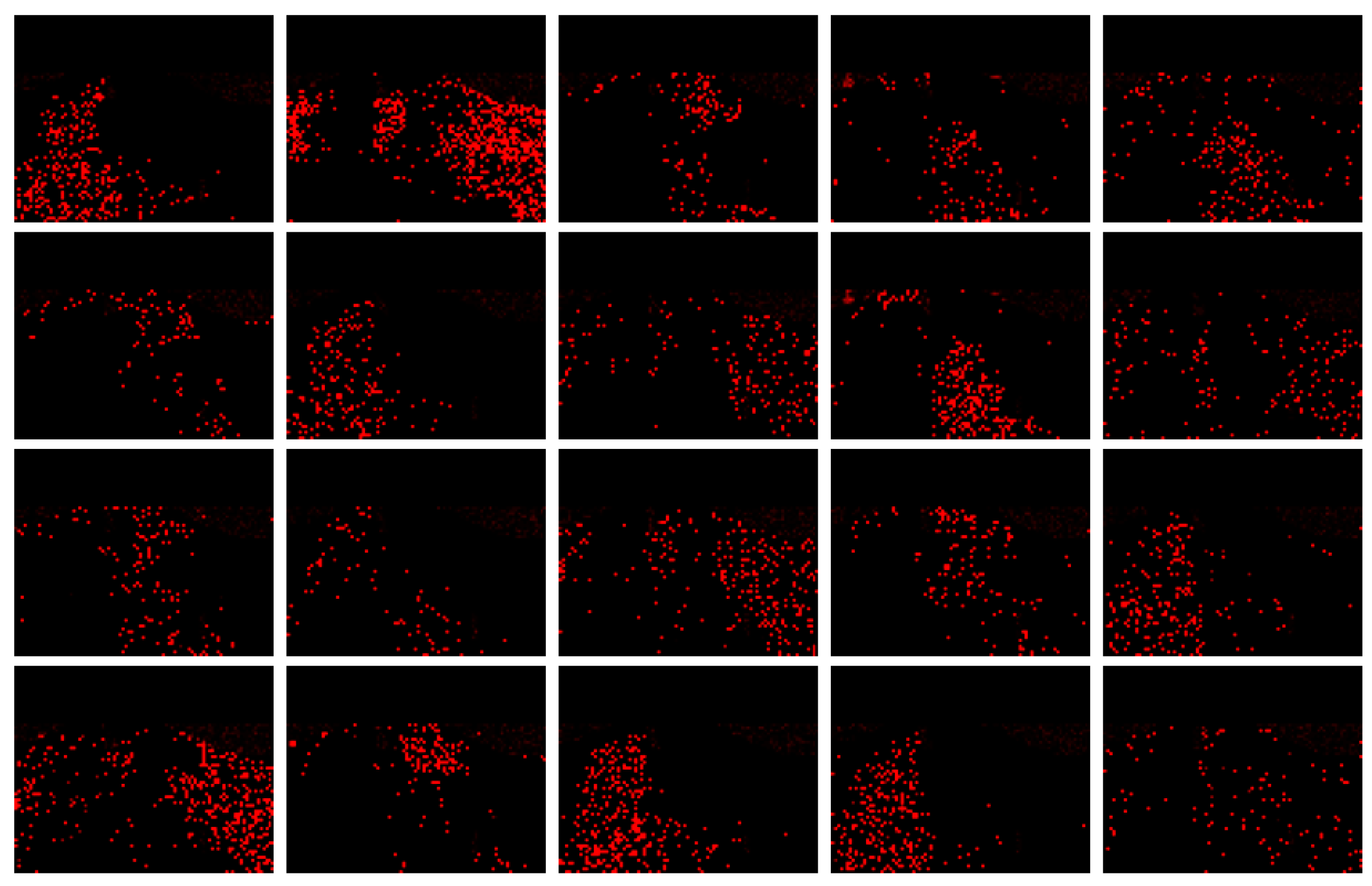
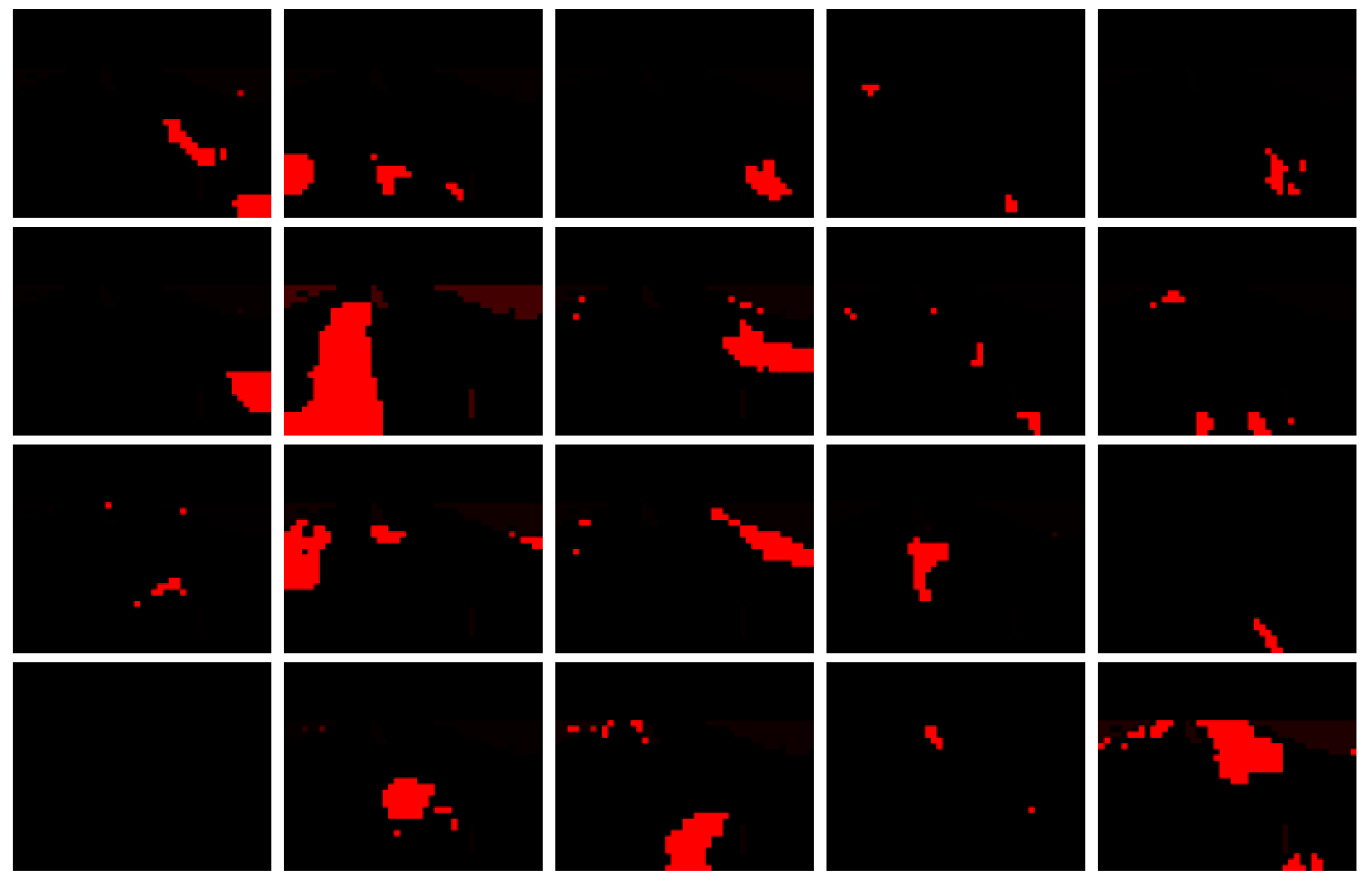
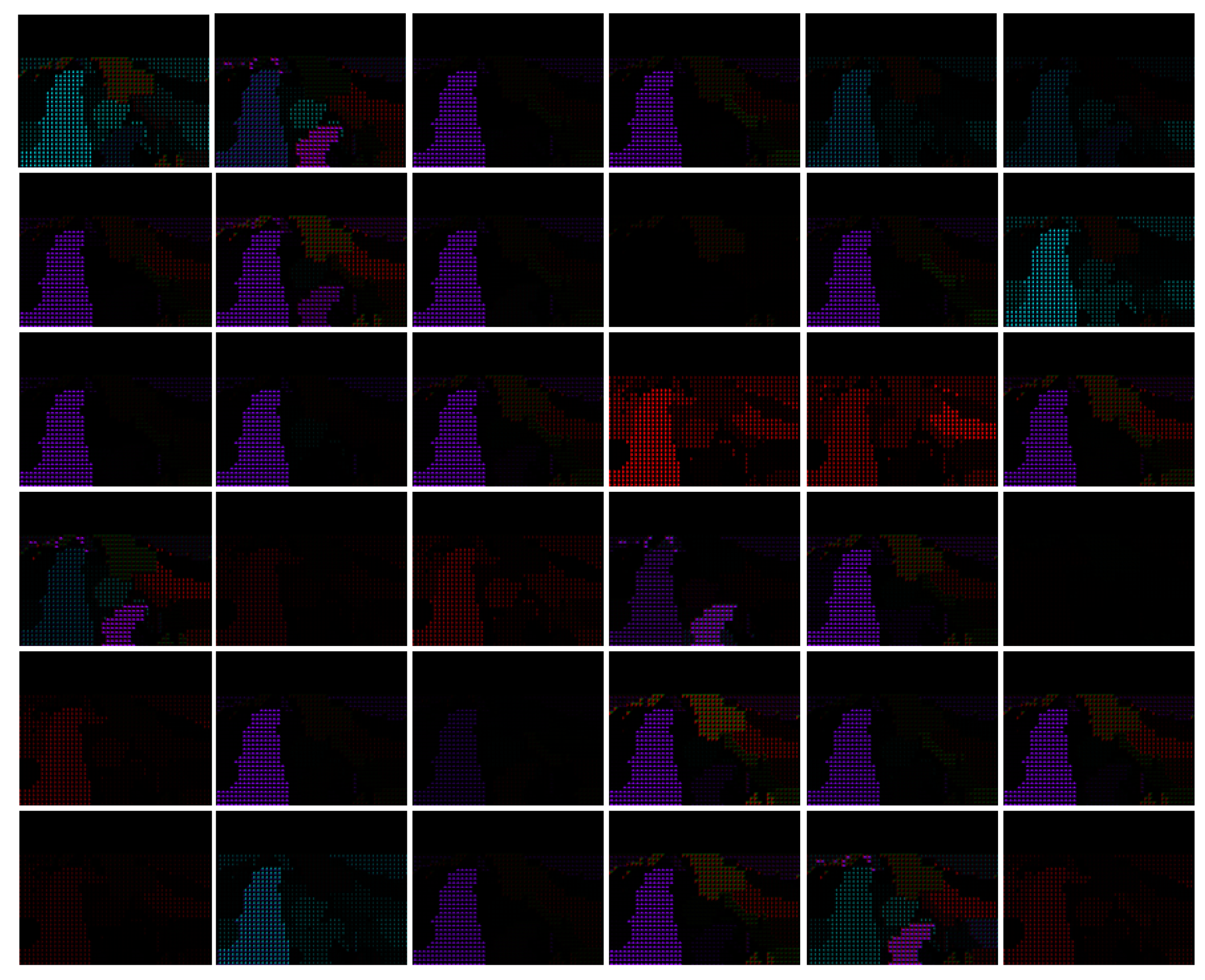
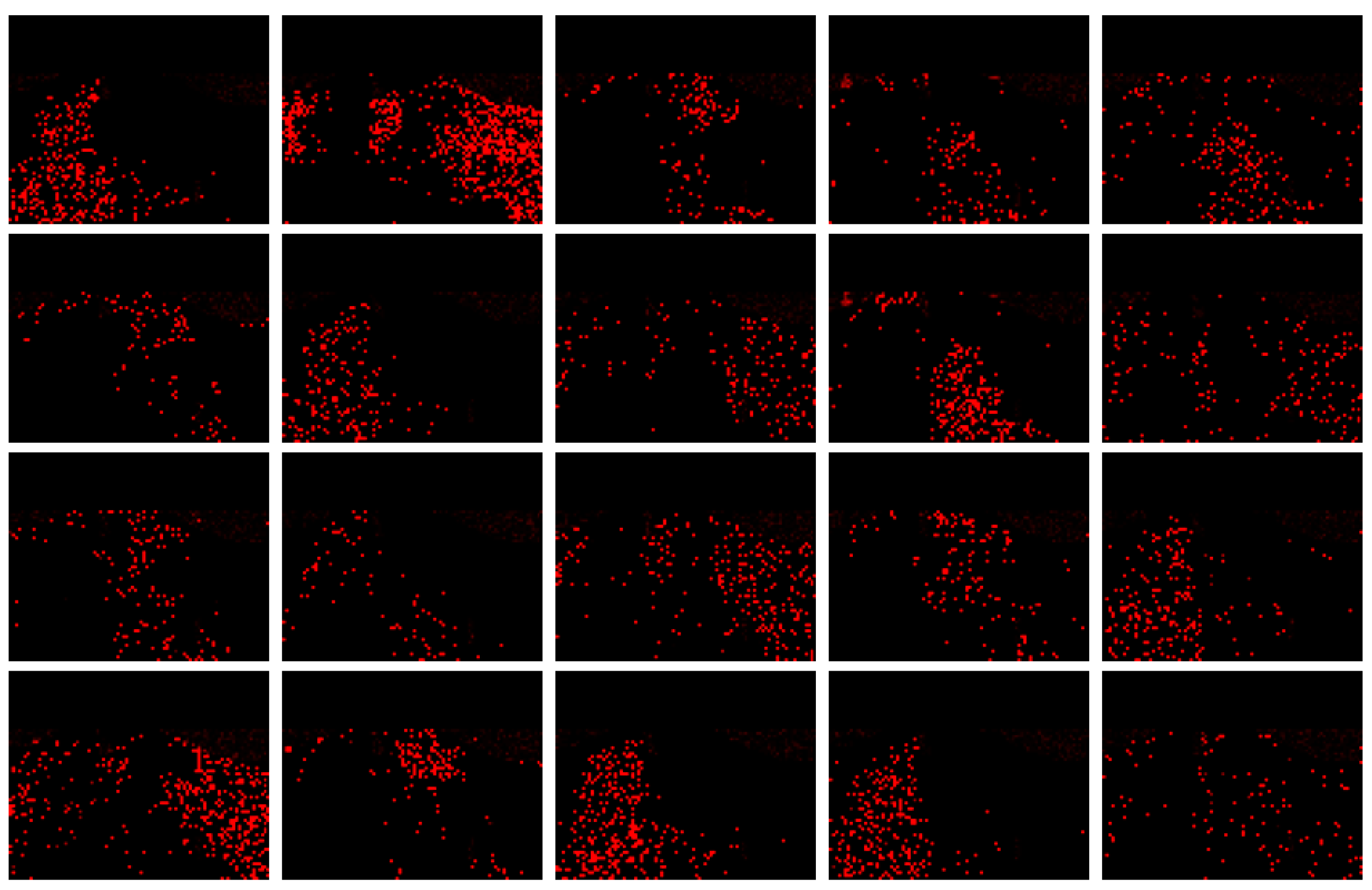
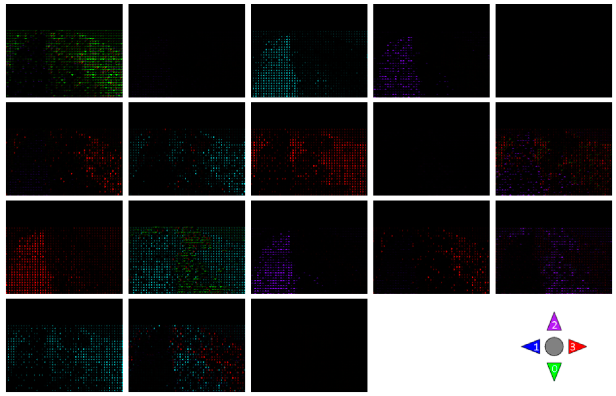
Likewise, for QUML dataset, the motion topics and regions discovered by RTM-GS and RTM-HSVG is shown in Figure 8, Figure 9, Figure 10 and Figure 11 respectively.

According to the comparisons of latent motion topic and motion regions discovered in above figures, RTM-GS obtained more clearly atomic motion patterns, which form the motion topic. Nevertheless, RTM-HSVG obtained a more focused clustering in both motion topic and region, and the direction representation of RTM-HSVG is richer (observed from the mixture of four directions). This is because the Markov chain state space of large-scale dataset is larger; it needs a longer burn-in time for Markov chain convergence. Even if RTM-HSVG has a shorter burn-in time, it also obtained a better performance than RTM-GS.

In order to test the impact of burn-in time on performance of our model, the burn-in time of RTM-GS is increasing to four times, and the iteration-times is set as 8000. Then, the motion topics and regions results are shown in Figure 12 and Figure 13.

In comparison with Figure 8 and Figure 12 as well as Figure 9 and Figure 13, we find that longer burn-in time makes a more focused clustering in both motion topic and region. Nevertheless, it is difficult to decide when Markov chain is convergent in Gibbs sampling, and longer burn-time is at the expense of time efficiency. Therefore, RTM-HSVG is more efficient than RTM-GS as an online algorithm. Meanwhile, we find that a larger number of topics can make more clear motion topics, which also makes more repeated latent topics. Therefore, it illustrates that the number of topics and regions are important aspects to decide performance of RTM.

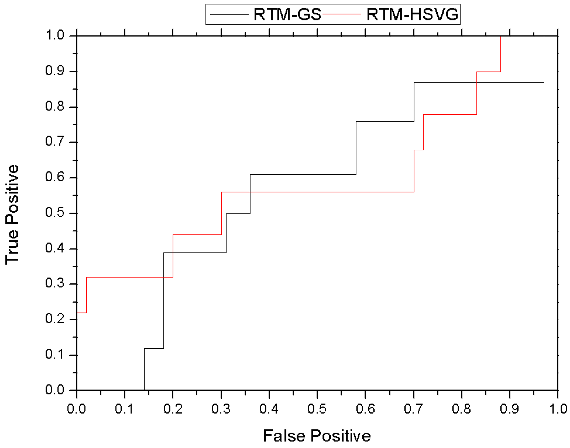
The ROC curve comparison of RTM-HSVG and RTM-GS is shown in the Figure 14. As shown in Figure 14, the area under ROC of RTM-HSVG is 0.59, and RTM-GS is 0.577. These results again indicate that RTM-HSVG can improve the accuracy of abnormal event detection in comparison with RTM-GS.

At last, several abnormal events discovered by RTM-HSVG are shown in Figure 15, and the regions of abnormal motion are labeled by dark red.

Figure 15a shows an abnormal event in 33rd clips (37,410~37,769), its motion region is number 6, and NLL = 724,951.87. A fire vehicle is driving into the crossing from right and interrupting the vertical traffic.

Figure 15b shows an abnormal event in 25th clips (34,538~34,897), its motion region is number 9, and NLL = 753,774.17. A car is turning right illegally.

Figure 15c shows an abnormal event in 15th clips (30,948~31,307), its motion region is number 13, and NLL = 792,248.81. A car makes a U-turn illegally.

Figure 15d shows an abnormal event in 14th clips (30,589~30,948), its motion region is number 15, and NLL = 819,426.78. A fire vehicle is driving into the crossing from lift and interrupting the vertical traffic.

From the above experimental results, we can see that RTM is able to discover motion topics and motion regions efficiently. Specially, the HSVG inference algorithm designed for RTM is better than Gibbs sampling on accuracy and time efficiency. Therefore, we can anticipate that RTM-HSVG is a potential method for real-time video mining.

5. Conclusions

To solve the problem that traditional topic model is unable to process video in real-time and model motion regional information, we proposed a RTM and designed its hybrid stochastic variational Gibbs sampling algorithm. In RTM, observation data not only has the motion topic label but also has region label of its position. In our HSVG algorithm, the local weight ${\mathsf{\pi }}_j$ is collapsed locally for retaining the high relativities between local latent variable set and local weight at first, and then local Gibbs sampling is introduced for retaining low relativities of local latent variable set $T_j$. For global variational parameters ${\varsigma }_{ir}$, ${\nu }_r$, and ${\mu }_{\omega rt}$, the stochastic natural gradient methods are adopted, which make RTM capable of processing massive video dataset in real time. The experimental results on simulate and real dataset show that the proposed RTM-HSVG improves the anomaly detection performance in comparison to the RTM-GS.

References

- Dai, K.; Zhang, J.; Li, G. Video mining: Concepts, approaches and applications. In Proceedings of the IEEE 12th International Multi-Media Modelling Conference Proceedings, Beijing, China, 4–6 January 2006. [Google Scholar]
- Chen, S.C.; Shyu, M.L.; Zhang, C.; Strickrott, J. A multimedia data mining framework: Mining information from traffic video sequences. Intell. Inf. Syst. 2002, 19, 61–77. [Google Scholar] [CrossRef]
- Blei, D.; Carin, L.; Dunson, D. Probabilistic topic models. IEEE Signal Process. Mag. 2010, 27, 55–65. [Google Scholar] [CrossRef] [PubMed]
- Wang, L.H.; Zhao, G.G.; Sun, D.H. Modeling documents with event model. Algorithms 2015, 8, 562–572. [Google Scholar] [CrossRef]
- Blei, D.M.; Ng, A.Y.; Jordan, M.I. Latent dirichlet allocation. Mach. Learn. Res. 2003, 3, 993–1022. [Google Scholar]
- Griffiths, T.L.; Steyvers, M. Finding scientific topics. Proc. Natl. Acad. Sci. USA 2004, 101, 5228–5235. [Google Scholar] [CrossRef] [PubMed] [Green Version]
- Teh, Y.W.; Jordan, M.I.; Beal, M.J.; Blei, D.M. Hierarchical dirichlet processes. Am. Stat. Assoc. 2006, 101, 1566–1581. [Google Scholar] [CrossRef]
- Larlus, D.; Verbeek, J. Category Level Object Segmentation by Combining Bag-of-Words Models with Dirichlet Processes and Random Fields. Int. J. Comput. Vis. 2010, 88, 238–253. [Google Scholar] [CrossRef]
- Hofmann, T. Probabilistic latent semantic analysis. In Proceedings of the Fifteenth Conference on Uncertainty in Artificial Intelligence, Stockholm, Sweden, 30 July–1 August 1999; pp. 289–296. [Google Scholar]
- Wang, X.; Ma, X.; Grimson, W.E.L. Unsupervised Activity Perception in Crowded and Complicated Scenes Using Hierarchical Bayesian Models. IEEE Trans. Pattern Anal. 2009, 31, 539–555. [Google Scholar] [CrossRef] [PubMed] [Green Version]
- Wang, X.; Ma, K.T.; Ng, G.W. Trajectory analysis and semantic region modeling using a nonparametric Bayesian model. In Proceedings of the IEEE Conference on Computer Vision and Pattern Recognition, Anchorage, AK, USA, 23–28 June 2008; pp. 1–8. [Google Scholar]
- Li, J.; Gong, S.; Xiang, T. Scene segmentation for behaviour correlation. In Proceedings of the European Conference on Computer Vision, Marseille, France, 12–18 October 2008; pp. 383–395. [Google Scholar]
- Li, J. Learning behavioural context. Int. J. Comput. Vis. 2012, 97, 276–304. [Google Scholar] [CrossRef]
- Hospedales, T.M.; Li, J.; Gong, S.; Xiang, T. Identifying rare and subtle behaviors: A weakly supervised joint topic model. Int. J. Comput. Vis. 2012, 33, 2451–2464. [Google Scholar] [CrossRef] [PubMed] [Green Version]
- Emonet, R.; Varadarajan, J.; Odobez, J. Extracting and locating temporal motifs in video scenes using a hierarchical non parametric Bayesian model. Int. J. Comput. Vis. 2011, 32, 3233–3240. [Google Scholar]
- Fu, W.; Wang, J.; Lu, H.; Ma, S. Dynamic scene understanding by improved sparse topical coding. Pattern Recogn. 2013, 46, 1841–1850. [Google Scholar] [CrossRef]
- Yuan, J.; Zheng, Y.; Xie, X. Discovering regions of different functions in a city using human mobility and POIs. In Proceedings of the 18th ACM SIGKDD International Conference on Knowledge Discovery and Data Mining, Beijing, China, 12–16 August 2012; pp. 186–194. [Google Scholar]
- Farrahi, K.; Gatica-Perez, D. Discovering routines from large-scale human locations using probabilistic topic models. ACM Trans. Intell. Syst. Technol. 2011, 2. [Google Scholar] [CrossRef]
- Zhao, Z.; Xu, W.; Chen, D. EM-LDA model of user behavior detection for energy efficiency. In Proceedings of the IEEE International Conference on System Science and Engineering, Shanghai, China, 11–13 July 2014; pp. 295–300. [Google Scholar]
- Yu, R.; He, X.; Liu, Y. GLAD: Group anomaly detection in social media analysis. In Proceedings of the 20th ACM SIGKDD International Conference on Knowledge Discovery and Data Mining, New York, NY, USA, 24–27 August 2014; pp. 372–381. [Google Scholar]
- Kinoshita, A.; Takasu, A.; Adachi, J. Real-time traffic incident detection using a probabilistic topic model. J. Intell. Inf. Syst. 2015, 54, 169–188. [Google Scholar] [CrossRef]
- Hospedales, T. Video behaviour mining using a dynamic topic model. Int. J. Comput. Vis. 2012, 98, 303–323. [Google Scholar] [CrossRef]
- Fan, Y.; Zhou, Q.; Yue, W.; Zhu, W. A dynamic causal topic model for mining activities from complex videos. Multimed. Tools Appl. 2017, 10, 1–16. [Google Scholar] [CrossRef]
- Hu, X.; Hu, S.; Zhang, X.; Zhang, H.; Luo, L. Anomaly detection based on local nearest neighbor distance descriptor in crowded scenes. Sci. World J. 2014, 2014, 632575. [Google Scholar] [CrossRef] [PubMed]
- Pathak, D.; Sharang, A.; Mukerjee, A. Anomaly localization in topic-based analysis of surveillance videos. In Proceedings of the IEEE Winter Conference on Applications of Computer Vision, Waikoloa, HI, USA, 5–9 January 2015; pp. 389–395. [Google Scholar]
- Jeong, H.; Yoo, Y.; Yi, K.M.; Choi, J.Y. Two-stage online inference model for traffic pattern analysis and anomaly detection. Mach. Vis. Appl. 2014, 25, 1501–1517. [Google Scholar] [CrossRef]
- Kaviani, R.; Ahmadi, P.; Gholampour, I. Incorporating fully sparse topic models for abnormality detection in traffic videos. In Proceedings of the International Conference on Computer and Knowledge Engineering, Mashhad, Iran, 29–30 October 2014; pp. 586–591. [Google Scholar]
- Isupova, O.; Kuzin, D.; Mihaylova, L. Anomaly detection in video with Bayesian nonparametrics. arXiv, 2016arXiv:1606.08455v1.
- Zou, J.; Chen, X.; Wei, P.; Han, Z.; Jiao, J. A belief based correlated topic model for semantic region analysis in far-field video surveillance systems. In Proceedings of the Pacific-Rim Conference on Multimedia, Nanjing, China, 13–16 December 2013; pp. 779–790. [Google Scholar]
- Haines, T.S.F.; Xiang, T. Video topic modelling with behavioural segmentation. In Proceedings of the ACM International Workshop on Multimodal Pervasive Video Analysis, Firenze, Italy, 29 October 2010; pp. 53–58. [Google Scholar]
- Gasparini, M. Markov chain monte carlo in practice. Technometrics 1997, 39, 338. [Google Scholar] [CrossRef]
- Schölkopf, B.; Platt, J.; Hofmann, T. A collapsed variational bayesian inference algorithm for latent dirichlet allocation. Adv. Neural Inf. Process. Syst. 2007, 19, 1353–1360. [Google Scholar]
- Hoffman, M.D.; Blei, D.M.; Bach, F. Online learning for latent dirichlet allocation. In Proceedings of the International Conference on Neural Information Processing Systems, Vancouver, BC, Canada, 6–9 December 2010; pp. 856–864. [Google Scholar]
- Mimno, D.; Hoffman, M.; Blei, D. Sparse stochastic inference for latent dirichlet allocation. arXiv, 2012arXiv:1206.6425.
- Girolami, M.; Calderhead, B. Riemann manifold langevin and hamiltonian monte carlo methods. J. R. Stat. Soc. 2015, 73, 123–214. [Google Scholar] [CrossRef]
- Welling, M.; Teh, Y.W. Bayesian learning via stochastic gradient langevin dynamics. In Proceedings of the International Conference on Machine Learning, Bellevue, WA, USA, 28 June–2 July 2011; pp. 681–688. [Google Scholar]
- Patterson, S.; Teh, Y.W. Stochastic gradient riemannian langevin dynamics on the probability simplex. In Advances in Neural Information Processing Systems, Harrahs and Harveys, Lake Tahoe, 5–10 December 2013. 3102–3110.
- Isupova, O.; Kuzin, D.; Mihaylova, L. Learning methods for dynamic topic modeling in automated behavior analysis. IEEE Trans. Neural Netw. Learn. 2017, 99, 1–14. [Google Scholar] [CrossRef] [PubMed]
- Rosen-Zvi, M.; Chemudugunta, C.; Griffiths, T.; Smyth, P.; Steyvers, M. Learning author-topic models from text corpora. ACM Trans. Inf. Syst. 2010, 28, 1–38. [Google Scholar] [CrossRef] [Green Version]
- Bao, S.; Xu, S.; Zhang, L.; Yan, R.; Su, Z.; Han, D.; Yu, Y. Mining social emotions from affective text. IEEE Trans. Knowl. Data Eng. 2012, 24, 1658–1670. [Google Scholar] [CrossRef]
- Junction Dataset. Available online: http://www.eecs.qmul.ac.uk/~sgg/QMUL_Junction_Datasets/Junction/Junction.html (accessed on 29 May 2017).
Figure 1.
Diagram of video topic modeling.
Figure 2.
Graphical model of RTM.
Figure 3.
Directions and regions of simulation video
Figure 4.
Generated simulation datasets. (a) Training set. (b) Test set.
Figure 5.
Motion topics and regions discovered by RTM-GS and RTM-HSVG in simulation dataset (a) The seven random simulate abnormal motions. (b) The four motion topics and five regions discovered by RTM-GS. (c) The four motion topics and three regions discovered by RTM-HSVG.
Figure 6.
The NLL and r_NLL comparisons of our model and actual values. (a) NLL (left and blue) and r_NLL (right and blue) comparisons of RTM-HSVG. (b) NLL (left and blue) and r_NLL (right and blue) comparisons of RTM-GS.
Figure 7.
Comparative results of ROC. (a) Comparative results on NLL. (b) Comparative results on r_NLL.
Figure 8.
Twenty latent motion regions discovered by RTM-GS.
Figure 9.
Eighteen latent motion topics discovered by RTM-GS.
Figure 10.
Twenty latent motion regions discovered by RTM-HSVG.
Figure 11.
Thirty-six latent motion topics discovered by RTM-HSVG.
Figure 12.
Twenty latent motion regions discovered by RTM-GS on longer burn-in time.
Figure 13.
Eighteen latent motion topics discovered by RTM-GS on longer burn-in time.
Figure 14.
Comparative results of ROC on real video.
Figure 15.
Locating abnormal events by RTM-HSVG.