Long Length Document Classification by Local Convolutional Feature Aggregation

1
School of Electronic and Information Engineering, Nanjing University of Information Science and Technology, Nanjing 210044, China
2
State Grid Corporation of China, Beijing 100031, China
3
NARI Group Corporation of China/State Grid Electric Power Research Institute, Nanjing 211106, China
*
Author to whom correspondence should be addressed.
Algorithms 2018, 11(8), 109; https://doi.org/10.3390/a11080109
Submission received: 7 June 2018
/
Revised: 17 July 2018
/
Accepted: 20 July 2018
/
Published: 24 July 2018
Abstract
:The exponential increase in online reviews and recommendations makes document classification and sentiment analysis a hot topic in academic and industrial research. Traditional deep learning based document classification methods require the use of full textual information to extract features. In this paper, in order to tackle long document, we proposed three methods that use local convolutional feature aggregation to implement document classification. The first proposed method randomly draws blocks of continuous words in the full document. Each block is then fed into the convolution neural network to extract features and then are concatenated together to output the classification probability through a classifier. The second model improves the first by capturing the contextual order information of the sampled blocks with a recurrent neural network. The third model is inspired by the recurrent attention model (RAM), in which a reinforcement learning module is introduced to act as a controller for selecting the next block position based on the recurrent state. Experiments on our collected four-class arXiv paper dataset show that the three proposed models all perform well, and the RAM model achieves the best test accuracy with the least information.
1. Introduction
Document classification is a classic problem in the field of natural language processing (NLP). Its purpose is to mark the category to which the document belongs. Document classification has a wide range of applications, such as topic tags [1], sentiment classification [2], and so on. With the fast development of deep learning, several deep learning based document classification approaches have been proposed, such as the popular convolutional neural networks (CNN) based method for sentence classification [3]; the recurrent neural network (RNN) based method [4], which can capture the context information beyond the classical CNN model; and the recent proposed attention based method [5]. Those approaches have shown excellent results in the tasks of short document classification. For example, the hierarchical attention method [5] achieved 75.8% accuracy on Yahoo’s Answer [6] dataset and 71% accuracy on the Yelp’15 [7] dataset. Further, the experimental results of the CNN model [3] reached 81.5% accuracy on the MR (movie reviews with one sentence per review) dataset [2] and 85% accuracy on the CR (customer reviews of various products) dataset [8]. Note that those benchmark datasets mainly consist of short texts according to the statistic in the literature [5] that the average number of words for those four datasets is less than 160.
Despite the success of deep learning based methods for short document classification, for long documents, such as long articles, academic papers, and novels, among others, directly employing CNN or RNN to capture the sentence-level or higher-level features is prohibitive and not effective. Firstly, only loading a mini-batch of 128 long documents, say more than 10,000 words, with 300-dimension word vector representation would cost several gigabytes GPU (Graphic Processing Unit) memory. Secondly, for CNN model, full document would induce a deeper network to capture the hierarchic features, which, in turn, burdened the GPU memory pressure. Thirdly, for the RNN model, unlike sentence classification, it is impossible to feed the full long length document to a single RNN network because even for long–short term memory (LSTM), it cannot memorize such huge context.
In view of the above problems, we propose three document representation and classification network models for long documents. In these models, we did not exploit all information of each document, but instead we extracted some of the content. This prevents the model from being too large. In the first model, we first randomly sub-sample the full document, then use the word vectors of the extracted words as input, use the convolution neural network to extract the features of the documents, and finally feed the features to the classifier. The second model improves the first one. After random sub-sampling full-text, by sorting the sampled blocks according to the order of context, a recurrent neural network layer is used to not only concatenate the local convolutional features, but also capture the contextual order information of the sampled blocks. Our third model is inspired by the recurrent attention model (RAM) [9], in which a reinforcement learning module is introduced to act as a controller for selecting the next block position smartly based on the recurrent state.
The paper is organized as follows: in Section 2, we review the relevant knowledge of convolutional neural network and recurrent neural network, and the significant effects that have been made using these networks. Section 3 proposes our three approaches for long document classification. One is the basic random sampling method, another is the ordered local feature aggregation by RNN, and the third model added a reinforcement learning module as a controller for selecting words. In Section 4, the three approaches are evaluated on our collected four-class arXiv paper dataset for long document.
2. Related Works
2.1. Convolution Neural Network in NLP
The application of convolution neural networks in the field of computer vision has achieved great success. Several well-known CNN models have been proposed, such as VGGNet [10], Google Net [11], and ResNet [12], among others. Besides these successes in computer vision field, CNN has also been applied to the field of NLP. One popular model for sentence classification is based on a simple CNN model [3]. It uses different sizes of convolution kernels to convolute the text word vector matrix, and thus different degrees of the relevance between words can be obtained. This model serves as a classic model and is an experimental baseline in many other papers. Besides document classification, CNN is also widely used in sentiment analysis [13], relationship classification tasks [14], and topic classification [3].
2.2. Recurrent Neural Network in NLP
Recurrent neural networks have shown great success for sequential data. In particular, LSTM (long–short term memory) [15] tackles the notorious problems of “gradient vanishing” and “gradient exploding” by its carefully designed gates. In the fields of NLP, the popular Seq2Seq [16] model is based on RNN/LSTM, in which a multi-layer of an LSTM network is used as an encoder and another multi-layer of the LSTM network is used as a decoder. This kind of Seq2Seq model has many variants and has been applied in many applications, such as machine translation [17], text summary generation [18], and Chinese poetry generation [19], among others.
Regarding document classification, as RNN/LSTM could help to encode the sequential nature of sentence or even document, the extracted feature could then be augmented to improve the basic model. In the literature [4], the authors introduced a recurrent convolutional neural network for text classification to capture contextual information. In the literature [20], the authors improved the basic RNN/LSTM based text classification model using a multi-task learning framework. Recently, a hierarchical attention method was proposed in the literature [5], in which the word-sentence structure of the document is explicitly modeled by this hierarchical attention model.
These methods have achieved very good performance in document classification tasks, but they are designed to access all text information, which limits those approaches applicability to relatively short documents.
3. Model
3.1. Model_1: Random Sampling and CNN Feature Aggregation
A naïve solution of handling long length document is to reduce the length of a document by randomly sub-sampling and then employ classic approaches of document classification. However, naïve randomly sub-sampling the document would lose the sentence structure. Here, we propose to randomly sample several blocks or sentences of the document that can at least maintain the local correlation of words in these blocks or sentences.
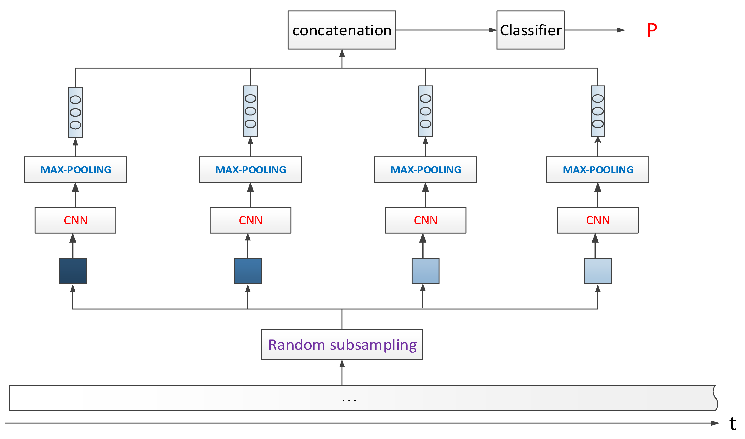
Our first model, CNN_Random_Agg, in short, is based on this kind of random block/sentence sub-sampling, and then aggregates the extracted local CNN features for classification. This model is shown in Figure 1. Input X is a word vector matrix of n × d, where n is the word number of the full document and d is the dimension of the word vector. We first randomly sample a few groups of words in the full document range as with w words in each group, where is the sampled block of words with the size of , and K is the number of sampled groups. In our experiments, just 6–10% of the full document words could obtain good performance. Then, we use 1d-CNN, Relu (Rectified Linear Unit) activation function, and max-pooling operation to extract the features of each group as follows:
Here, Conv1D is the 1d CNN operator and W is the tensor of the convolutional filters with the shape of , where h is convolutional kernel size, d is the dimension of the word vector same as above, and f is the number of convolutional filters. Thus, after the operation of Equation (1), , the convoluted feature for each group, is further pooled to by the max over time pooling operation as Equation (2). Then, for the K sampled groups of words, the extracted local CNN features are concatenated as follows:
This aggregated CNN feature y is then input to the last full-connected layer for classification. Finally, we perform the Softmax operation and output the probability p.
3.2. Model_2: CNN Feature with LSTM Aggregation
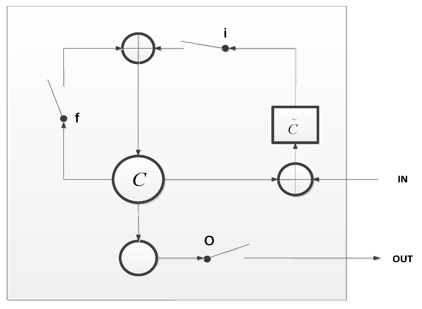
In the first model, we extracted and aggregated local CNN features from the randomly sampled blocks or sentences of the document for classification. This kind of feature aggregation is simple and effective, though the correlation among those sampled blocks is lost. This is because there is no order information between the randomly sub-sampled blocks, which results in less semantic association between the feature vectors of these blocks. Therefore, we consider using a recurrent neural network (RNN) to explicitly model the semantic order of the sampled blocks. RNNs have shown great success in many NLP tasks, such as non-segmented continuous handwriting recognition [21] and autonomous speech recognition [22]. Specifically, in this model we use LSTM [15] nodes as RNN computational nodes, shown in Figure 2. The advantage of the LSTM node is that it well tackles the difficulty of “gradient vanishing” and “gradient exploding” by its carefully designed gates. Therefore, it is possible to design a deeper LSTM network and unfold this network into many steps, which is suitable for practical sequential data modeling.
The LSTM node is calculated as follows [15]:
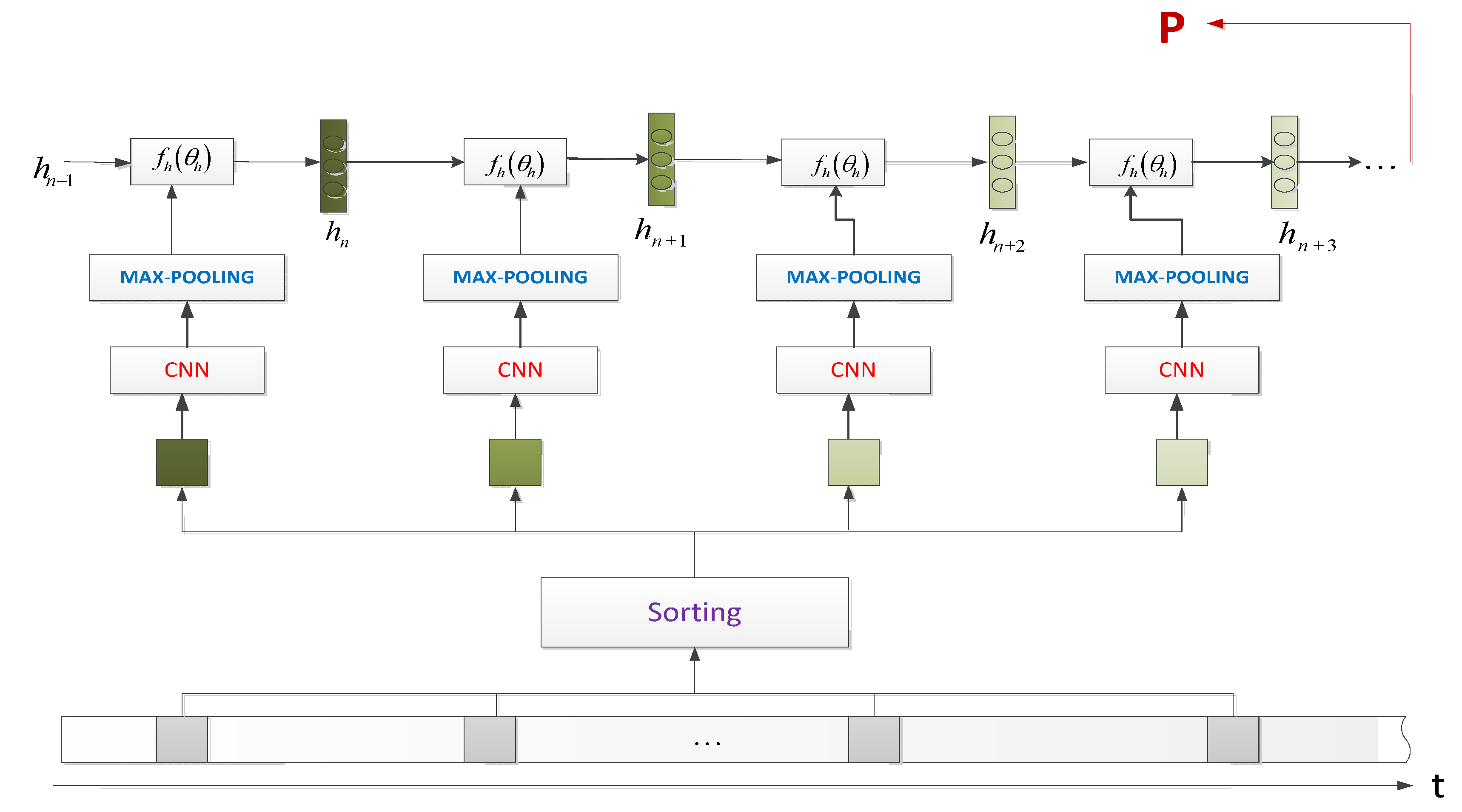
In our second model, CNN_LSTM_Agg, in short, we sorted each group of words in the order of text to obtain the semantic order, so as to form a set of ordered document data. The first steps are the same as the model of CNN_Random_Agg, but the key difference to the model of CNN_LSTM_Agg is that we use an LSTM layer to aggregate the extracted local CNN features for classification. The specific model structure is shown in Figure 3.
3.3. Model_3: CNN Feature with Recurrent Attention Model
In the previous two models, we use the random sub-sampling technique to extract parts of the text. As a result, the blocks of words that the two models selected are purely random, which do not represent the most salient parts of the document. In view of this, we consider introducing a smart sampling agent that can quickly find the best positions for those blocks. Inspired by the seminal recurrent attention model (RAM) [9], we expect to employ reinforcement learning to control the locations of sampled blocks, so that we could select more suitable blocks of words that better represent the characteristics of the document.
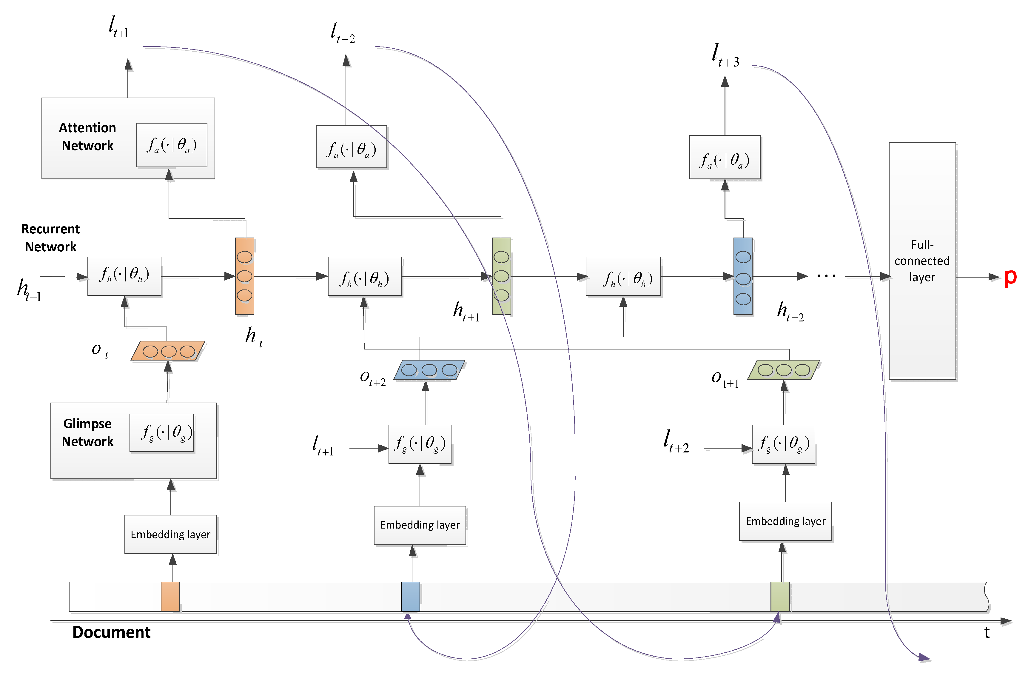
The diagram of the model CNN_RAM_Agg is shown in Figure 4. This document classification framework incorporates the recurrent attention mechanism, which includes a glimpse network module for local CNN feature extraction, a recurrent neural network module for CNN feature aggregation, and an attention network for sampling location predication. The algorithm of this model is shown in Algorithm 1.
| Algorithm 1: CNN_RAM_Agg |
| 1: Input: Document D, GloVe dictionary, initial network parameter ( for attention network, for recurrent network, for glimpse network), number of glimpse T, maximum iteration maxIter. 2: for i = 0, 1, 2, …, maxIter do 3: for t = 0, 1, 2, … T do ( is initialized by a random location) Extract words near the position and use GloVe to obtain the word vectors Use the glimpse network to extract feature vectors Input to the LSTM network to obtain a new hidden state Predict the next location by the attention network with 4: end for 5: Using the aggregated feature emitted from the last step of LSTM to obtain the predicted label. 6: If predicted label is correct then get reward 1 otherwise get none reward. 7: Update parameters with reinforcement learning; update parameters and parameter with back propagation 8: end for |
Following the mechanism of RAM [9], at the glimpse step, the location is predicted by the attention network of previous step. Then, a block of words is extracted near this location and the local CNN features are extracted by the glimpse network . Next, is aggregated with the previous hidden state to obtain a new hidden state by the LSTM network . Then, the attention network predicts the next location for the next glimpse step. After the model glimpses T locations, the last state of LSTM is used for document classification. Note that we use a reinforcement learning technique to train the attention network because the predicted location is not differentiable with respect to . Thus, if the predicted label is correct, our model receives reward , otherwise . Then, the attention network is optimized by maximizing the expected cumulative return, as Equation (5):
where is the optimized policy, which predicts the next position according to its glimpse at each step; is the reward for each step; and R is the cumulative return, which is defined as follows:
where is the decaying coefficient.
4. Experiment Analysis
This section mainly introduces the data set used for the experiment, the experimental setup, and the comparative analysis of the experimental results.
4.1. Data Set
We collected four classes of papers from arXiv as the benchmark dataset for long document classification. They are cs.IT, cs.NE, math.AC, and math.GR, and the number of papers in each class is 3233, 3012, 2885, and 3065, respectively. Among them, each class in our dataset has an average of more than 6000 words, which is much longer than other short document datasets, such as IMDb (Internet Movie Database) reviews, Amazon reviews, and so on.
Because the format of these papers is very special, we take the following preprocessing steps. First of all, as the texts of each paper are converted from PDF format, in order to remedy the side effect to classification, we have to remove the garbled characters, punctuation, and numbers in the paper because they are missing in GloVe [23]. Next, we convert the document into a long string and a typical word segmentation operation is performed on the string to get a long list of words. Finally, the list of words ar1 converted into word vectors through the GloVe dictionary. For those words that are not in GloVe, we use random word vectors as a supplement, which can be further trained by our model. The details of the data are shown in Table 1.
4.2. Experiment Setup
- Experiment platform: The experimental platform is a deep learning workstation with 32 Gb RAM and NVIDIA Titan X GPU with 12 Gb memory. The computer is installed with Ubuntu16.04 system and the program mentioned in the experiment is implemented with TensorFlow 1.8 [24].
- Word vector: The word vector used in this article is GloVe. GloVe originally stored 400,000 word vectors, but there are around 730,000 missing words in our arXiv dataset. Then, the number of the final embedding lookup word vector table is around 1.13 million. Therefore, if we use a 300-dimension word vector, we cannot store the lookup table in GPU memory. For this reason, we chose to use a 100-dimension word vector.
- Training parameters: In the experiment, we set 5000 steps, and we used Adam’s optimization method to train our model. The learning rate was set to 0.001, and it gradually became 0.0001. Dropout’s coefficient is set to 0.5. The input batch size is 64. For the convolution layer, convolution kernels with convolution kernel sizes 3, 4, and 5 are used, with 128 convolution kernels of each size.
4.3. Experiment Results
4.3.1. Baseline Model
We used the popular CNN model proposed in the literature [3] as the baseline method for our experiments. As the document in the arXiv dataset is too long to be directly used by the CNN baseline model, each document is trimmed to its first 1000 words. Based on the same hyper-parameter setting in the literature [3], the classification result on the arXiv dataset is 91.94%. This result is plotted in Figure 5a,b as the baseline for comparison.
4.3.2. Model 1: CNN_Random_Agg
For model CNN_Random_Agg, we performed the following experiments by changing two parameters: window size and total number of words. The experimental results are shown in Table 2.
From the above table, we can see that when the window size is fixed, total number of words extracted is higher; that is, the more blocks that are sub-sampled, the better the experimental results. Because the total number of words extracted determines the ratio of the full-text content that the model can see, the more it sees, the more useful information it contains, resulting in better classification results. On the other hand, when the extracted total number of words is fixed, the larger the window size, the better the experimental results. Because the words in a window have closer local correlation, their relevance is large.
4.3.3. Model 2: CNN_LSTM_Agg
For model CNN_ LSTM _Agg, we performed the following experiments by changing the three parameters: window size, total number of words, and number of hidden unit. For each fixed window size and total number of words, the result for the 256 hidden unit is at the top and 512 is at the bottom. The experimental results are shown in Table 3.
From Table 3, we can see that the accuracy increases gradually with the increase of the window size and the total number of words. When the window size is 10 and the total number of words is 200, that is, the number of blocks extracted is 20, the accuracy is only about 88%; and when the total number of words increases to 1000 and the window size increases to as large as 200, that is, the number of blocks is 5, the accuracy of the model reached more than 94%. In addition, we also investigate the effect of the number of hidden units by setting the number to 256 and 512, respectively. Experiments show that setting hidden units to 256 is better than the case of 512. This may because the current collected arXiv dataset is still too small relative to a larger RNN network, which could be easily overfit. We hope to enlarge our dataset in future work.
4.3.4. Model 3: CNN_RAM_Agg
For model CNN_RAM_Agg, we also performed experiments based on the two parameters of window size and total number of words, the experimental results are shown in Table 4.
From Table 4, we can see that different from CNN_Random_Agg and CNN_LSTM_Agg, CNN_RAM_Agg achieves its best accuracy not with the largest window size, but with a suitable window size. When we extract 1000 words and the window size is 200, that is, by taking 5 glimpses, the accuracy reaches 95.48%. This result is higher than the first two models. This fully demonstrates that the RAM model is very suitable for the long length document scenario.
4.3.5. Experimental Comparison
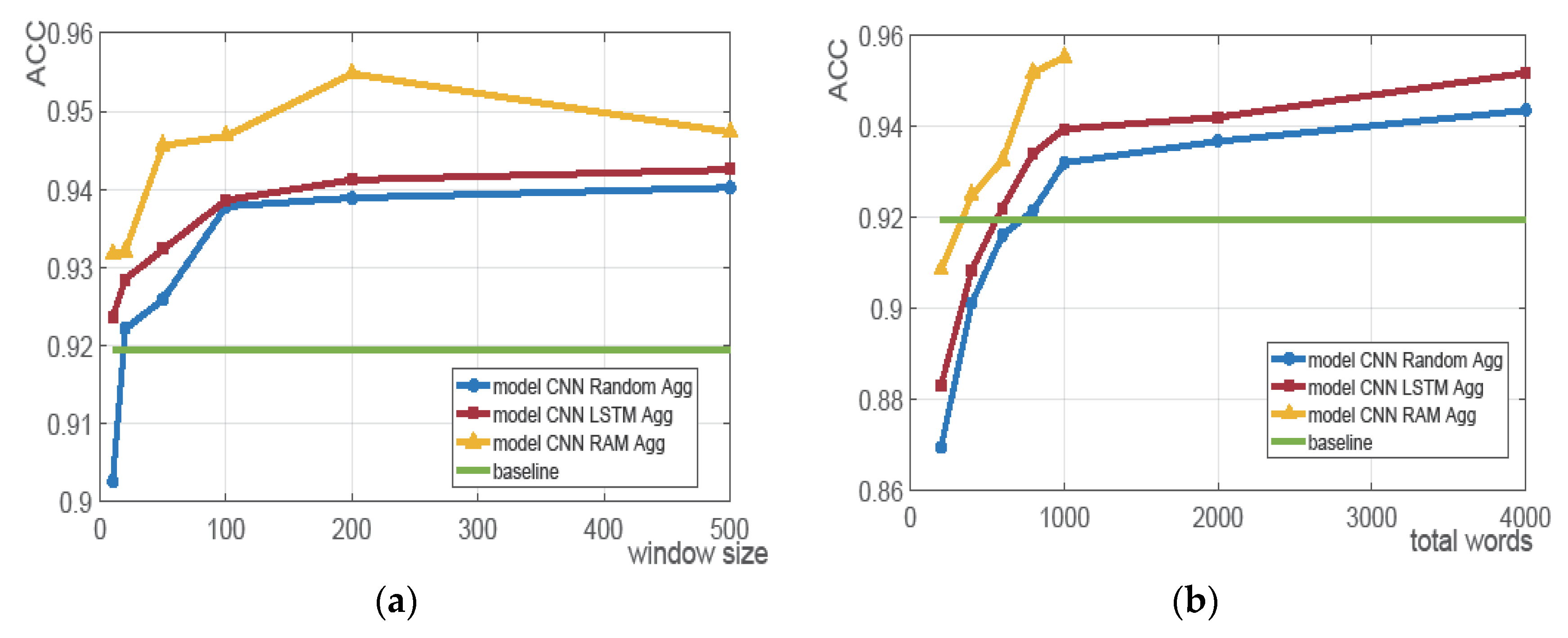
We compared the experimental results of the three proposed models and the baseline model. The comparison is shown in Figure 5. We can clearly see that the results of our proposed models are superior to the baseline with proper setting. In Figure 5a, because the baseline model only exploited the first 1000 words in a document, for fair comparison, we fixed the number of extracted words to 1000 and varied the window size for the three proposed models. Both CNN_LSTM_Agg and CNN_RAM_Agg outperform the baseline by a large margin for all windows size settings. CNN_Random_Agg is also superior to the baseline except that the window size was set to 10. Moreover, in Figure 5b, we can observe that even with much fewer extracted words, the proposed sub-sampling methods can beat the baseline. In particular, CNN_RAM_AGG outperforms the baseline with less than 400 words. It is not surprising that the sub-sampling methods are superior to the classic CNN baseline, because the CNN baseline is limited to the first 1000 words because of memory constraints. On the contrary, these sub-sampling based methods make use of the full coverage.
To investigate the performance of these sub-sampling approaches, we first varied the window size from 10 to 500 while fixing the total number of words to 1000. The results are shown in Figure 5a. It can be observed that the classification accuracy of the three models gradually increases as the size of the window increases. However, for CNN_RAM_Agg, there is an interesting decrease when setting window size from 200 to 500. This is because the total number of extracted words is only 1000, then the window size of 500 means CNN_RAM_Agg can only glimpse two word blocks, but for the window size of 200 CNN_RAM_Agg, can glimpse five word blocks. In some sense, more word blocks may cover more global information, which increases the possibility of it focusing on other salient parts.
Secondly, by fixing the window size to 40, we increased the total number of extracted words from 200 to 4000. Note that for CNN_RAM_Agg, we only extracted up to 1000 words. Figure 5b demonstrates that CNN_RAM_Agg significantly outperforms the other two models with the least information. Even with 200 extracted words, say only 3% of the average words are used, CNN_RAM_Agg can achieve more than 90% classification accuracy. Moreover, by glimpsing 20 blocks, say extracting 1000 words, CNN_RAM_Agg is still superior to CNN_Random_Agg and CNN_LSTM_Agg, which have seen 4000 words. It definitely shows that the RAM mechanism is well trained and can smartly locate the most salient blocks of words for long length document.
Even though CNN_RAM_Agg outperforms CNN_Random_Agg and CNN_LSTM_Agg with least extracted words, CNN_RAM_Agg requires much more training time than these two approaches. Besides less training time, CNN_Random_Agg and CNN_LSTM_Agg are easy to implement. Additionally, compared with the classical CNN baseline model, these two methods aggregate the local CNN word features in the full coverage to produce superior results for long document classification.
5. Conclusions
This paper introduces three sub-sampling based models for long document classification, using convolutional neural networks, recurrent neural networks, and a recurrent attention model. The experimental analysis shows that our models can perform document classification tasks well even with incomplete information. Among these models, the RAM based model can effectively and quickly find the statement that best characterizes the text feature in the long document. We only need to use less than 10% of the document text to achieve good results. For the classification of long documents, we have greatly reduced the computational complexity and memory requirement, which is easy for deployment in practice.
Author Contributions
L.L., K.L. and Z.C. conceived and designed the experiments; J.Z. and L.L. performed the experiments; Y.J. and J.H. analyzed the data; L.L. and J.H. wrote the paper with contributions from all authors. All authors read and approved the submitted manuscript, agreed to be listed, and accepted this version for publication.
Funding
This work is supported by STATE GRID Corporation of China Headquarters Technology Program 2017.
Conflicts of Interest
The authors declare no conflict of interest.
References
- Wang, S.; Manning, C.D. Baselines and bigrams: Simple, good sentiment and topic classification. In Proceedings of the 50th Annual Meeting of the Association for Computational Linguistics: Short Papers-Volume 2, Jeju Island, Korea, 8–14 July 2012; Association for Computational Linguistics: Stroudsburg, PA, USA, 2012; pp. 90–94. [Google Scholar]
- Pang, B.; Lee, L. Seeing stars: Exploiting class relationships for sentiment categorization with respect to rating scales. In Proceedings of the 43rd Annual Meeting on Association for Computational Linguistics, Ann Arbor, MI, USA, 25–30 June 2005; Association for Computational Linguistics: Stroudsburg, PA, USA, 2005; pp. 115–124. [Google Scholar]
- Kim, Y. Convolutional Neural Networks for Sentence Classification. Eprint Arxiv 2014, arXiv:1408.5882. [Google Scholar]
- Lai, S.; Xu, L.; Liu, K.; Zhao, J. Recurrent Convolutional Neural Networks for Text Classification. In Proceedings of the Twenty-Ninth AAAI Conference on Artificial Intelligence, Austin, TX, USA, 25–30 January 2015; Volume 333, pp. 2267–2273. [Google Scholar]
- Yang, Z.; Yang, D.; Dyer, C.; He, X.; Smola, A.; Hovy, E. Hierarchical attention net-works for document classification. In Proceedings of the NAACL-HLT, San Diego, CA, USA, 12–17 June 2016; pp. 1480–1489. [Google Scholar]
- Zhang, X.; Zhao, J.; Lecun, Y. Character-level Convolutional Networks for Text Classification. In Proceedings of the NIPS’15 28th International Conference on Neural Information Processing Systems, Montreal, QC, Canada, 7–12 December 2015; pp. 649–657. [Google Scholar]
- Tang, D.; Qin, B.; Liu, T. Document Modeling with Gated Recurrent Neural Network for Sentiment Classification. In Proceedings of the Conference on Empirical Methods in Natural Language Processing, Lisboa, Portugal, 17 September 2015; pp. 1422–1432. [Google Scholar]
- Hu, M.; Liu, B. Mining and summarizing customer reviews. In Proceedings of the Tenth ACM SIGKDD International Conference on Knowledge Discovery and Data Mining, Seattle, WA, USA, 22–25 August 2004; pp. 168–177. [Google Scholar]
- Mnih, V.; Heess, N.; Graves, A. Recurrent models of visual attention. In Proceedings of the Advances in Neural Information Processing Systems, Montreal, QC, Canada, 8–13 December 2014; pp. 2204–2212. [Google Scholar]
- Simonyan, K.; Zisserman, A. Very deep convolutional networks for large-scale image recognition. arXiv 2014, arXiv:1406.6247. [Google Scholar]
- Szegedy, C.; Liu, W.; Jia, Y.; Sermanet, P.; Reed, S.; Anguelov, D.; Erhan, D.; Vanhoucke, V.; Rabinovich, A. Going deeper with convolutions. In Proceedings of the IEEE Conference on Computer Vision and Pattern Recognition, Boston, MA, USA, 7–12 June 2015; pp. 1–9. [Google Scholar]
- He, K.; Zhang, X.; Ren, S.; Sun, J. Deep Residual Learning for Image Recognition. In Proceedings of the 2016 IEEE Conference on Computer Vision and Pattern Recognition (CVPR), Las Vegas, NV, USA, 27–30 June 2016; pp. 770–778. [Google Scholar]
- Maas, A.L.; Daly, R.E.; Pham, P.T.; Huang, D.; Na, A.Y.; Potts, D. Learning word vectors for sentiment analysis. In Proceedings of the 49th Annual Meeting of the Association for Computational Linguistics: Human Language Technologies-Volume 1, Portland, OR, USA, 19–24 June 2011; Association for Computational Linguistics: Stroudsburg, PA, USA, 2011; pp. 142–150. [Google Scholar]
- Nguyen, T.H.; Grishman, R. Relation Extraction: Perspective from Convolutional Neural Networks. In Workshop on Vector Modeling for NLP; Blunsom, P., Cohen, S., Dhillon, P., Liang, P., Eds.; Association for Computational Linguistics: Stroudsburg, PA, USA, 2015; pp. 39–48. [Google Scholar]
- Hochreiter, S.; Schmidhuber, J. Long short-term memory. Neural Comput. 1997, 9, 1735–1780. [Google Scholar] [CrossRef] [PubMed]
- Sutskever, I.; Vinyals, O.; Le, Q.V. Sequence to Sequence Learning with Neural Networks. In Proceedings of the 27th International Conference on Neural Information Processing Systems, Montreal, QC, Canada, 8–13 December 2014; Volume 4, pp. 3104–3112. [Google Scholar]
- Bahdanau, D.; Cho, K.; Bengio, Y. Neural Machine Translation by Jointly Learning to Align and Translate. arXiv 2014, arXiv:1409.0473. [Google Scholar]
- Nallapati, R.; Zhou, B.; dos Santos, C.; Gulcehre, C.; Xiang, B. Abstractive Text Summarization Using Sequence-to-Sequence RNNs and Beyond. arXiv 2016, arXiv:1602.06023. [Google Scholar]
- Wang, Z.; He, W.; Wu, H.; Wu, H.; Li, W.; Wang, H.; Chen, E. Chinese Poetry Generation with Planning based Neural Network. arXiv 2016, arXiv:1610.09889. [Google Scholar]
- Liu, P.; Qiu, X.; Huang, X. Recurrent neural network for text classification with multi-task learning. arXiv 2016, arXiv:1605.05101. [Google Scholar]
- Graves, A.; Liwicki, M.; Fernández, S.; Bertolami, R.; Bunke, H.; Schmidhuber, J. A novel connectionist system for unconstrained handwriting recognition. IEEE Trans. Pattern Anal. Mach. Intell. 2009, 31, 855–868. [Google Scholar] [CrossRef] [PubMed]
- Miao, Y.; Gowayyed, M.; Metze, F. EESEN: End-to-end speech recognition using deep RNN models and WFST-based decoding. In Proceedings of the 2015 IEEE Workshop on Automatic Speech Recognition and Understanding (ASRU), Scottsdale, AZ, USA, 13–17 December 2015; pp. 167–174. [Google Scholar]
- Pennington, J.; Socher, R.; Manning, C. Glove: Global Vectors for Word Representation. In Proceedings of the 27th Conference on Empirical Methods in Natural Language Processing, Doha, Qatar, 25–29 October 2014; pp. 1532–1543. [Google Scholar]
- Tensorflow. Available online: https://github.com/tensorflow/tensorflow (accessed on 23 July 2018).
- Stra, J.; Bengio, Y. Random search for hyper-parameter optimization. J. Mach. Learn. Res. 2012, 13, 281–305. [Google Scholar]
- Snoek, J.; Larochell, H.; Adams, R.P. Practical bayesian optimization of machine learning algorithms. In Proceedings of the Advances in neural information processing systems, Lake Tahoe, NV, USA, 3–6 December 2012; pp. 2951–2959. [Google Scholar]
Figure 1.
Model convolutional neural networks (CNN)_Random_Agg architecture.

Figure 2.
Long–short term memory (LSTM) node.

Figure 3.
Model CNN_LSTM_AGG architecture.

Figure 4.
Model CNN_RAM_Agg architecture. RAM—recurrent attention model.

Figure 5.
Experimental results of these models (ACC is the accuracy of classification): (a) Fixing the number of extracted words to 1000, vary the window size; (b) Fixing the window size to 40 words, vary the total number of extracted words.
Figure 5.
Experimental results of these models (ACC is the accuracy of classification): (a) Fixing the number of extracted words to 1000, vary the window size; (b) Fixing the window size to 40 words, vary the total number of extracted words.


Table 1.
Data statistics: #w denotes the number of words (maximum, minimum, and average per document).
Table 1.
Data statistics: #w denotes the number of words (maximum, minimum, and average per document).
| Class Name | Number of Documents | Average Words |
|---|---|---|
| cs.IT | 3233 | 5938 |
| cs.NE | 3012 | 5856 |
| math.AC | 2885 | 5984 |
| math.GR | 3065 | 6642 |
Table 2.
Model CNN_Random_Agg experimental results.
| Window Size | 10 | 20 | 50 | 100 | 200 | 400 | 500 | |
|---|---|---|---|---|---|---|---|---|
| Total Words | ||||||||
| 200 | 86.37% | 86.53% | 86.98% | 87.03% | 87.21% | |||
| 400 | 87.48% | 90.11% | 90.33% | 90.60% | 92.08% | 92.12% | ||
| 600 | 88.36% | 91.21% | 91.88% | 92.16% | 93.35% | |||
| 800 | 89.14% | 92.13% | 92.32% | 92.63% | 93.38% | 93.41% | ||
| 1000 | 90.26% | 92.21% | 92.59% | 93.78% | 93.89% | 94.02% | ||
Table 3.
Model CNN_LSTM_Agg experimental results.
| Window Size | 10 | 20 | 50 | 100 | 200 | 400 | 500 | |
|---|---|---|---|---|---|---|---|---|
| Total Words | ||||||||
| 200 | 88.16% | 88.21%% | 90.67% | 90.96% | 91.32% | |||
| 83.42% | 86.05% | 86.71% | 87.23% | 88.06% | ||||
| 400 | 89.05% | 91.03% | 91.35% | 91.62% | 92.21% | 92.33% | ||
| 86.28% | 88.41% | 89.08% | 89.27% | 90.08% | 90.12% | |||
| 600 | 89.52% | 91.96% | 92.03% | 92.85% | 93.87% | |||
| 86.66% | 89.59% | 89.92% | 90.23% | 90.51% | ||||
| 800 | 90.28% | 92.41% | 93.12% | 93.32% | 94.01% | 94.35% | ||
| 89.44% | 90.28% | 90.37% | 90.56% | 90.82% | 90.94% | |||
| 1000 | 92.36% | 92.85% | 93.23% | 93.86% | 94.12% | 94.25% | ||
| 89.48% | 90.36% | 90.61% | 91.77% | 91.96% | 92.34% | |||
Table 4.
Model CNN_RAM_Agg experimental results.
| Window Size | 10 | 20 | 50 | 100 | 200 | 400 | 500 | |
|---|---|---|---|---|---|---|---|---|
| Total Words | ||||||||
| 200 | 89.84% | 90.15% | 91.67% | 91.89% | 92.23% | |||
| 400 | 90.05% | 92.22% | 93.08% | 93.56% | 93.67% | 93.53% | ||
| 600 | 90.11% | 92.38% | 93.68% | 94.24% | 94.11% | |||
| 800 | 92.36% | 92.53% | 93.86% | 94.36% | 94.41% | 93.87% | ||
| 1000 | 93.17% | 93.21% | 94.56% | 94.68% | 95.48% | 94.73% | ||
© 2018 by the authors. Licensee MDPI, Basel, Switzerland. This article is an open access article distributed under the terms and conditions of the Creative Commons Attribution (CC BY) license (http://creativecommons.org/licenses/by/4.0/).
Share and Cite
MDPI and ACS Style
Liu, L.; Liu, K.; Cong, Z.; Zhao, J.; Ji, Y.; He, J. Long Length Document Classification by Local Convolutional Feature Aggregation. Algorithms 2018, 11, 109. https://doi.org/10.3390/a11080109
AMA Style
Liu L, Liu K, Cong Z, Zhao J, Ji Y, He J. Long Length Document Classification by Local Convolutional Feature Aggregation. Algorithms. 2018; 11(8):109. https://doi.org/10.3390/a11080109
Chicago/Turabian StyleLiu, Liu, Kaile Liu, Zhenghai Cong, Jiali Zhao, Yefei Ji, and Jun He. 2018. "Long Length Document Classification by Local Convolutional Feature Aggregation" Algorithms 11, no. 8: 109. https://doi.org/10.3390/a11080109
Note that from the first issue of 2016, this journal uses article numbers instead of page numbers. See further details here.