A Weighted Histogram-Based Tone Mapping Algorithm for CT Images
by
 , , and
David Völgyes
1,* ,
,
Anne Catrine Trægde Martinsen
2,3,
Arne Stray-Pedersen
4,5,
Dag Waaler
6 and
Marius Pedersen
7 1
Department of Computer Science, Norwegian University of Science and Technology, 2815 Gjøvik, Norway
2
Department of Physics, University of Oslo, 0316 Oslo, Norway
3
Department of Diagnostic Physics, Oslo University Hospital, 0424 Oslo, Norway
4
Department of Forensic Sciences, Oslo University Hospital, 0424 Oslo, Norway
5
Institute of Clinical Medicine, University of Oslo, 0318 Oslo, Norway
6
Department of Health Sciences in Gjøvik, Norwegian University of Science and Technology, 2803 Gjøvik, Norway
7
Department of Computer Science, Norwegian University of Science and Technology, 2815 Gjøvik, Norway
*
Author to whom correspondence should be addressed.
Algorithms 2018, 11(8), 111; https://doi.org/10.3390/a11080111
Submission received: 16 June 2018
/
Revised: 16 July 2018
/
Accepted: 20 July 2018
/
Published: 25 July 2018
Abstract
:Computed Tomography (CT) images have a high dynamic range, which makes visualization challenging. Histogram equalization methods either use spatially invariant weights or limited kernel size due to the complexity of pairwise contribution calculation. We present a weighted histogram equalization-based tone mapping algorithm which utilizes Fast Fourier Transform for distance-dependent contribution calculation and distance-based weights. The weights follow power-law without distance-based cut-off. The resulting images have good local contrast without noticeable artefacts. The results are compared to eight popular tone mapping operators.
1. Introduction
Global and local contrasts are often imperfect in images. The available dynamic range of the display is either not utilized, or, on the contrary, the range is wider than the low dynamic range display.
Medical images, particularly Computed Tomography (CT) images, are challenging to visualize. First, artefacts could lead to inferior diagnostic performance [1]. Second, a lack of good local contrast could also limit diagnostic performance; local contrast enhancement can improve diagnostic efficiency [2] or significantly reduce interpretation times [3]. Third, CT images have low soft tissue contrast, a relatively high noise level compared to magnetic resonance imaging (MRI), and they have a high dynamic range (approximately 12 bits) [4].
CT images represent absolute tissue densities using CT numbers that are measured in Hounsfield units (HU) [5]. This calibrated nature of the CT imaging makes it appealing to use global, monotonic tone mapping operators (TMO) which assign the same color to pixels representing the same tissue density, regardless of the location of the pixels.
Specialized protocols are developed for diagnosing specific pathologies. However, the need for image post-processing in order to obtain better local contrast [6,7,8] dates back decades.
In the following, we briefly overview the most important approaches for global and local contrast enhancement approaches for CT images before we present our proposed local method.
1.1. Histogram Methods
Histogram equalization [9] is one of the simplest contrast adjusting algorithms, and it has been applied to CT images since the mid-1980s [6]. The main idea is that every shade available should be used for approximately the same number of pixels. Assuming N different shades, the frequency of a shade is then:
Histogram equalization is a kind of maximum-entropy approach because Shannon-entropy Equation (2) has its maximum when the probabilities are equal:
Brightness is assigned to a given shade using, F, the cumulative distribution function of the pixel values and U as the cumulative distribution function of a uniform distribution:
While histogram equalization has some very useful properties, it does not guarantee good local contrast. One approach could be to minimize normalized Shannon information distance between the source distribution and the displayed image, which is the basis of the CT windowing algorithm from Nikvand et al. [10]. Despite its adaptive nature, this algorithm belongs to the global operators, and might not yield good local contrast, and its generalization seems to be non-trivial.
Local histogram equalization (LHE) [11] is meant to solve the problem of local contrast using a sliding window histogram and equalizing the local histograms. This algorithm could over-amplify local noise, especially for homogeneous regions which are larger than the window size. Contrast-limited adaptive histogram equalization (CLAHE) [7] uses an upper limit for the histogram bins. If a bin has higher counts than this number, the peak is truncated at the limit, and the extra counts are distributed to all of the bins uniformly. This effectively prevents high peaks in the histogram from over-stretching. In the case of an extremely small limit, all of the bins become truncated, and then the cut area is redistributed uniformly, which leads to a flat histogram. However, CLAHE has a limited window size which leads to halos, while larger windows limit the locality and adaptiveness of the algorithm.
Not only spatial adaptation, but also histogram processing is the subject of intensive research. The contrast limitation in CLAHE can be seen as an early approach. Another approach could be splitting the histogram into two or more parts, and equalizing them into pre-determined ranges. This technique is known as bi-histogram equalization [12]. This ensures that every important part of the histogram gets enough dynamic range. For instance, in CT images, the histogram could be split into three parts, representing lung tissue, soft tissues, and bones.
A generalized form is prescribing the shape of the histogram [13], using cumulation functions [14], or requiring the extreme of a mapping descriptor, for instance, the above-mentioned normalized information distance [10].
One of the most appealing features of the histogram-based methods is the fact that the individual processing methods could be combined easily. For instance, the CLAHE algorithm could easily be combined with the bi-histogram equalization approach.
1.2. Tone Mapping
CT images are often windowed, which means that only part of the dynamic range is displayed, and this part is processed with histogram equalization-based methods.
The problem can be seen as a high dynamic range imaging issue: the high dynamic range CT image should be tone mapped to be displayed on a low dynamic range display while preserving local contrast.
High dynamic range images are often processed with tone mapping operators to keep or enhance local contrast while compressing the dynamic range, to fit into the displaying medium’s dynamic range.
Besides histogram equalization, the simplest dynamic range compression algorithm is gamma compression which maps source image intensity to a target image intensity in the following way:
where , I are the source and target images, respectively. and are used to refer to the pixel values of these images.
While this effectively reduces the dynamic range if , it does not ensure good local contrast. A popular choice to keep or increase local contrast is the base layer—detail layer separation. The base layer (B) of an image consists of larger structures and has a high dynamic range, while the detail layer (D) is the difference between the original image () and the base layer:
Any filter which removes small details could be used for this separation, including a Gaussian filter, and edge preserving denoising filters (median, total variation minimization, bilateral filter, among others).
After the dynamic range compression of the base layer, the details should be added back using a scale factor () and can even be enhanced. This could be simple multiplication (), or more sophisticated edge enhancement where the detail layer is pre-processed before it is combined with the compressed base layer into a tone mapped image (TMI):
This base-detail layer separation technique is the basis of numerous algorithms. Using a Gaussian filter for detail separation and leaving the base layer uncompressed yields the unsharp masking algorithm, which belongs to the wider class of local contrast enhancement techniques. Applying any compression on the base layer, even simple linear rescaling, yields a tone mapping algorithm. The approach can be generalized into multi-layer separation using linear [15] or nonlinear decomposition [16]. The quality of these approaches depends on the separation filter and the base layer compression. One very active research area is to find good, edge preserving filters avoiding such artefacts. For instance, the following filters were proposed for base-detail separation: Gaussian filter, anisotropic diffusion, weighted least squares (WLS) [16], total variation (TV) based filters using [17] and [18] norms and bilateral filter [19], among others. While this separation is more like a framework than an algorithm, it is an important building block of tone mapping operators and detail manipulation algorithms.
Besides the layer separation approach, many other tone mapping approaches have been developed. Reinhard’02 operator simulates the effect of photographic zones with an additional dodging-and-burning step [20]. Fattal’s approach [21] is based on gradient attenuation. The smaller than threshold gradients are slightly magnified while larger gradients are suppressed. The attenuated gradients lead to a Laplace–Poisson problem which can be solved iteratively. Mantiuk presented a perceptual framework for contrast processing, which is related to the gradient suppression approach but models perceptual contrast. This is not the only way to model the human visual system (HVS). Drago’s method is built on the logarithmic compression of luminance values [22], and the Reinhard’05 [23] operator models the photoreceptor adaptation on local and global levels. The approach by Ferradans et al. [24] models visual adaptation for global tone mapping which is followed by a second stage local contrast enhancement. The Mantiuk’08 operator [25] iteratively minimizes the visible distortion of the image measured by an error metric, and takes into account both the display properties and the properties of HVS. Color perception plays a central role in retinex-based TMO [26] and in the so-called iCAM model which is a ‘next-generation color appearance model’ [27]. For further details, we refer the interested reader to the literature [28,29].
Our proposed method builds on spatially weighted histogram equalization. It can be seen as an effective tone mapping approach or as a method for local contrast enhancement. Our aim was to avoid halos and artefacts of local histogram methods and ensure good local contrast. While histogram methods have been used for medical image processing since the 1980s, the effectiveness of tone mapping operators has also been demonstrated on medical images, for instance Fattal’s method [21].
The literature on histogram methods and tone mapping operators is vast; further details can be found, for instance, in [30].
2. Problem Statement
Good local contrast has a very important role in computed tomography (CT) images used for diagnosing pathologies [31]. Unlike traditional photographs, CT images contain a measurement of material densities, and these are unaffected by irradiation. Traditional tone mapping assumes that the image is the product of illumination and reflectance [32].
CT images also have huge dynamic range, and a global histogram equalization would not yield good enough local contrast, while local methods might yield unwanted halos. Our main goal is to develop an algorithm which is able to compress high dynamic range images into a low dynamic range while presenting as much local information as possible, preserving the main structures, not exhibiting strong halos, and more or less keeping pixel intensity ordering.
Theoretically, any tone mapping operator could be used for medical images. However, the required contrast strongly depends on the tissue, and the absolute contrast is the smallest for medium CT densities, for instance kidney (20–45 HU), muscle (35–55 HU) [33], while the absolute contrast is large for small CT densities, for instance gas volumes (−1000 HU) and lung tissue (−700–500 HU) [34] and also large for dense parts, such as calcification (>150 HU) and bones [35]. Traditional tone mapping operators do not necessarily perform well for these regions, global histogram equalization lacks locality, while local histogram equalization methods (LHE/CLAHE) often lead to halos.
In practical terms, the aim of this paper is to develop a local tone mapping operator which lies somewhere between global and local histogram equalization and combines their advantages and avoids their shortcomings.
3. Theory
The main drawback of local histogram equalization methods is the often visible halos around strong edges. This issue originates from the limited size of the locality window. However, applying a large window limits the locality of the method, and gradually converges towards a global method, while it requires more computational power. Using adjacent or slightly overlapping blocks instead of sliding windows could effectively reduce the required resources, but could lead to blocking artefacts.
Our approach is built on the following ideas:
- Local neighborhood is important in order to determine a given pixel’s intensity.
- Neighborhood should not have a strong cut-off; the weighted contribution of the whole image should be taken into account.
- The contribution is a decreasing function of the distance.
- The contribution can be calculated using a Fast Fourier transform (FFT) [36].
- The intensity of the pixel is determined based on the local relative intensities in the source image.
- Locality and noise tolerance are equally important.
The concept of using convolution to calculate the sliding window local histogram was established decades ago [11]. Initially, the rectangular window function was used; later, this was generalized to other shapes and functions. However, to the best of our knowledge, the weighting function always had a cut-off, either determined by the window size, or by the fast decreasing weights, such as Gaussian weighting.
We argue that a power function should be used as the weighting function for two reasons. First, according to Blommaert [37], normalized local contributions to perceived brightness follow a power-law with a negative exponent:
Using this function family means that our proposed algorithm uses a similar weighting approach as the human visual system.
Second, intuitively, this function shape is required for good local contrast without creating halos: if the function does not decrease fast enough, the weighting will resemble a global histogram equalization and will not sufficiently prioritize local information. On the other hand, if the weighting function has a small effective kernel, either because of the window size, or because of the too fast decreasing weights, then the further lying pixels will not contribute enough to the local histograms which leads to halos around sharp edges. However, this effect can be controlled using contrast stretching limitations, such as in CLAHE.
The FFT-based contribution calculation [11] and contrast-limited equalization [7] are known methods, but they are important for the proposed algorithm, and are thus briefly reviewed in the following sections.
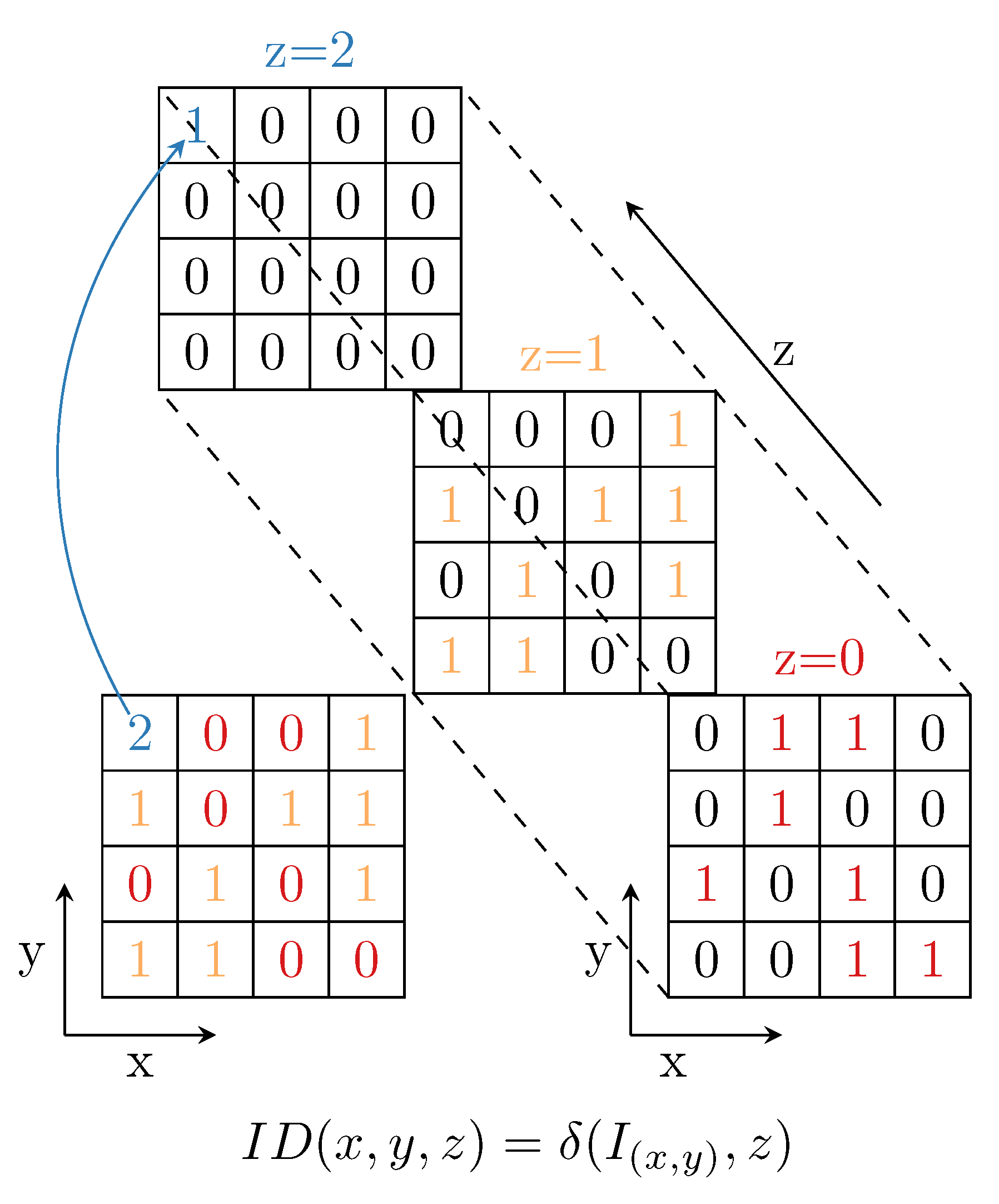
3.1. Indicator Array
First, the 2D image is transformed into a 3D indicator array, as depicted in Figure 1. The main steps are:
- create a 3D array putting a column over every pixel in the 2D image,
- the height of the column equals the number of discrete pixel value levels,
- the cells are filled with zeros, except the ones where the z coordinate of the cell equals the pixel value in the same (x,y) position in the image.
Using a Dirac function defined in Equation (9), the indicator array is as follows:
3.2. Weighted Contribution
The simplest weighting function is a constant value; this gives global ranking. A limited weighting function is often used having 1 as the weight for a small area around the selected pixel, and 0 elsewhere. This weighting function is called a ’window’, and the algorithm is a local histogram equalization. These histogram calculations can be implemented very efficiently. However, the most general form of weighting means evaluation of every pixel pair. If the image has n times n pixels, then the asymptotic complexity of this calculation is .
There is a special case when the weighting only depends on the distance of the pixel pairs.
In this special case, every pixel gives contribution at distance r.
Only pixels with this intensity value can contribute to a histogram bin . These pixels are recorded in the plane in the indicator array. Due to the translation invariant weights, the weighted histograms can be calculated convolving the indicator array in the plane z with the weighting function:
Convolutions can be efficiently calculated in the Fourier domain using fast Fourier transform (FFT), and its inverse (iFFT):
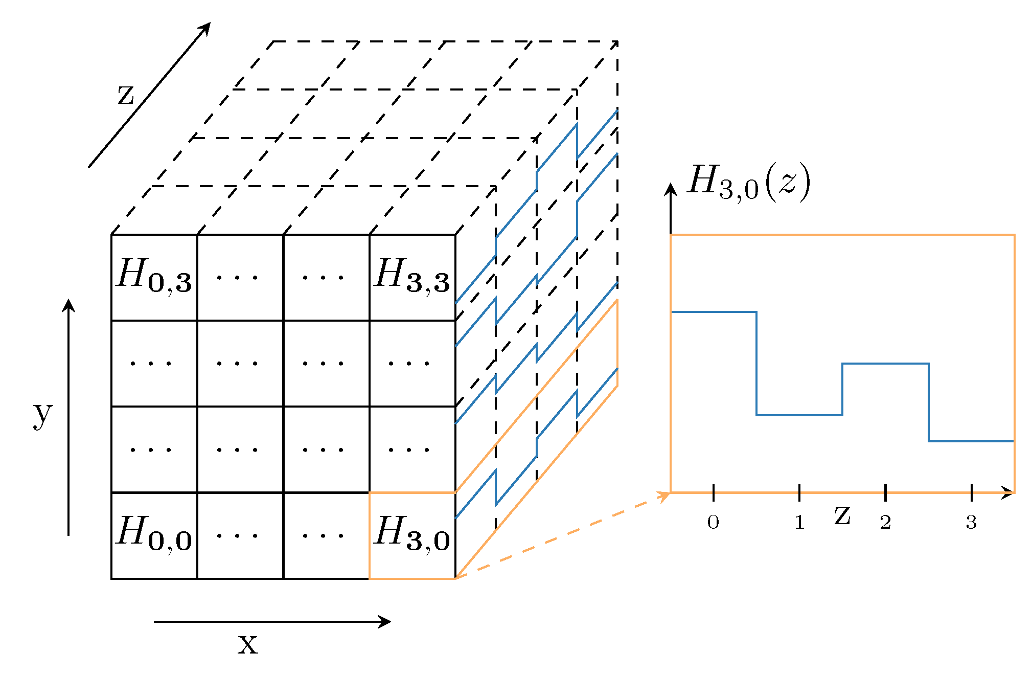
The result is a 3D array which contains locally weighted histograms along the z-direction for every corresponding pixel (see Figure 2). For further details, we refer the interested reader to [11].
Due to the nature of FFT, it is important to note that we used the ’mirrored image’ boundary condition, which is a frequently used condition for image boundaries when Fourier methods are used.
3.3. Relative Intensity
We define the relative intensity of a pixel in position based on the cumulative distribution function (CDF) of the local histograms:
This intensity should be converted to a pixel value using a perceptually linear color map.
3.4. Contrast Limit
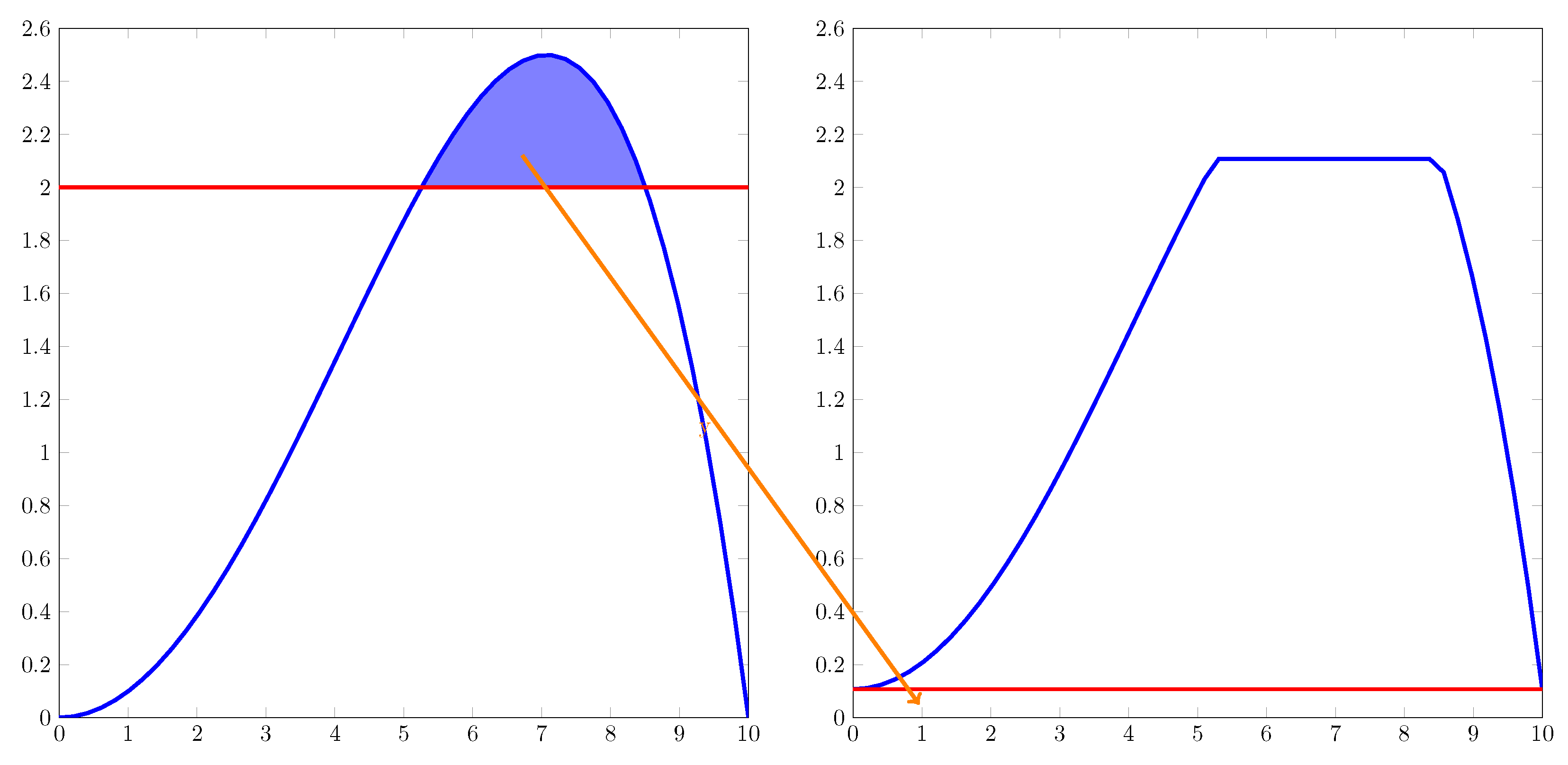
Contrast-limited adaptive histogram equalization (CLAHE) [7] introduced the idea of clipping histogram peaks and redistributing the clipped area to all histogram bins, as is depicted in Figure 3.
In our approach, a radially decreasing weight function yields good locality and avoids halos due to the large weighting kernel, but it still may over-stretch contrast between similar shades. Limiting contrast stretching effectively mitigates this issue, and avoids over-amplification of noise.
3.5. Algorithm Summary
The core algorithm can be summarized as follows:
- read data →,
- reduce bit depth with dithering →I,
- generate weight array,
- loop over pixel values (z),
- −
- ∗
- use superpixels, if downscaling is required,
- −
- convolve in x,y plane with W in order to get H,
- clip H peaks,
- redistribute clipped areas along the z-axis,
- determine local intensity from the local histogram and the original image
- −
- use bilinear interpolation, if superpixels were defined,
- convert the final result from float to integer with Floyd–Steinberg dithering.
4. Materials and Methods
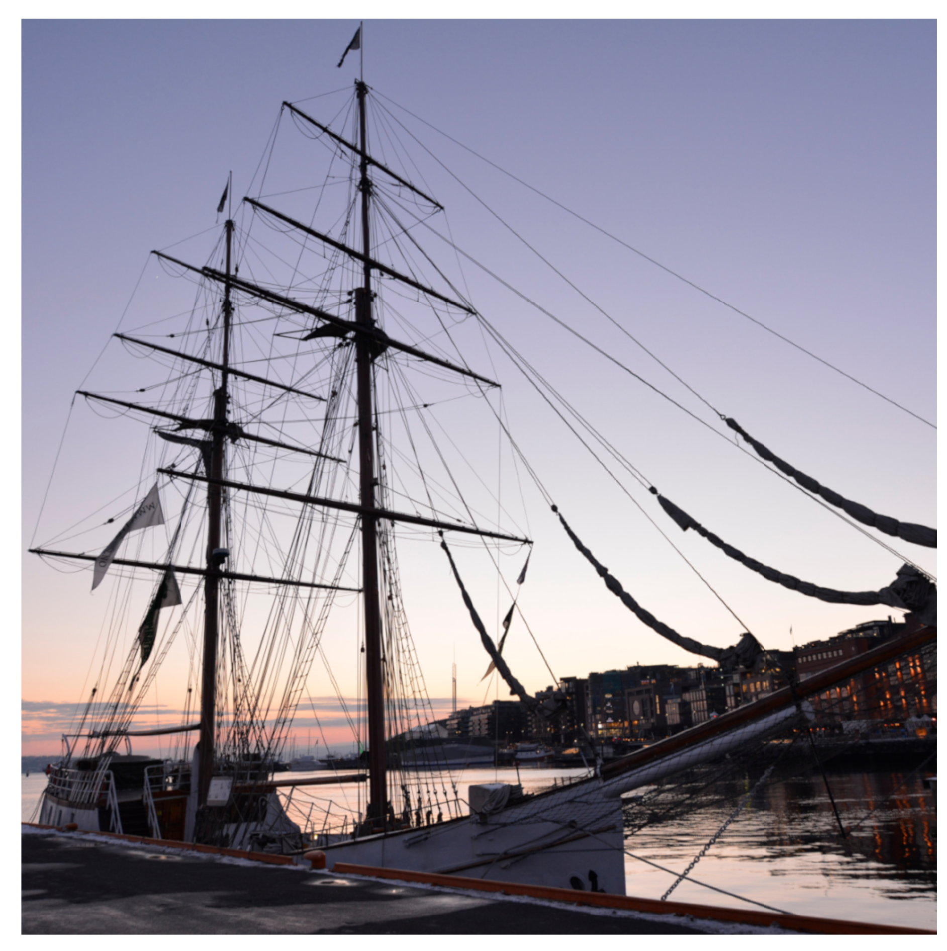
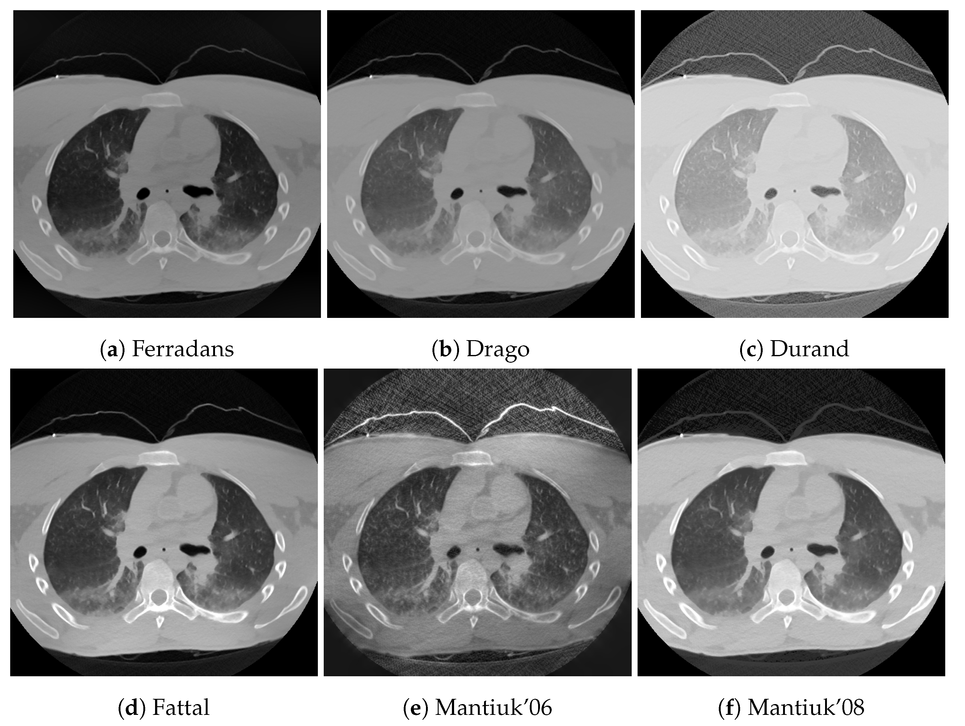
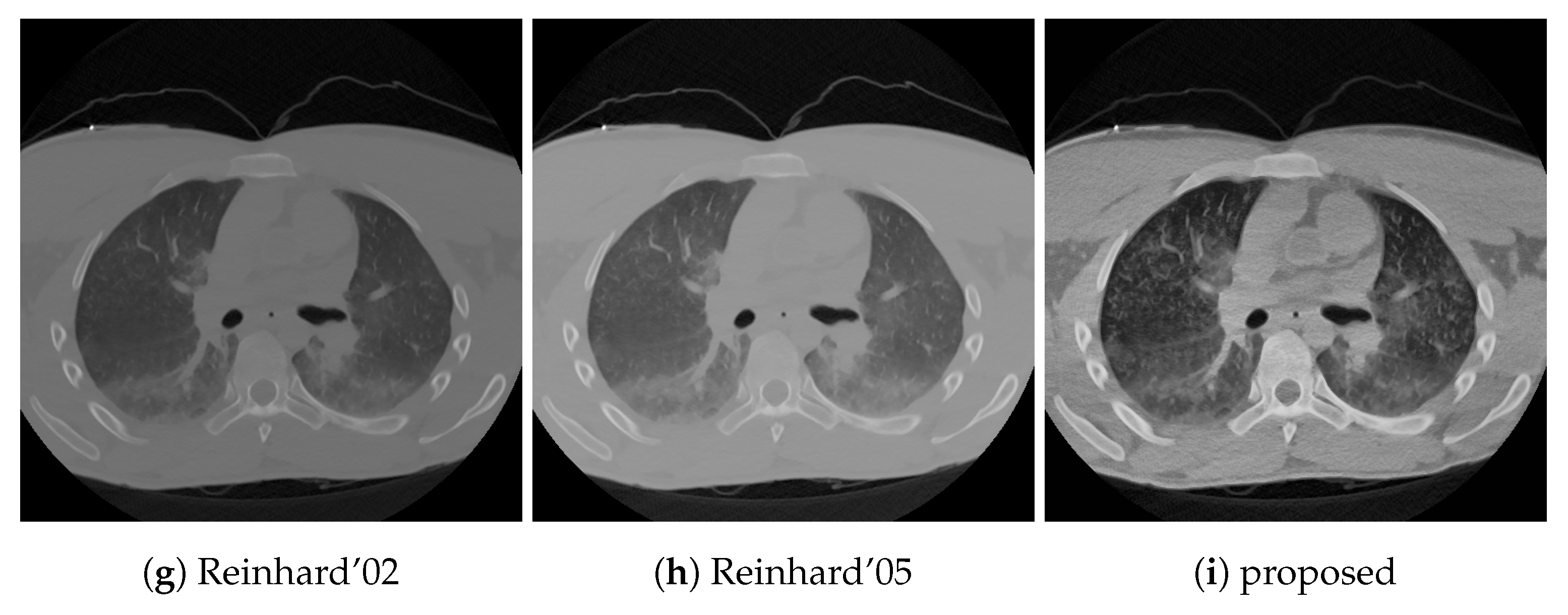
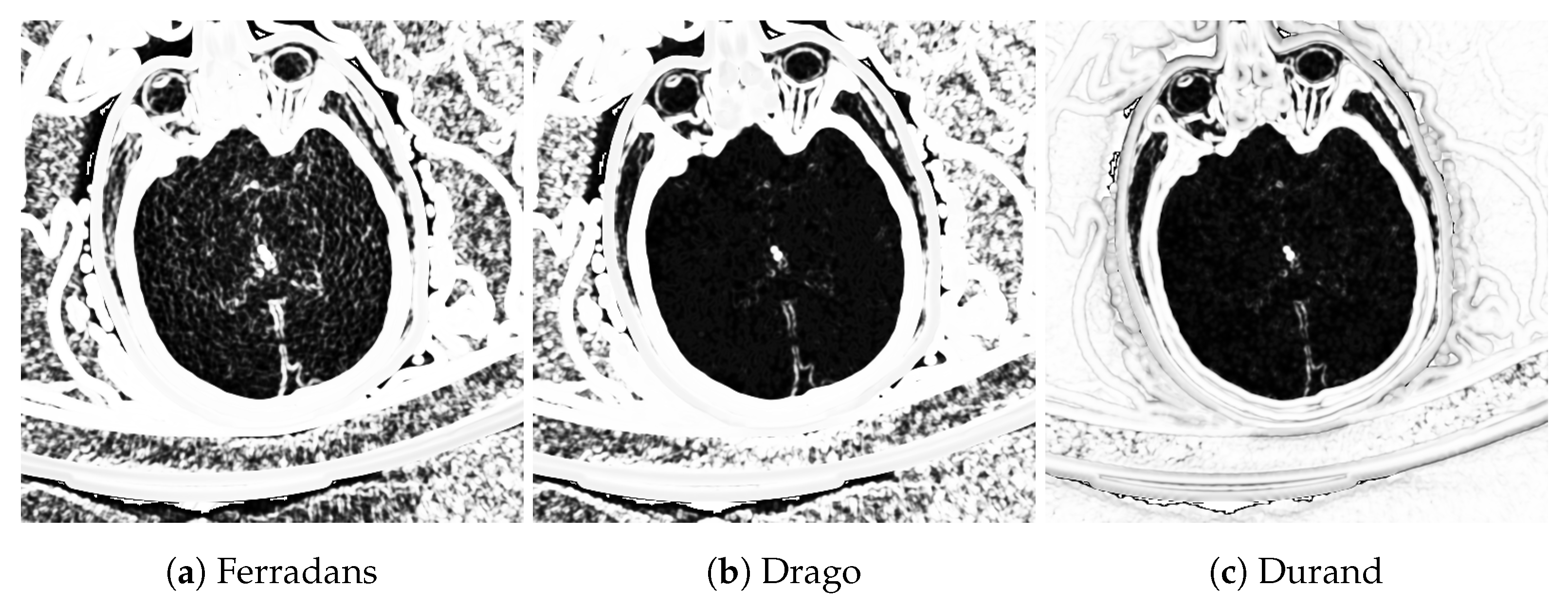
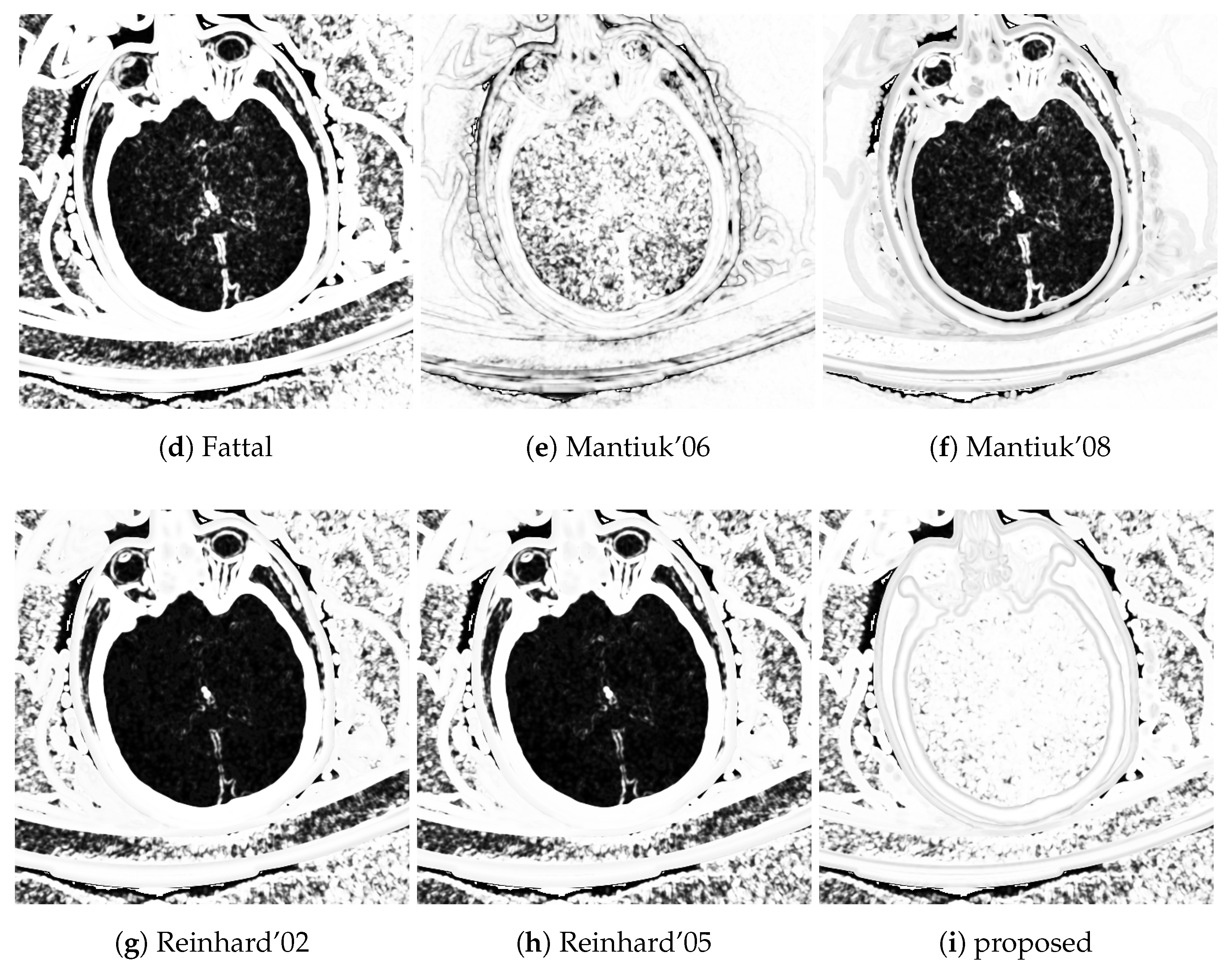
The results of our proposed algorithm are demonstrated in two ways. First, it has been compared to 8 different tone mapping operators, Ferradans [24], Drago [22], Durand [19], Fattal [21], Mantiuk ’06 [38] and ’08 [25], and Reinhard ’02 [20] and ’05 [23], using two post-mortem CT examples, a head and a chest CT. Second, the effects of changes of the algorithm parameters are depicted in two image montages, using the above-mentioned chest CT and a color photo of a ship, in Figure 4. The purpose of the ship image is to demonstrate that the algorithm is not specific to CT images. The image is an RGB image which was transformed to HSV color space [9], and the V component was processed using 256 discretization levels.
The presented CT examples are anonymized post mortem forensic CT images. The data collection was performed by the Oslo University Hospital, Department of Forensic Sciences, and was approved by the Attorney General of Norway. Next of kin were informed of the right to opt out from use of data in research projects. The ship photo was taken by the first author.
The CT image uses Hounsfield units; the pixel value range was −1024, +3069 HU for the chest, and −1024, +1935 HU for the head CT scan, using 1 HU step. The resolution of the ship image is 1024 × 1024 pixels, while the CT images natively have 512 × 512 pixel resolution.
4.1. Evaluation
Three evaluation metrics are used to present our results: the structural part of the tone mapped image quality index (TMQI) [39], image entropy, and gradient magnitude. TMQI is a metric for determining image quality of tone mapped images using a high dynamic range original as a reference image. It correlates the pixels of the original image and the tone mapped image using Pearson correlation. The correlation is calculated at five different scales, and weighted combination of the coefficients gives the structural similarity component of the TMQI score. The score should be between and 1, and the higher value indicates better structural match. Entropy and gradient magnitude are used as image descriptors. Entropy measures how well the dynamic range is utilized. It gives a high value when the levels in the dynamic range are uniformly utilized. While entropy measures a global property of the image, gradient magnitude measures a local one. Gradient magnitude measures the averaged amount of edges in an image. A higher value indicates more or larger edges, which indicates more details in the image. Neither entropy nor gradient magnitude determine perceived image quality, as they do not take the human visual system into account; however, as a frequently used image, they can contribute to the characterization of the proposed algorithm.
These descriptors above are used to compare the tone mapping operators to the proposed algorithm in two cases: a chest CT where the low tissue densities (lungs) are significant, and a head CT where the medium densities (white and gray matter) play an important role.
The parameters for the algorithms are presented in Table 1. They were selected using a grid-search algorithm around the recommended parameter settings. The parameter combination was selected which yielded the highest combined TMQI score for the two CT images. The proposed algorithm has a relatively wide parameter range where the TMQI score is stable. From this range, , were selected, as convenient integer parameters.
4.2. Implementation
Our algorithm is implemented in Python3.6 [40] using Numpy 1.13.3 [41], Scipy 1.0.1 [42], and Numba 0.38.0 [43]. For color space transformation, scikits-image 0.14.0 [44] was used. The source code follows PEP8 [45] recommendations and is part of the supplementary material. Luminance HDR 2.5.1 [46] was used to generate the reference TMO images, using the Ubuntu 18.04 operating system. The TMQI score is calculated using the original source code from the authors [39], using Octave 4.2.2 [47]. All of the custom calculation codes, as well as the example images, are available as a supplement to the paper.
The calculations were performed on a Dell Latitutde E7440 notebook (Round Rock, TX, USA) which was equipped with an Intel(R) Core(TM) i7-4600U CPU @ 2.10GHz (Santa Clara, CA, USA), 8GB of DDR3 RAM at 1600MT/s transfer speed. The data was stored on a 240 GB SAMSUNG SSD PM85 drive (San Jose, CA, USA), using btrfs filesystem. The operating system was Ubuntu 18.04 64bit. The computation time is dominated by the FFT calculation for which we used the Scipy implementation, but this part could be replaced with other numerical libraries, or could be executed on GPUs. However, some constant overhead is inevitable due to disk reading, data conversion, initializations, etc.
5. Discussion
The main difference between the proposed algorithm and traditional histogram equalization methods is the power-law-based distance-weighted contribution to the local histograms. LHE and CLAHE are special cases in our proposed generalized framework with constant spatial weights with radial cut-off (CLAHE) or without it (HE). While a similar approach is used for other types of weighting functions, we are not aware of power-law-based weighting. However, power-law was proposed as part of a generalized cumulation function-based histogram equalization [14]. This method is orthogonal to our approach because the Fourier series-based convolution approach is used on the intensity axis of the 3D histogram, while our method uses convolution along the spatial axes.
Many novel histogram-based methods try to modify or prescribe the shape of the local histograms but leave the spatial part intact. These methods, for instance, the bi-histogram equalization, could be easily combined with our approach, and therefore, we see these algorithms as complementers.
Traditional TMOs offer dynamic range compression with low noise but good local contrast. These operators perform well for selected sub-problems, usually either for low densities (lung) or for high densities (bones). The challenge for these algorithms is to reproduce good local contrast for medium densities (soft tissues) where the contrast is already low in the source. This situation is common in head CTs where the soft tissue contrast is poor.
As can be seen in Table 2, the proposed algorithm yields good structural similarity scores. The structural similarity score is from the TMQI algorithm’s structural similarity part. TMQI was developed for natural images, and it contains a ’naturalness’ component. This does not seem applicable to medical images, and we only present the structural score. However, if naturalness was taken into account, it would not change the conclusions.
A shortcoming of all of the scores, not only TMQI, is that they do not take into account the image content. Photographic images usually use the whole pixel domain to present information. In CT scans, information from outside of the human body has a limited role, and pixels outside of the scan field of view do not contribute to the image quality, but they are present in the DICOM files as zero pixels. Neither TMQI score nor the tone mapping algorithms take this into account.
Structural similarity is not equally important in all parts of CT scans. It can be argued that a content-aware structural similarity metric should be developed in the future which takes the field-of-view and tissue properties into account. We are not aware of such a content-dependent performance metric for CT images, and it is beyond the scope of this paper to introduce one, but we recognize this limitation.
TMQI offers structural similarity maps at various resolution levels. Figure 9 shows the finest resolution structural similarity maps of the different tone mapping operators using the head CT example. The advantage of the proposed method is that it has better structural similarity for medium densities, e.g., white and gray matter in the brain, than the alternative methods which mostly perform well outside of the skull.
5.1. Distance Metric
Equation (12) uses a Euclidian distance metric. Other distance metrics could be also used, e.g., Manhattan or maximum distances. Choosing a different distance did not visibly change the example images, but an image with a lot of directed structures might be sensitive to the distance metric selection. We always recommend the Euclidian metric because it is rotationally invariant.
The metric has to be invariant to translation, otherwise FFT could not be utilized for an efficient convolution calculation. While a position-dependent metric could be interesting, it would yield a much less efficient calculation scheme than the FFT-based convolution.
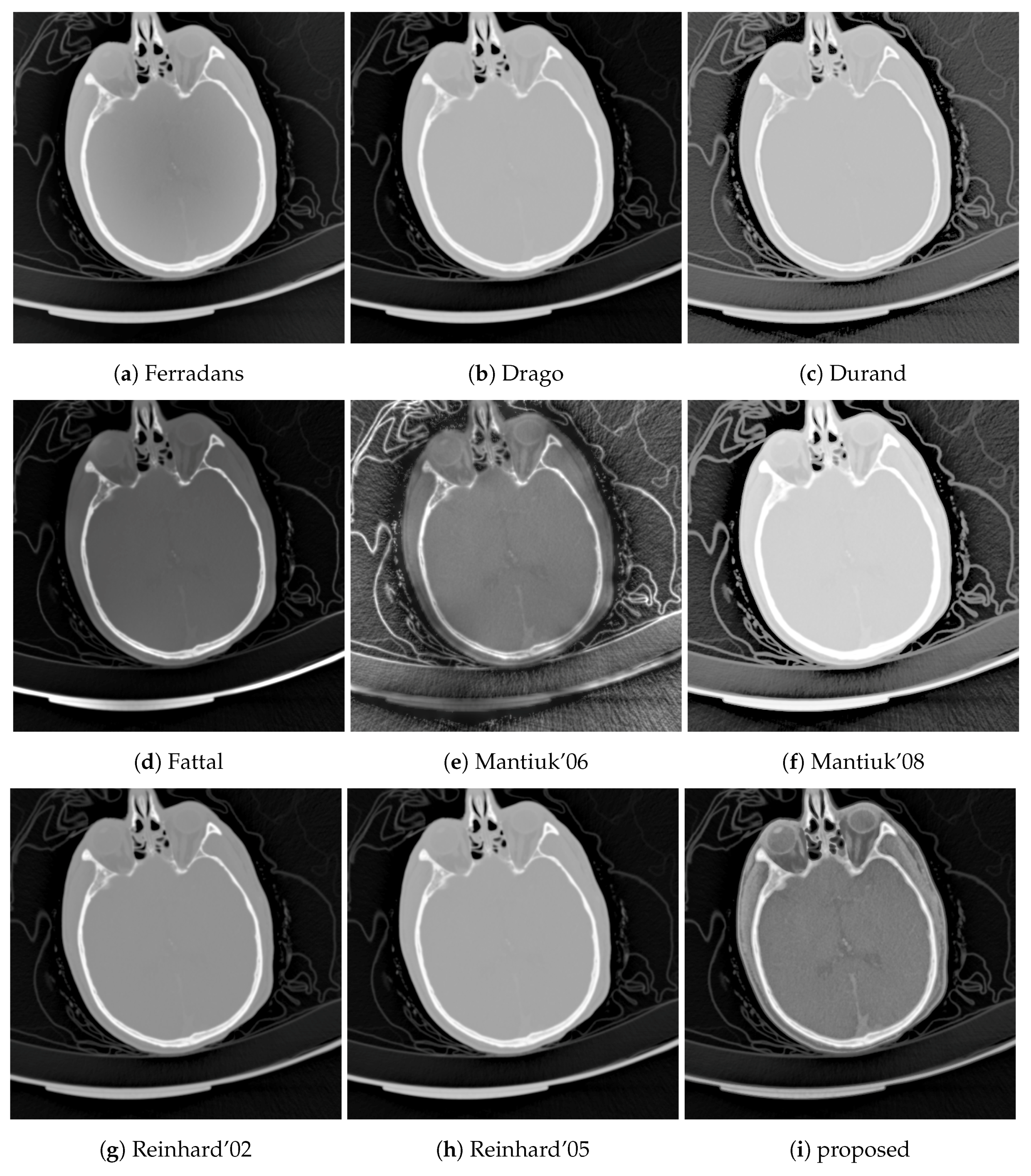
5.2. Locality and Clipping Limits
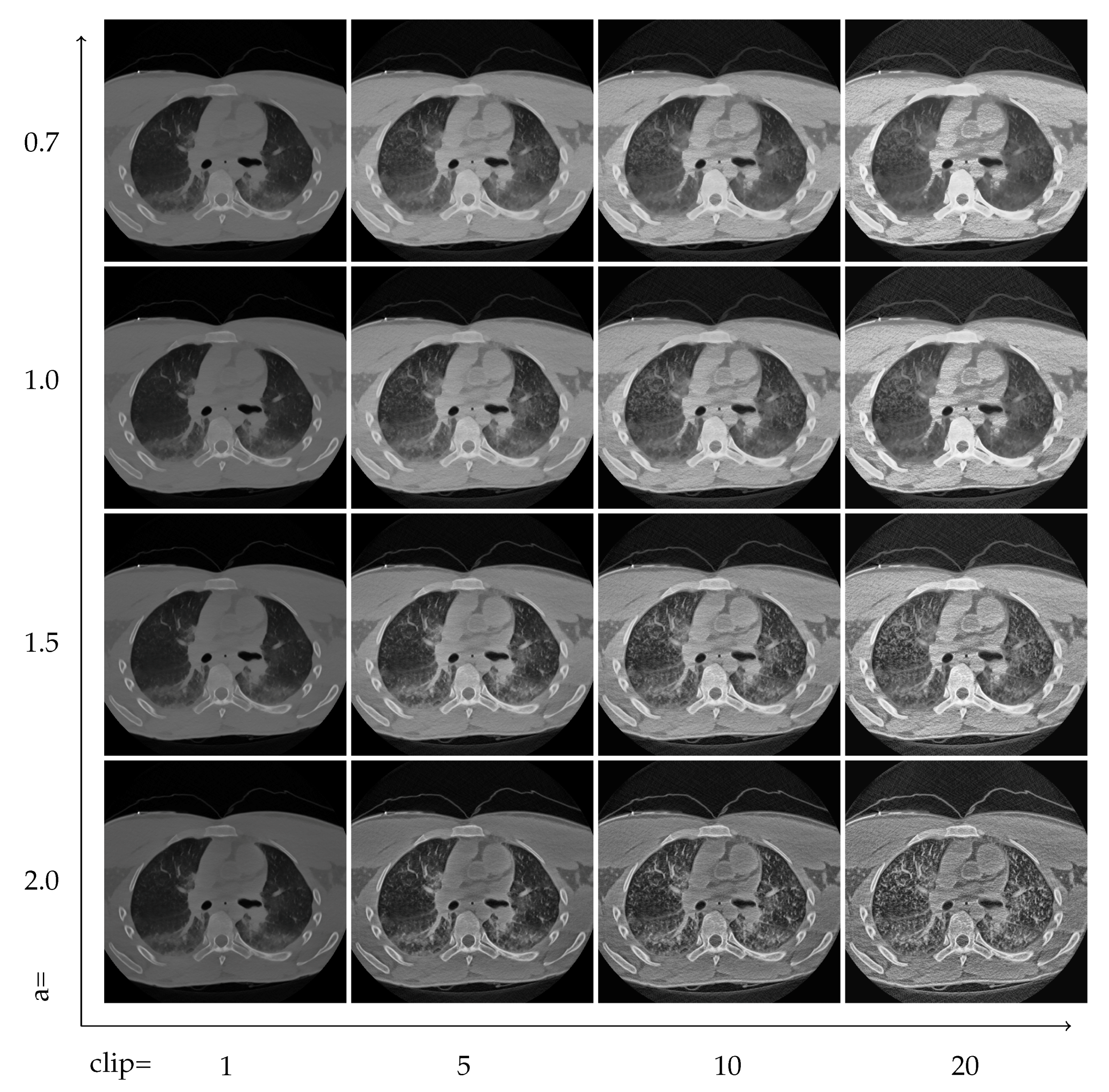
The two control parameters strongly affect the quality of the resulting images. However, finding the right balance can strongly depend on the visualization goal. Higher exponents mean stronger local contrast enhancement, but can also enhance noise. The contrast limit works against the distortions, but also limits the achievable feature amplification. Two image grids in Figure 7 and Figure 8 demonstrate these issues.
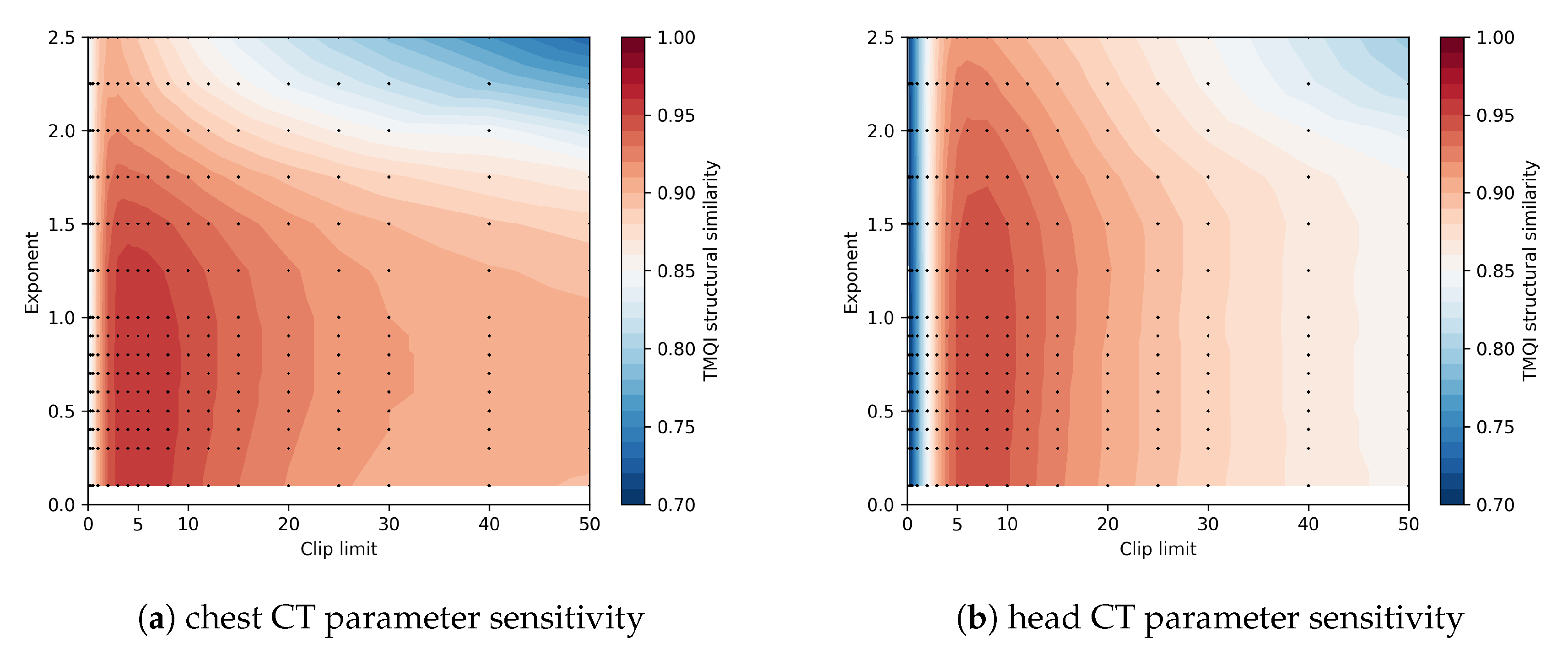
The parameter sensitivity of the algorithm is an important question. The TMQI structural similarity score is depicted in Figure 10 as the function of the exponent and the clip limit. There is a central region where the TMQI score is relatively stable and any parameter pair from this range is a reasonably good choice, e.g., , seems to be a good starting point. As will be discussed in the Optimization section, the calculation can be sped up without sacrificing the image quality too much. With lower precision calculations, the parameter space is quickly discoverable.
5.3. Edge Enhancement and Auto-Leveling
As was mentioned in Equation (7), base-detail layer separation is a frequent approach. Edges could be separated from the image, and added back to the compressed image. However, this technique is applicable to all tone mapping approaches. Such edge enhancement was not applied for the reference operators, and, for the sake of fair comparison, the proposed method does not contain such edge enhancement either. Similarly, auto-leveling, a method which slightly stretches image contrast, was not applied in the traditional TMOs or in our proposed method.
5.4. Asymptotic Complexity
Asymptotic complexity is dominated by the calculation of the weighted histogram array. Calculating weights directly between pixel pairs has a complexity of .
Creating the indicator array is proportional to the number of pixels: . Fast Fourier Transform of a array requires two one-dimensional FFTs for every line (n), and the cost of one line’s transform is . The number of 2D arrays is proportional to the number of different pixel-value levels (m). Taking all of these into account, the asymptotic complexity is:
As long as , this is a faster approach than weights taken directly from pixel pairs. This condition is easily met for traditional photographs which usually have pixels for image width and height while the number of discrete levels is usually between 256 and 1024. In some medical applications, the image resolution is lower, while the number of levels is higher. For instance, computed tomography usually has images with 512 × 512 pixels with 4096 different quantization levels.
Color images are usually processed in an 8- or 10-bit discretized brightness, lightness or value channel, but conversion from another color space with a large dynamic range might yield a huge number of levels, e.g., directly processing RAW data from digital cameras. A huge number of discrete levels might render the approach non-beneficial, or would require approximations, as is explained later in Section 6.
5.5. Memory Consumption
Similar to the notation, we use for space complexity.
Convolution-based calculation produces the whole histogram array at once before it could be used for further calculation. This means space complexity.
However, local histograms could be calculated directly using the pairwise weight calculation. This approach only needs to store one local histogram () the input image and the output image ().
This means that there is a trade-off between space complexity and time complexity. The convolution-based algorithm has better asymptotic time complexity but an order of magnitude worse space complexity than the direct pairwise method.
6. Optimization
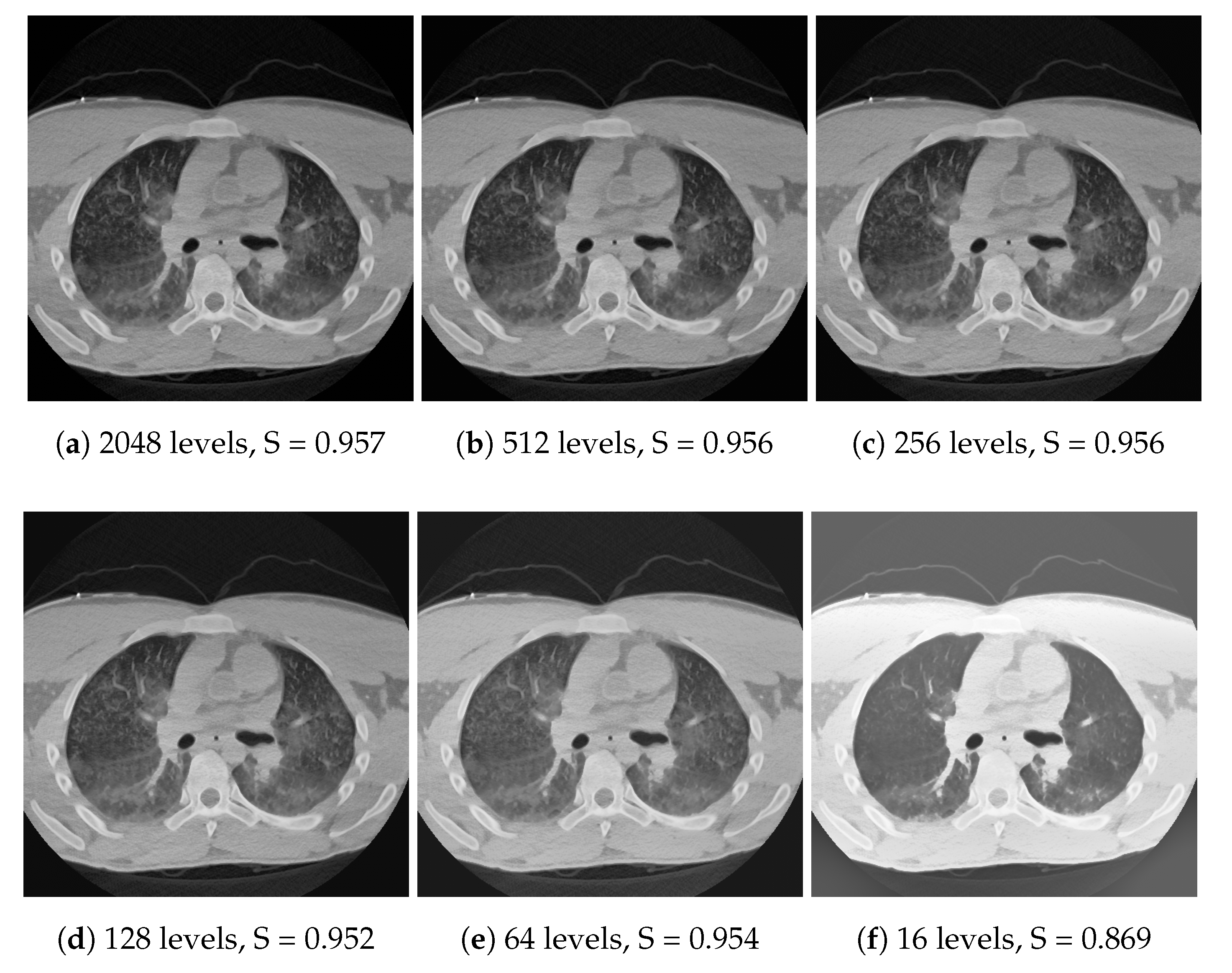
There are two easy ways to optimize performance. First, the number of shades can be effectively reduced. Locally, the only factor taken into account for a single pixel is the weighted number of pixels which have lower or higher values than the current given pixel. The number of shades could be reduced significantly without a noticeable difference in the output, if the values are binned with error diffusion, also known as dithering. When the local histograms are ready, the final intensities should be calculated using linear interpolation between the discretization levels. Usual histogram processing methods are not sensitive to a large amount of gray levels, and this dithered downsampling of the histogram has not been used before, to the best of our knowledge. Dithering is also used after the tone mapping in order to decorrelate the discretization error. Both dithering steps use the Floyd–Steinberg algorithm [48].
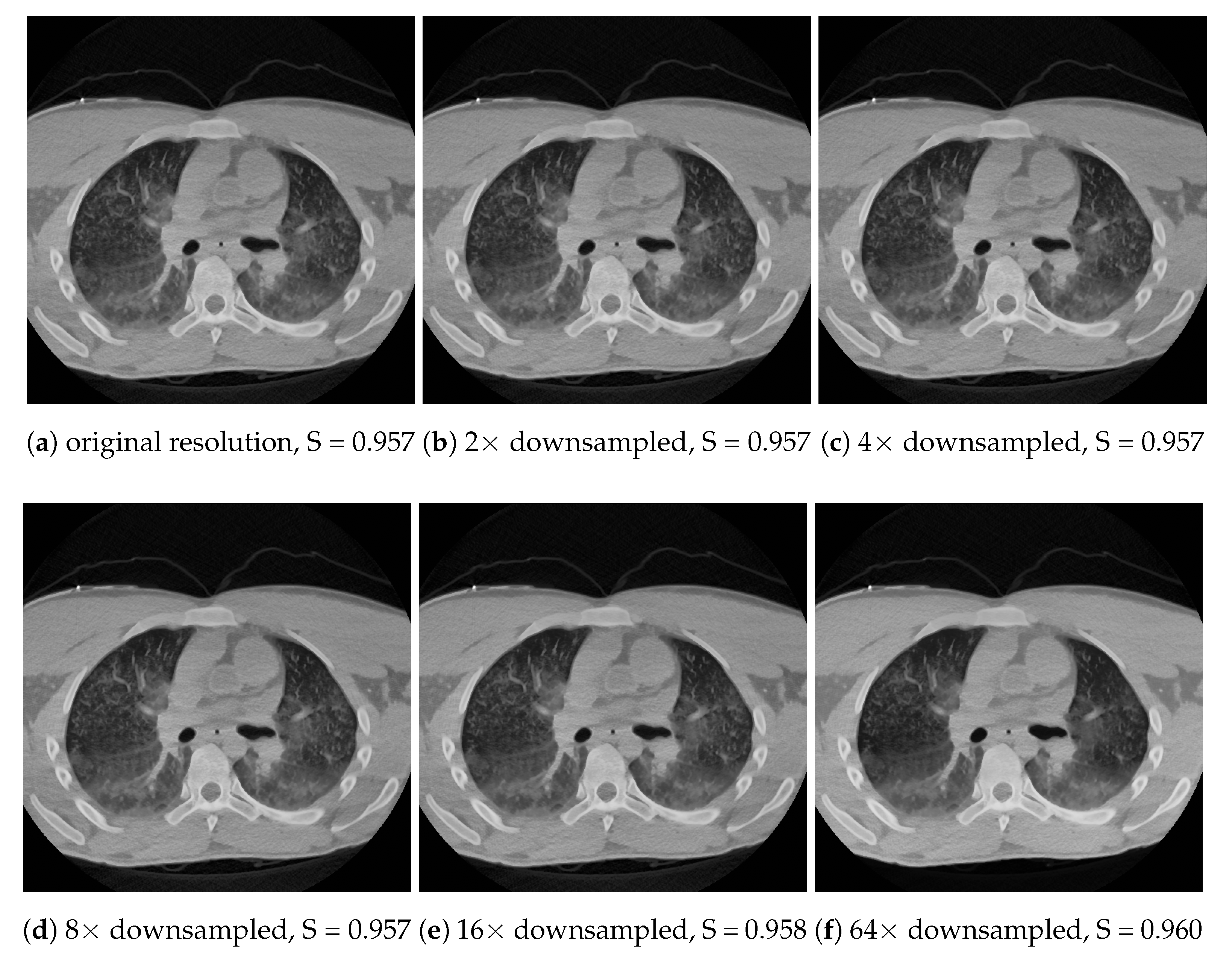
Another optimization possibility is to downsample the image during the histogram calculation, and perform the tone mapping using the downsampled histogram. Technically, this means a histogram column gets a contribution from several image pixels. No pixel data is lost during this downsampling, but the spatial resolution of the histogram array is decreased. This interpolation technique is mentioned in [11]. These histograms can be bilinearly interpolated for any interior point when it is required for the tone mapping.
Both spatial downsampling and dithering build on the fact that important features in the images usually have a larger area than a few pixels, and the local histograms do not change too fast; therefore, the 3D histogram can be approximated well with one which has reduced resolution along all axes. As long as these assumptions are valid, the tone mapping can approximately linearly speed up with downsampling in terms of the number of pixels and/or shades. Memory consumption scales down in a similar manner. The effect of the techniques can be seen in Figure 11 and Figure 12 for dithering and downscaling, respectively. Note that the downscaling is meant for each axis. For instance, a 64× downsample means only eight samples along each axis, and 64 samples in total for a CT image with 512 × 512 pixels.
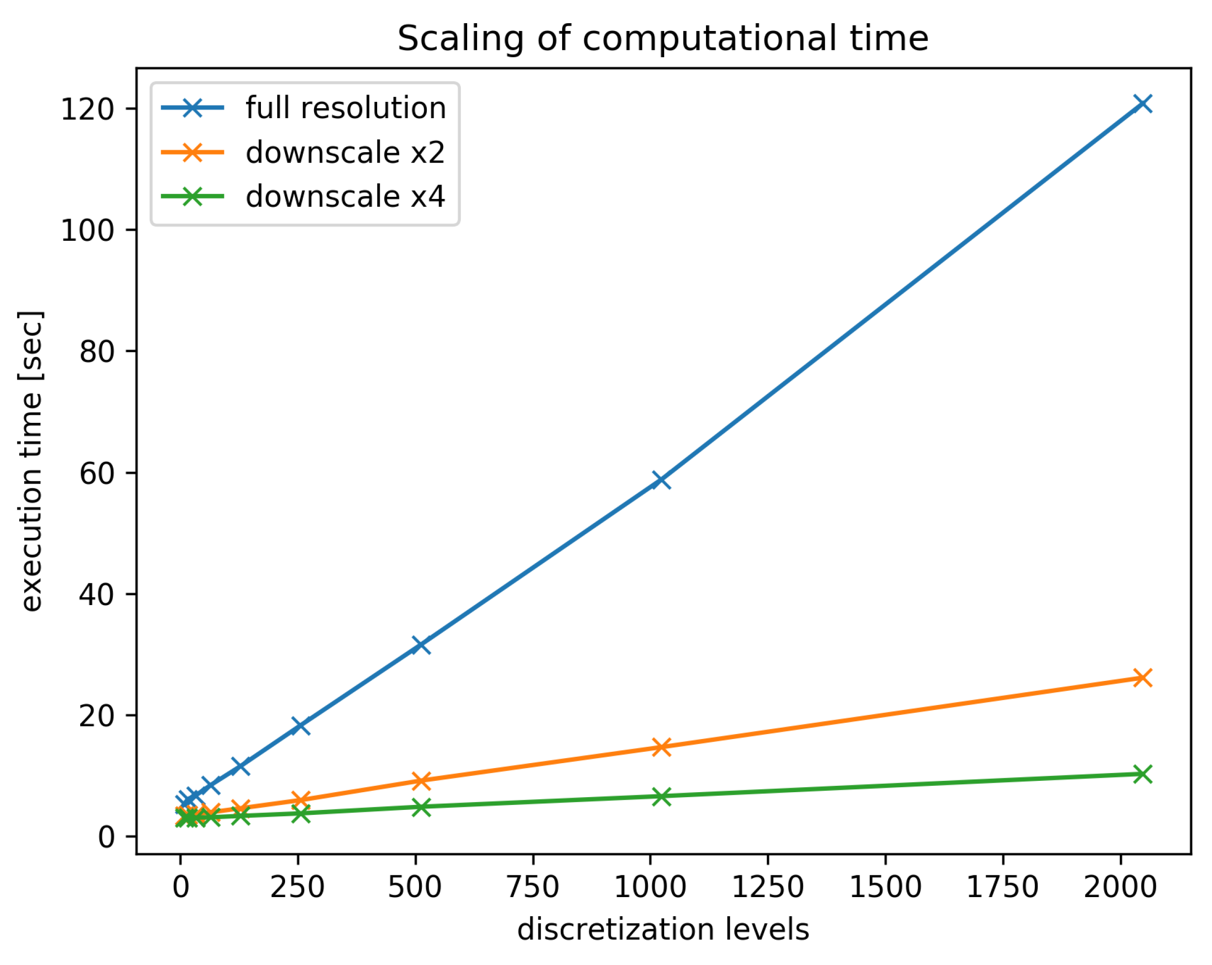
In both cases, the linear interpolation makes the approximation robust, which to a certain extent can compensate for the downsampling error, both in spatial and in color space. In exchange for precision loss, the computation time could be greatly reduced, as is shown in Figure 13. The execution time (t) is approximately linear in the number of pixels and in the discretizaton levels (D), not counting a small constant overhead (O). The number of pixels is inversely proportional to the square of the downscaling factor(x):
where c is a constant. The same result could be derived from Equation (18), with the constant approximation.
7. Conclusions
Our proposed method yields good local contrast for CT images while maintaining a similar image structure to the reference CT image. This could contribute to improving the visualization of pathologies. The proposed method performs well in terms of structural similarity compared to popular tone mapping algorithms. The computation cost can be effectively reduced with approximations.
Supplementary Materials
The following are available at https://www.mdpi.com/1999-4893/11/8/111/s1, algorithm source code.
Author Contributions
Methodology, D.V.; Software, D.V.; Supervision, A.C.T.M., A.S.-P., D.W. and M.P.; Visualization, D.V.; Writing—Original draft, D.V.; Writing—Review & editing, D.V., A.C.T.M., A.S.-P., D.W. and M.P.
Funding
This research was been funded by the Research Council of Norway through project no. 221073 ‘HyPerCept—Colour and quality in higher dimensions’.
Conflicts of Interest
The authors declare no conflict of interest.
References
- Barrett, J.F.; Keat, N. Artifacts in CT: recognition and avoidance. RadioGraphics 2004, 24, 1679–1691. [Google Scholar] [CrossRef] [PubMed]
- John, A.; Huda, W.; Scalzetti, E.M.; Ogden, K.M.; Roskopf, M.L. Performance of a single lookup table (LUT) for displaying chest CT images1. Acad. Radiol. 2004, 11, 609–616. [Google Scholar] [CrossRef] [PubMed]
- Fayad, L.M.; Jin, Y.; Laine, A.F.; Berkmen, Y.M.; Pearson, G.D.; Freedman, B.; Van Heertum, R. Chest CT window settings with multiscale adaptive histogram equalization: Pilot study. Radiology 2002, 223, 845–852. [Google Scholar] [CrossRef] [PubMed]
- Chang, A.E.; Matory, Y.L.; Dwyer, A.J.; Hill, S.C.; Girton, M.E.; Steinberg, S.M.; Knop, R.H.; Frank, J.A.; Hyams, D.; Doppman, J.L. Magnetic resonance imaging versus computed tomography in the evaluation of soft tissue tumors of the extremities. Ann. Surg. 1987, 205, 340–348. [Google Scholar] [CrossRef] [PubMed]
- Seeram, E. Computed Tomography-E-Book: Physical Principles, Clinical Applications, and Quality Control; Elsevier Health Sciences: St. Louis, Missouri, USA, 2015. [Google Scholar]
- Lehr, J.L.; Capek, P. Histogram equalization of CT images. Radiology 1985, 154, 163–169. [Google Scholar] [CrossRef] [PubMed]
- Zuiderveld, K. Graphics Gems IV; Chapter Contrast Limited Adaptive Histogram Equalization; Academic Press Professional, Inc.: San Diego, CA, USA, 1994; pp. 474–485. [Google Scholar]
- Cohen-Duwek, H.; Spitzer, H.; Weitzen, R.; Apter, S. A biologically-based algorithm for companding computerized tomography (CT) images. Comput. Biol. Med. 2011, 41, 367–379. [Google Scholar] [CrossRef] [PubMed]
- Acharya, T.; Ray, A.K. Image Processing: Principles and Applications; John Wiley & Sons: Hoboken, NJ, USA, 2005. [Google Scholar]
- Nikvand, N.; Yeganeh, H.; Wang, Z. Adaptive windowing for optimal visualization of medical images based on normalized information distance. In Proceedings of the 2014 IEEE International Conference on Acoustics, Speech and Signal Processing (ICASSP), Florence, Italy, 4–9 May 2014. [Google Scholar] [CrossRef]
- Pizer, S.M.; Amburn, E.P.; Austin, J.D.; Cromartie, R.; Geselowitz, A.; Greer, T.; ter Haar Romeny, B.; Zimmerman, J.B.; Zuiderveld, K. Adaptive histogram equalization and its variations. Comput. Vis. Gr. Image Process. 1987, 39, 355–368. [Google Scholar] [CrossRef]
- Kim, Y.T. Contrast enhancement using brightness preserving bi-histogram equalization. IEEE Trans. Consum. Electron. 1997, 43, 1–8. [Google Scholar] [CrossRef]
- Nikolova, M.; Wen, Y.W.; Chan, R. Exact Histogram Specification for Digital Images Using a Variational Approach. J. Math. Imaging Vis. 2012, 46, 309–325. [Google Scholar] [CrossRef] [Green Version]
- Stark, J. Adaptive image contrast enhancement using generalizations of histogram equalization. IEEE Trans. Image Process. 2000, 9, 889–896. [Google Scholar] [CrossRef] [PubMed] [Green Version]
- Pattanaik, S.N.; Ferwerda, J.A.; Fairchild, M.D.; Greenberg, D.P. A multiscale model of adaptation and spatial vision for realistic image display. In Proceedings of the 25th Annual Conference on Computer Graphics and Interactive Techniques—SIGGRAPH ’98, Orlando, FL, USA, 19–24 July 1998; ACM Press: New York, NY, USA, 1998. [Google Scholar]
- Farbman, Z.; Fattal, R.; Lischinski, D.; Szeliski, R. Edge-preserving decompositions for multi-scale tone and detail manipulation. In ACM SIGGRAPH 2008 Papers on—SIGGRAPH ’08; ACM Press: New York, NY, USA, 2008. [Google Scholar]
- Zhang, Z.; Su, Z. Tone mapping via edge-preserving total variation model. In Proceedings of the 2012 5th International Congress on Image and Signal Processing, Chongqing, China, 16–18 October 2012. [Google Scholar] [CrossRef]
- Tan, L.; Liu, X.; Xue, K. A Retinex-Based Local Tone Mapping Algorithm Using L 0 Smoothing Filter. In Communications in Computer and Information Science; Springer: Berlin, Germany, 2014; pp. 40–47. [Google Scholar]
- Durand, F.; Dorsey, J. Fast bilateral filtering for the display of high-dynamic-range images. ACM Trans. Gr. 2002, 21. [Google Scholar] [CrossRef] [Green Version]
- Reinhard, E.; Stark, M.; Shirley, P.; Ferwerda, J. Photographic tone reproduction for digital images. In Proceedings of the 29th Annual Conference on Computer Graphics and Interactive Techniques—SIGGRAPH ’02, San Antonio, TX, USA, 21–26 July 2002; ACM Press: New York, NY, USA, 2002. [Google Scholar]
- Fattal, R.; Lischinski, D.; Werman, M. Gradient domain high dynamic range compression. In Proceedings of the 29th Annual Conference on Computer Graphics and Interactive Techniques—SIGGRAPH ’02, San Antonio, TX, USA, 21–26 July 2002; ACM Press: New York, NY, USA, 2002. [Google Scholar] [CrossRef]
- Drago, F.; Myszkowski, K.; Annen, T.; Chiba, N. Adaptive Logarithmic Mapping For Displaying High Contrast Scenes. Comput. Gr. Forum 2003, 22, 419–426. [Google Scholar] [CrossRef] [Green Version]
- Reinhard, E.; Devlin, K. Dynamic range reduction inspired by photoreceptor physiology. IEEE Trans. Vis. Comput. Gr. 2005, 11, 13–24. [Google Scholar] [CrossRef] [PubMed]
- Ferradans, S.; Bertalmio, M.; Provenzi, E.; Caselles, V. An Analysis of Visual Adaptation and Contrast Perception for Tone Mapping. IEEE Trans. Pattern Anal. Mach. Intell. 2011, 33, 2002–2012. [Google Scholar] [CrossRef] [PubMed] [Green Version]
- Mantiuk, R.; Daly, S.; Kerofsky, L. Display adaptive tone mapping. In ACM SIGGRAPH 2008 Papers on—SIGGRAPH ’08; ACM Press: New York, NY, USA, 2008. [Google Scholar]
- Meylan, L.; Susstrunk, S. High dynamic range image rendering with a retinex-based adaptive filter. IEEE Trans. Image Process. 2006, 15, 2820–2830. [Google Scholar] [CrossRef] [PubMed] [Green Version]
- Fairchild, M.D.; Johnson, G.M. Meet iCAM: A next-generation color appearance model. In Color and Imaging Conference; Society for Imaging Science and Technology: Springfield, VA, USA, 2002; Number 1; pp. 33–38. [Google Scholar]
- Reinhard, E.; Heidrich, W.; Debevec, P.; Pattanaik, S.; Ward, G.; Myszkowski, K. High Dynamic Range Imaging; Morgan Kaufman: San Francisco, CA, USA, 2006. [Google Scholar]
- Mantiuk, R.K.; Karol, M.; Hans-Peter, S. High Dynamic Range Imaging. In Wiley Encyclopedia of Electrical and Electronics Engineering; John Wiley & Sons, Inc.: Hoboken, NJ, USA, 2015; pp. 1–42. [Google Scholar]
- Banterle, F.; Artusi, A.; Debattista, K.; Chalmers, A. Advanced High Dynamic Range Imaging: Theory and Practice, 2nd ed.; AK Peters (CRC Press): Natick, MA, USA, 2017. [Google Scholar]
- Kalender, W.A. Computed Tomography: Fundamentals, System Technology, Image Quality, Applications; Publicis: Erlangen, Germany, 2011. [Google Scholar]
- Barrow, H.; Tenenbaum, J. Recovering intrinsic scene characteristics. Comput. Vis. Syst. 1978, 2, 3–26. [Google Scholar]
- Lepor, H. Prostatic Diseases; Number p. 966, v. 2000 in Prostatic Diseases; W.B. Saunders Company: Philadelphia, PA, USA, 2000. [Google Scholar]
- Gross, B.H.; Kazerooni, E.A. Cardiopulmonary Imaging; Lippincott Williams & Wilkins: Philadelphia, PA, USA, 2004. [Google Scholar]
- Wright, F.W. Radiology of the Chest and Related Conditions; Taylor & Francis: London, UK, 2001. [Google Scholar]
- Cooley, J.W.; Tukey, J.W. An algorithm for the machine calculation of complex Fourier series. Math. Comput. 1965, 19, 297. [Google Scholar] [CrossRef]
- Blommaert, F.J.; Martens, J.B. An object-oriented model for brightness perception. Spat. Vis. 1990, 5, 15–41. [Google Scholar] [CrossRef] [PubMed]
- Mantiuk, R.; Myszkowski, K.; Seidel, H.P. A perceptual framework for contrast processing of high dynamic range images. ACM Trans. Appl. Percep. 2006, 3, 286–308. [Google Scholar] [CrossRef] [Green Version]
- Yeganeh, H.; Wang, Z. Objective Quality Assessment of Tone-Mapped Images. IEEE Trans. Image Process. 2013, 22, 657–667. [Google Scholar] [CrossRef] [PubMed]
- Van Rossum, G.; Drake, F.L. Python 3 Reference Manual; CreateSpace: Paramount, CA, USA, 2009. [Google Scholar]
- Oliphant, T. Guide to NumPy; Continuum Press: Austin, TX, USA, 2015. [Google Scholar]
- Jones, E.; Oliphant, T.; Peterson, P. SciPy: Open Source Scientific Tools for Python. 2001. Available online: https://www.scipy.org (accessed on 12 June 2018).
- Lam, S.K.; Pitrou, A.; Seibert, S. Numba. In Proceedings of the Second Workshop on the LLVM Compiler Infrastructure in HPC—LLVM ’15, Austin, TX, USA, 15–20 November 2015; ACM Press: New York, NY, USA, 2015. [Google Scholar]
- Van der Walt, S.; Schönberger, J.L.; Nunez-Iglesias, J.; Boulogne, F.; Warner, J.D.; Yager, N.; Gouillart, E.; Yu, T. scikit-image: Image processing in Python. PeerJ 2014, 2, e453. [Google Scholar] [CrossRef] [PubMed]
- Van Rossum, G. PEP 8—Style Guide for Python Code. 2001. Available online: https://www.python.org/dev/peps/pep-0008 (accessed on 12 June 2018).
- Rota, G.; Comida, F.; Anastasia, D. Luminance HDR. 2006–2017. Available online: chttp://qtpfsgui.sourceforge.net (accessed on 12 June 2018).
- Eaton, J.W.; Bateman, D.; Hauberg, S.; Wehbring, R. GNU Octave Version 4.2.2 Manual: A High-Level Interactive Language for Numerical Computations. 2017. Available online: https://www.gnu.org/software/octave/doc/v4.2.2 (accessed on 12 June 2018).
- Floyd, R.W.; Steinberg, L. An Adaptive Algorithm for Spatial Greyscale. Proc. Soc. Inf. Disp. 1976, 17, 75–77. [Google Scholar]
Figure 1.
Indicator array generation: z coordinates are calculated from the pixel value of the 2D image.
Figure 1.
Indicator array generation: z coordinates are calculated from the pixel value of the 2D image.

Figure 2.
Columns in the z-direction contain the weighted histograms for corresponding pixels. Every pixel has its own local weighted histogram.
Figure 2.
Columns in the z-direction contain the weighted histograms for corresponding pixels. Every pixel has its own local weighted histogram.

Figure 3.
Local histograms might be clipped to reduce noise over-amplification.

Figure 4.
Harbour in sunset, taken by the first author. The fine details of the deck and the buildings are hidden in the shadow.
Figure 4.
Harbour in sunset, taken by the first author. The fine details of the deck and the buildings are hidden in the shadow.

Figure 5.
Tone mapped chest CT scan with eight common operators and the proposed method. Parameters are summarized in Table 1; a quantitative comparison is presented in Table 2.


Figure 6.
Tone mapped head CT scan with eight common operators and the proposed method. Parameters are summarized in Table 1; a quantitative comparison is presented in Table 2.

Figure 7.
The effect of the weighting function and clipping. Rows from top to bottom have a = 0.7, 1.0, 1.5, 2.0, respectively, and the clip limits in the columns from left to right are 1, 5, 10 and 20, using units where N is the number of histogram bins.
Figure 7.
The effect of the weighting function and clipping. Rows from top to bottom have a = 0.7, 1.0, 1.5, 2.0, respectively, and the clip limits in the columns from left to right are 1, 5, 10 and 20, using units where N is the number of histogram bins.

Figure 8.
The effect of the weighting function and clipping. Rows from top to bottom have a = 0.7, 1.0, 1.5, 2.0, respectively, and the clip limits in the columns from left to right are 1, 5, 10 and 20, using units where N is the number of histogram bins.
Figure 8.
The effect of the weighting function and clipping. Rows from top to bottom have a = 0.7, 1.0, 1.5, 2.0, respectively, and the clip limits in the columns from left to right are 1, 5, 10 and 20, using units where N is the number of histogram bins.

Figure 9.
Structural similarity map for the head CT example. Brighter shades belong to higher local structural similarity (white = 1.0, black = 0.0).
Figure 9.
Structural similarity map for the head CT example. Brighter shades belong to higher local structural similarity (white = 1.0, black = 0.0).


Figure 10.
Parameter sensitivity of the algorithm for (a) the chest CT, and (b) the head CT image.

Figure 11.
Calculating the histograms using a decreasing number of discretization levels. While quality slightly degrades after a while, the linear interpolation and dithering make the algorithm robust. TMQI structural similarity slowly decreases as the approximation becomes coarser.
Figure 11.
Calculating the histograms using a decreasing number of discretization levels. While quality slightly degrades after a while, the linear interpolation and dithering make the algorithm robust. TMQI structural similarity slowly decreases as the approximation becomes coarser.

Figure 12.
Calculating the histograms using spatial downsampling along each axis. Even significant downsampling does not cause very visible artefacts, which is also reflected in the TMQI score. However, local differences might appear, e.g., compare the middle region of the left lung in (a) and (f).
Figure 12.
Calculating the histograms using spatial downsampling along each axis. Even significant downsampling does not cause very visible artefacts, which is also reflected in the TMQI score. However, local differences might appear, e.g., compare the middle region of the left lung in (a) and (f).

Figure 13.
Approximate execution time scales with the number of pixels and the number of discretization levels plus a constant overhead because of data pre- and post-processing.
Figure 13.
Approximate execution time scales with the number of pixels and the number of discretization levels plus a constant overhead because of data pre- and post-processing.


Table 1.
Structural similarity scores from the TMQI algorithm, gradient magnitudes and image entropies. Bold text indicates the highest score.
Table 1.
Structural similarity scores from the TMQI algorithm, gradient magnitudes and image entropies. Bold text indicates the highest score.
| Algorithm | Chest CT | Head CT | Chest CT | Head CT | Chest CT | Head CT |
|---|---|---|---|---|---|---|
| TMQI | TMQI | grad.mag. | grad.mag. | Entropy | Entropy | |
| Drago | 0.904 | 0.794 | 0.208 | 0.202 | 5.96 | 5.85 |
| Durand | 0.899 | 0.749 | 0.212 | 0.207 | 6.12 | 6.18 |
| Fattal | 0.971 | 0.836 | 0.217 | 0.202 | 6.89 | 6.15 |
| Ferradans | 0.916 | 0.835 | 0.014 | 0.019 | 6.71 | 7.08 |
| Mantiuk’06 | 0.918 | 0.828 | 0.226 | 0.231 | 7.38 | 7.10 |
| Mantiuk’08 | 0.976 | 0.783 | 0.216 | 0.207 | 6.77 | 6.26 |
| Reinhard’02 | 0.898 | 0.803 | 0.206 | 0.202 | 5.81 | 5.86 |
| Reinhard’05 | 0.908 | 0.798 | 0.208 | 0.200 | 6.00 | 5.80 |
| proposed | 0.957 | 0.949 | 0.226 | 0.224 | 7.03 | 6.73 |
Table 2.
Parameter sets for the tone mapping operator.
| Algorithm | Parameters | |||
|---|---|---|---|---|
| Durand | = 7 | = 1.5 | base contrast = 4 | |
| Drago | bias = 1.0 | |||
| Fattal | alpha = 0.5 | beta = 0.95 | saturation = 1 | noise = 0.002 |
| Ferradans | rho = 0.4 | invAlpha = 5.5 | ||
| Mantiuk’06 | scaleFactor = 0.25 | saturationFactor = 0.5 | detailFactor = 7.0 | |
| Mantiuk’08 | saturation = 1 | contrast enhancement = 4.3 | ||
| Reinhard’02 | key = 0.02 | phi = 1.0 | no scales used | |
| Reinhard’05 | brightness = 7 | lightness adapt. = 1 | chromatic adapt. = 1 | |
| proposed | exponent = 1.0 | contrast limit = 6 | ||
© 2018 by the authors. Licensee MDPI, Basel, Switzerland. This article is an open access article distributed under the terms and conditions of the Creative Commons Attribution (CC BY) license (http://creativecommons.org/licenses/by/4.0/).
Share and Cite
MDPI and ACS Style
Völgyes, D.; Martinsen, A.C.T.; Stray-Pedersen, A.; Waaler, D.; Pedersen, M. A Weighted Histogram-Based Tone Mapping Algorithm for CT Images. Algorithms 2018, 11, 111. https://doi.org/10.3390/a11080111
AMA Style
Völgyes D, Martinsen ACT, Stray-Pedersen A, Waaler D, Pedersen M. A Weighted Histogram-Based Tone Mapping Algorithm for CT Images. Algorithms. 2018; 11(8):111. https://doi.org/10.3390/a11080111
Chicago/Turabian StyleVölgyes, David, Anne Catrine Trægde Martinsen, Arne Stray-Pedersen, Dag Waaler, and Marius Pedersen. 2018. "A Weighted Histogram-Based Tone Mapping Algorithm for CT Images" Algorithms 11, no. 8: 111. https://doi.org/10.3390/a11080111
Note that from the first issue of 2016, this journal uses article numbers instead of page numbers. See further details here.