A Novel Parallel Auto-Encoder Framework for Multi-Scale Data in Civil Structural Health Monitoring

1
School of Electrical Engineering, Computing and Mathematics Science, Curtin University, Kent Street, Bentley, WA 6102, Australia
2
Centre for Infrastructural Monitoring and Protection, School of Civil and Mechanical Engineering, Curtin University, Kent Street, Bentley, WA 6102, Australia
*
Author to whom correspondence should be addressed.
Algorithms 2018, 11(8), 112; https://doi.org/10.3390/a11080112
Submission received: 25 June 2018
/
Revised: 20 July 2018
/
Accepted: 24 July 2018
/
Published: 27 July 2018
(This article belongs to the Special Issue Discrete Algorithms and Discrete Problems in Machine Intelligence)
Abstract
:In this paper, damage detection/identification for a seven-storey steel structure is investigated via using the vibration signals and deep learning techniques. Vibration characteristics, such as natural frequencies and mode shapes are captured and utilized as input for a deep learning network while the output vector represents the structural damage associated with locations. The deep auto-encoder with sparsity constraint is used for effective feature extraction for different types of signals and another deep auto-encoder is used to learn the relationship of different signals for final regression. The existing SAF model in a recent research study for the same problem processed all signals in one serial auto-encoder model. That kind of models have the following difficulties: (1) the natural frequencies and mode shapes are in different magnitude scales and it is not logical to normalize them in the same scale in building the models with training samples; (2) some frequencies and mode shapes may not be related to each other and it is not fair to use them for dimension reduction together. To tackle the above-mentioned problems for the multi-scale dataset in SHM, a novel parallel auto-encoder framework (Para-AF) is proposed in this paper. It processes the frequency signals and mode shapes separately for feature selection via dimension reduction and then combine these features together in relationship learning for regression. Furthermore, we introduce sparsity constraint in model reduction stage for performance improvement. Two experiments are conducted on performance evaluation and our results show the significant advantages of the proposed model in comparison with the existing approaches.
1. Introduction
Civil infrastructures such as buildings, roads and bridges will continuously accumulate damage due to material deterioration, natural hazard and harsh environments such as earthquakes, storms, fires, long-term fatigues and corrosions. Some of such anomalies could not be ignored since they may lead to catastrophic, economic loss, or even human life loss. Thus, the demand to monitor sustainable conditions of these infrastructures has increased dramatically, which is generally described as Structural Health Monitoring (SHM) [1] in the research community.
Vibration-based methods have been widely used for damage detection and identification in SHM research [2]. The basic idea for vibration-based damage identification is that the structural physical properties (such as stiffness mass and damping matrices) will change once there are some damages occurred in the structure and these changes will lead the modal information (e.g., natural frequencies, mode shapes and other damage sensitive parameters) changes [3]. Therefore, by analysing these changes in the structural modal information of a given structure, one can detect the potential damages and identify the location as well as the severity of damages. However, it is not practical to collect data under a big amount of different damage scenarios from real civil structures. A finite element model (FEM) of a given structure can be used to simulate different damage scenarios. The FEM updating technique has emerged in the 1990s as a subject of immense importance to the design, construction and maintenance of civil engineering structures [4]. It provides an efficient way to identify the structural damage and perform the assessment of the structure. This technique has been widely used in SHM applications for decades [5,6]. Brownjohn et al. [7] have utilized the FEM updating method for assessing modal and structural parameters of a highway bridge. Also, a sensitivity-based FEM updating has been carried out for damage detection in [8].
In the past, one of the most popular non-linear approaches that have been widely adopted in SHM for vibrational damage identification is Artificial Neural Networks (ANNs). It was observed by Yun et al. [9] that the joint damages occurring at the beam-to-column connections of a steel frame structure can be predicted from modal data via ANN approach. Also, a noise-injection learning method is proposed in which certain level of noise is injected into the training data, which can improve the robustness and accuracy of the damage detection algorithm [9]. A statistical approach is presented in [10] to consider the effect of uncertainties in developing an ANN model for structural damage detection. A back-propagation (BP) based neural network, which is one of the most popular algorithms for training ANNs, can perform well in estimating the location and severity of damages in a bridge structure [11]. It aims to find the minimum of the error function in the weight space by using the gradient descent optimization method [11]. Generally, the BP neural network works quite well in some particular circumstances [12,13] when the initialized weights are quite close to a good solution, a large amount of training data is provided and enough computational resources are available. However, as the number of hidden layers increased, the ‘gradient values’ might be vanished during the process of backpropagation. Hence, it is difficult to optimize the weights in neural networks with a deep architecture. That is also a bottleneck for ANNs with deep architectures.
The concept of Deep Learning Neural Networks (DLNN) was introduced by Hinton and Salakhutdinov [14] to reduce the dimensionality of data and overcome the above limitations. DLNN can learn the representative and discriminative features in a hierarchical manner from the data [15]. In contrast to the shallow linear and non-linear methods in ANNs, DLNN can achieve higher accuracy by using a larger number of layers. Since various layers can abstract various structures of the data, it is possible to learn the true underlying structure and the non-reducible nonlinearities of the original data. The typical training process for DLNN consists of unsupervised feature learning that facilitates the process of extracting features implicitly in comparison to other feature learning methods that have explicit formulations. DLNN is a popular technique in machine learning community with applications ranging from computer vision [16,17], natural language processing [18,19] and audio processing [20] and so forth. It has recently been applied to the community for SHM via big data analysis [21,22]. A vision-based method using a deep architecture of Convolutional Neural Networks (CNN) was proposed in Cha et al. [22] for detecting concrete cracks without calculating the defect features. Later, they have developed a Faster Region-based Convolutional Neural Networks (Faster R-CNN) [23] method to detect multiple types of surface damages, which has better computation efficiency in comparison with CNN-based method of Cha et al. [22]. Moreover, the Faster R-CNN has been used with UAVs for damage detection recently in 2018 [24].
Auto-encoder is one kind of unsupervised learning method that has usually been used to produce a lower-dimensional representation for data, which preserves the information that is useful for the ultimate task. By stacking multiple hidden layers of auto-encoders, a Deep Auto-encoder (DAE) model can be established to learn high-level features with an unsupervised learning algorithm. Particularly, DAE can be utilised for performing non-linear regression task [25,26] with a supervised learning algorithm. Recent progress in Reference [3] shows a promising future for deep auto-encoder model (named AutoDNet) in comparison with traditional ANNs with applications in SHM. They have demonstrated that AutoDNet can achieve good performance for structural damage detection/identification via two stages: effective dimensionality reduction and accurate relationship learning [3]. A layer-wise pre-training scheme is performed in both two stages. After pre-training, the obtained weightings should be close to a global optimal solution. Then, the entire network is fine-tuned with respect to ultimate objective function. Also, the hyperbolic tangent function named ‘tanh’ has been utilized as the activation function in the neural network. However, this leads to learn a latent dense representation of the original input which may not be robust enough under several types of noise environment [3]. For such problems, Glorot et al. [27] developed a sparse deep auto-encoder model which can attain better robust features under noise compared to its non-sparse variant. By introducing a sparsity constraint to the reconstruction loss function, a better de-noising performance has been achieved. In fact, sparse representations have drawn much attention in different fields and they have a number of advantages in both theoretical research and practical applications [28,29,30]. Researches on sparse coding have demonstrated that the sparseness plays a key role in learning useful features [31,32]. In sparse methods, the code is forced to have only a few non-zero units while most code units are zero most of the time. It has been found out in [15] that sparse representations learned in the context of auto-encoder variants are very useful in training deep architectures, especially for unsupervised pre-training of neural networks [33]. In particular, they have good robustness to noise and provide a good tiling of the joint space of location and frequency.
Recently, a sparse auto-encoder based framework (SAF) [34] is proposed for SHM and shows a better performance in structural detection/identification in comparison with AutoDNet [3]. In their work, a Rectified Linear Unit (ReLU) activation function is used instead of ‘tanh’ which introduces sparsity effect in the neural networks. Meanwhile, a sparsity penalty term is introduced in the dimensionality reduction component to regularize the reconstruction loss, while improving the performance in final task on top of AutoDNet. However, the proposed AutoDNet model in [3] and SAF model in [34] are basically processing the entire input datasets together which include different types of features such as frequencies and mode shapes. This will increase the difficulty in training a robust model due to several problems. (1) As one mode shape is associated with one frequency and different mode shapes are unrelated to each other, it is better to deal with each of them specifically than put them together in dimension reduction; (2) The data for frequencies and mode shapes are in different scale magnitudes, it is improper to put them in the same network, especially in the normalization process.
In this paper, we propose a new parallel auto-encoder framework (Para-AF) and our aim is to achieve parallel dimensionality reduction and feature extraction for the frequency data and mode shape data and put them together in relationship learning for detection/identification of damage in a seven-storey steel frame structure. The proposed framework is also incorporated with sparsity to enhance the performance of parallel dimensionality reduction. The modal information such as natural frequencies and their associated mode shapes will be utilized as input separately in several sparse auto-encoders while the output will be the structural elementary stiffness parameters of the structure after integration of these several models. This is the first time for deep learning networks to deal with multi-scale dataset in SHM and it is also new in machine learning. Furthermore, the measurement noise effect and uncertainties effect are considered in the training dataset motivated by [10] in ANNs. Both baseline datasets (without noise effect) and noisy datasets (with measurement noises and uncertainties) are utilised to demonstrate the robustness of the proposed approach. The efficiency and accuracy of predictions for the proposed framework are evaluated by extensive experiments in terms of the Mean Squared Error (MSE) and the defined Regression Value (R-value) [2]. Finally, we conducted experiments by using the sparse auto-encoder method with our proposed parallel structure. The results from the previous SAF is compared with those obtained by our proposed approach, which can show the significant advantages of the proposed parallel structure.
2. Parallel Auto-Encoder Framework
We observed that the frequency data and mode shape data in SHM are generally in two significant magnitude scales, for example, 7.6 and 0.9. It is improper to normalize them in the same magnitude scale at the same time in the pre-training stage as in [3,34]. In order to tackle the data magnitude issue, a parallel auto-encoder framework is proposed in this section for the vibration-based damage detection/identification problem in structural health monitoring. As it is known that modal information (e.g., frequencies and their corresponding mode shapes) of a given structure will change with variations of its physical properties (e.g., stiffness mass), this damage identification problem can be formulated as a pattern-recognition problem. In the proposed approach, modal information will be utilized as input separately while the output will be the structural elementary stiffness parameters which indicates the structural health conditions. The motivation of the proposed parallel based model will be first described in Section 2.1, then the training methods and formulations of the proposed approach will be described in Section 2.2.
2.1. Motivation
As mentioned above, modal information such as frequencies and their corresponding mode shape parameters will be utilized as input separately. In the given steel frame structure shown in Section 3.1 below, there are in total seven frequencies and seven groups of mode shape parameters. Because one mode shape is associated with one frequency and different mode shapes are actually unrelated to each other. It is more reasonable to deal with each of them specifically than consider them together. Also, frequencies and mode shapes are in different scale magnitudes and it is numerical unstable to deal with them in one vector, especially in the normalization process. The frequencies generally have much larger values than mode shapes and they could dominate the training of the model. In addition, as vibration-based methods are generally vulnerable to diverse types of noise effect in the damage identification process, such as the measurement noises in vibration data or uncertainties in the system. In consequence, some unnecessary information (e.g., measurement noises, uncertainties and redundant data) may not be well excluded at the first few layers in the high dimensional features which are formed by all frequencies and mode shape parameters. Furthermore, introducing sparsity constraint in the training of an auto-encoder model can achieve better de-noising performance at the dimension reduction stage. Therefore, the proposed framework has been designed carefully as a parallel architecture based on sparse auto-encoders, with considering the difficulties mentioned above.
2.2. The Proposed Approach
In contrast to general sequential approaches (e.g., AutoDNet and SAF) which treat the mode shapes and frequencies together [3], we first separate the modal data into several subsets based on their physical meaning and magnitude scale and then fed them into the proposed framework in parallel.
In order to achieve our objective of damage detection/identification under the above difficulties, two major components shown in Figure 1 are developed in the proposed framework as below.
- Dimensionality reduction component for:
- a.
- Scale-invariant, correlated and noise-robust features extraction for reduction from modal information;
- b.
- Scale-invariant, correlated and noise-robust features extraction for reduction from frequency information;
- Relationship learning component for:
- c.
- Learning the relationship between extracted features and output (elementary stiffness parameters);
In the following section, each component of this work will be discussed in detail.
2.2.1. Parallel Sparse Dimensionality Reduction
The main objective of this component is to perform scale-invariant, correlated and noise-robust features extraction with dimensionality reduction from the original input. The original input is firstly divided into several subsets as follows:
We denote as the natural frequencies input subset, where is the frequency in the sample and is the mode shape parameters subset corresponding to frequency. Each mode shape subset has number of parameters. For simplicity, we use to denote the original input vector in the generic formulation.
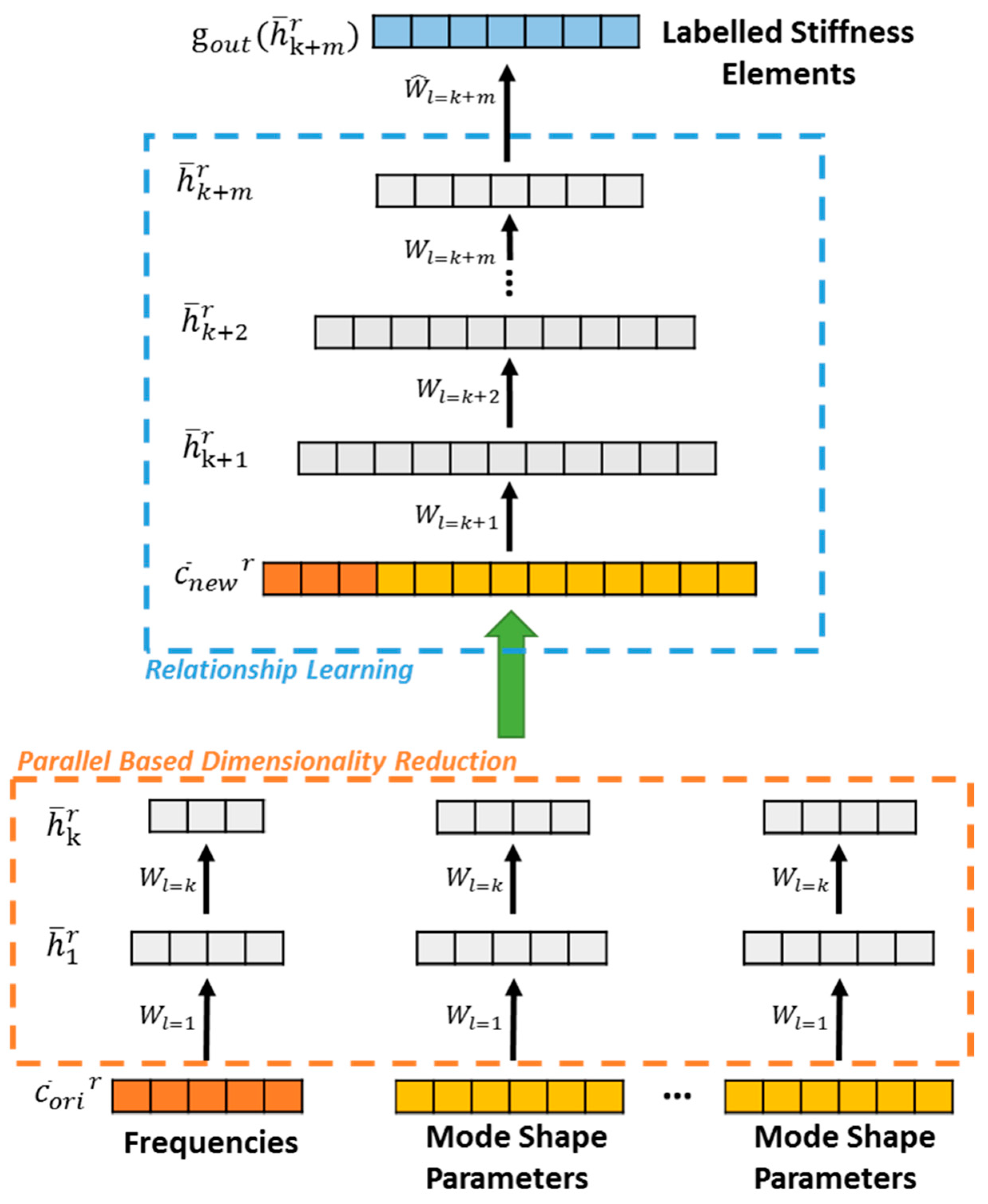
As described in Figure 2, each subset of input data is fed into a stacked sparse auto-encoder model with a deep neural network architecture for performing dimensionality reduction and they are conducted in parallel. In the proposed parallel structure, the 1st hidden layer of each sparse auto-encoder model is to learn the local essential distribution from each input subset. Then the 2nd to kth layers further compress the hidden features layer-by-layer, observed from the previous layer. Only the encoding layers of a stacked deep auto-encoder are shown in the dimensionality reduction component in Figure 2. Depending on the problem complexity, the “deep architecture” can be extended deeper to match the problem complexity. The brief introductions on the sparse auto-encoder, sparse activation function and the formulation of objective functions for the parallel dimensionality reduction component are provided in Section 2.2.2 and Section 2.2.3, respectively.
2.2.2. Sparse Auto-Encoder
An auto-encoder is trained to reconstruct its input to its output [35]. However, if an auto-encoder succeeds in simply copying its input to its output, it may not extract any useful features. A sparse auto-encoder is an extension of the auto-encoder whose training criterion involves a sparsity penalty term on the hidden neurons inspired by sparse coding [9], along with the reconstruction error. By regularizing the auto-encoder to be sparse, it must respond to unique statistical features of the training dataset, rather than purely acting as an identity function [35]. Hence, training a sparse auto-encoder to perform reconstruction task can produce useful features.
The detailed formulation of sparsity penalty term will be explained further here. Let denotes the activation of hidden neuron when the network is given the ith input . Then, the average activation of hidden neuron that averaged over the whole training datasets can be expressed as:
where m is the number of samples. The constraint is enforced as:
where is a sparsity parameter that needs to be pre-determined as a small value (typically close to zero). In this process, the average activation of each hidden neuron j would be close to zero. In the other words, the hidden neurons are mostly ‘inactive.’ To achieve this, an extra penalty term is introduced to the optimization objective function that penalizes if it deviates significantly from as below:
where is the Kullback-Leibler (KL) divergence [36]: a measure of the similarity between two distributions and . In the other words, as diverges from , the KL divergence increases monotonically. Hence the sparsity penalty term can be formulated as below:
where r is the number of neurons in the hidden layer and the index is summing over the hidden neurons in the network.
2.2.3. Sparse Activation Function and Cost Function
Inspired by the work of SAF [34], sparse auto-encoder can also be used for performing dimensionality reduction with learning a sparse representation of modal data. Meanwhile, the learnt representation is considered to be not only sensitive to structural local damage but also robust to system uncertainties and measurement noise. One way to achieve actual zeros in the hidden representations is to use Rectified Linear Unit (ReLUs) [27] as encoder activation function over the alternative non-sparse activation functions, such as ‘tanh’ and ‘sigmoid’, in the auto-encoder. In this way, a ReLU can indirectly control the sparsity in the representation [35]. For the proposed framework, we implement the sparse auto-encoder in the parallel dimensionality reduction component to explore the advantages of our method in comparison with SAF. The reconstruction cost function of layer in each parallel block (Figure 2) is defined as follows.
where
Equation (7) denotes an overall cost function, which includes a Mean Squared Error (MSE) loss term and a weight decay regularization term, where W is the weight matrix and is the bias vector. To optimize the parameters W and , usually MSE is employed as the loss function in Equation (8), where p = {1… k} with k being the number of hidden layers in dimensionality reduction component for each block, N is the total number of training samples. represents the encoder function for layer where a ReLU is used to impose sparsity on the hidden representation. However, applying too strong sparsity may hurt inference performance, since it reduces the effective capacity of the model. Therefore, a sparse regularization term defined in Equation (6) is added to Equation (7), where is the hyper-parameter to control the trade-off between the reconstruction loss and the applied constraints on the solution. is the decoder function for layer and it is set to be a linear activation function to reconstruct the real values of input to output is the compressed hidden feature vector taken from layer in the sample with . Equation (9) is a L2-weight decay regularization term, where is an element in weight matrix W and denotes the number of hidden neurons in layer . The L2-weight decay term is added to avoid over-fitting by shrinking the weights on features. In Equation (7) a hyper-parameter is utilized to penalize the weight decay term. It is reminded that we carry out dimensionality reduction separately in the proposed model for simplicity with assumption that all blocks have the same number of layers.
An unsupervised layer-wise pre-training based on sparse auto-encoders is performed for all layers of every block in the parallel structure. The sparse hidden representation of each pre-trained auto-encoder is taken out at the input for the next layer. Finally, the features learnt from kth layer of each block are concatenated as new input vector and fed into a nonlinear relationship learning component as described in Section 2.2.4.
2.2.4. Relationship Learning
A stacked deep auto-encoder with multiple non-linear layers (encoding layers) followed by a linear output layer is formed as the relationship learning part in Figure 2. After finishing dimensionality reduction for all the subsets of input, the hidden features taken from the last encoding layer of each auto-encoder model for all the samples are concatenated as one vector to form a new feature vector. is considered to be a better representation of the original input and it will be fed into the relationship learning part for learning the nonlinear regression against the output (labelled stiffness elements).
A supervised pre-training scheme is performed layer by layer via multiple simple auto-encoders in this part to initialize the layer weights that are close enough to a good solution. The cost function of sth layer for nonlinear relationship learning is defined as follows.
where
Equation (10) describes an overall cost function, which includes a L2-weight decay term expressed similarly in Equation (9). Equation (11) denotes the MSE loss function, where s = {1…m} expresses m layers in the proposed relationship learning model. and are the encoder and decoder mapping functions respectively as mentioned in previous section. is the hidden feature vector extracted from relationship learning layer for the rth sample where . This criterion (10) is used to minimize the difference between the hidden features and the labelled outputs layer by layer. The hidden feature vector, which is in a lower dimensional representation of our original input from each previous layer, compressed gradually and trained to regress to the target.
When the pre-training for relationship learning is completed, all the encoding layers are stacked together followed by a linear regression output layer forming the stacked deep auto-encoder model (see Figure 2) for fine-tuning. The final objective function is defined as:
where is the predicted output vector through all layers in the relationship learning model as shown in Figure 2.
In summary, the frequencies and mode shapes are trained as input to the proposed framework while the stiffness parameters are the output vector. The relationship between input and output is learned by the proposed framework via two stages as mentioned in Section 2.2.1 and Section 2.2.2 respectively. Though the structure of the deep learning framework has changed in this paper, the optimization process is similar as the original one [2] with different cost functions. For completeness, we give a brief description for training and testing as below.
- Training: the training of this framework is complete via parallel dimensionality reduction and relationship learning.
- ○
- Perform dimensionality reduction for several input datasets (e.g., , ) in parallel. An unsupervised pre-training scheme is conducted for each layer of every block via a sparse auto-encoder.
- ○
- Obtain learnt features from layer of each block and concatenate them as new input vector .
- ○
- Feed into the next component named relationship learning as new input feature vector. A supervised pre-training scheme is performed layer by layer to train the to regress to the labelled stiffness elements .
- ○
- Finally, perform fine-tuning for relationship learning component by jointly optimizing all layers to achieve an improved accuracy of the proposed framework.
- Testing: after training, the weights are fixed for the proposed framework. Testing datasets are feed into the fixed framework and the performance is evaluated in terms of the MSE and the R-value.
Numerical studies will be presented in the next section.
3. Numerical Experiments
Numerical studies including the numerical model, data generation, data pre-processing as well as the evaluation of the proposed framework will be described in this section. With the consideration of the uncertainties in the finite element modelling and measurement noise effect in the data, the accuracy and efficiency of the proposed approach will be examined through the simulation data generated from the numerical finite element model.
3.1. Infrastructure Model and Numerical Model
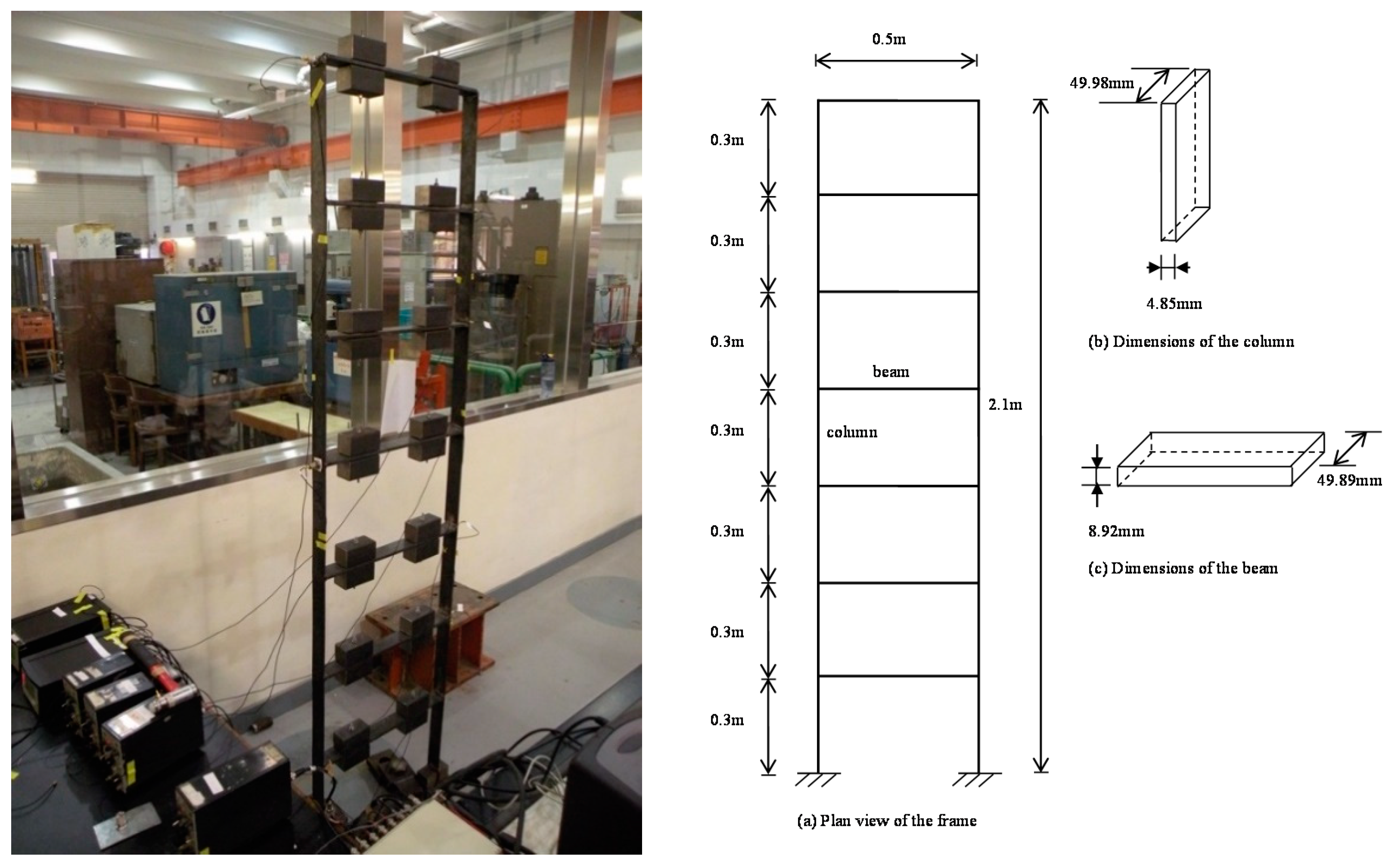
A seven-storey steel frame structure has been built in the laboratory at Curtin University and its frame dimensions are illustrated in Figure 3. Each storey is 0.3 m in height, composing up to 2.1 m for the total column height of the steel frame whereas the beam length of the steel frame is 0.5 m. The cross-sections of the column and beam elements are shown with dimensions of 49.98 mm × 4.85 mm and 49.89 mm × 8.92 mm respectively, while the corresponding measured mass densities of the column and beam elements are 7850 kg/m3 and 7734.2 kg/m3. Initial Young’s modulus of 210 GPa is applied to all members. The column and beam elements are connected continuously by welding at the top and bottom of the beam sections. The two columns at the bottom of the steel frame are welded onto a thick and solid steel plate which is fixed to the ground. In order to simulate the mass from the floor of a building structure, two pairs of mass blocks with each around 4 kg in weight are fixed at the quarter and three-quarter length of the beam in each storey.
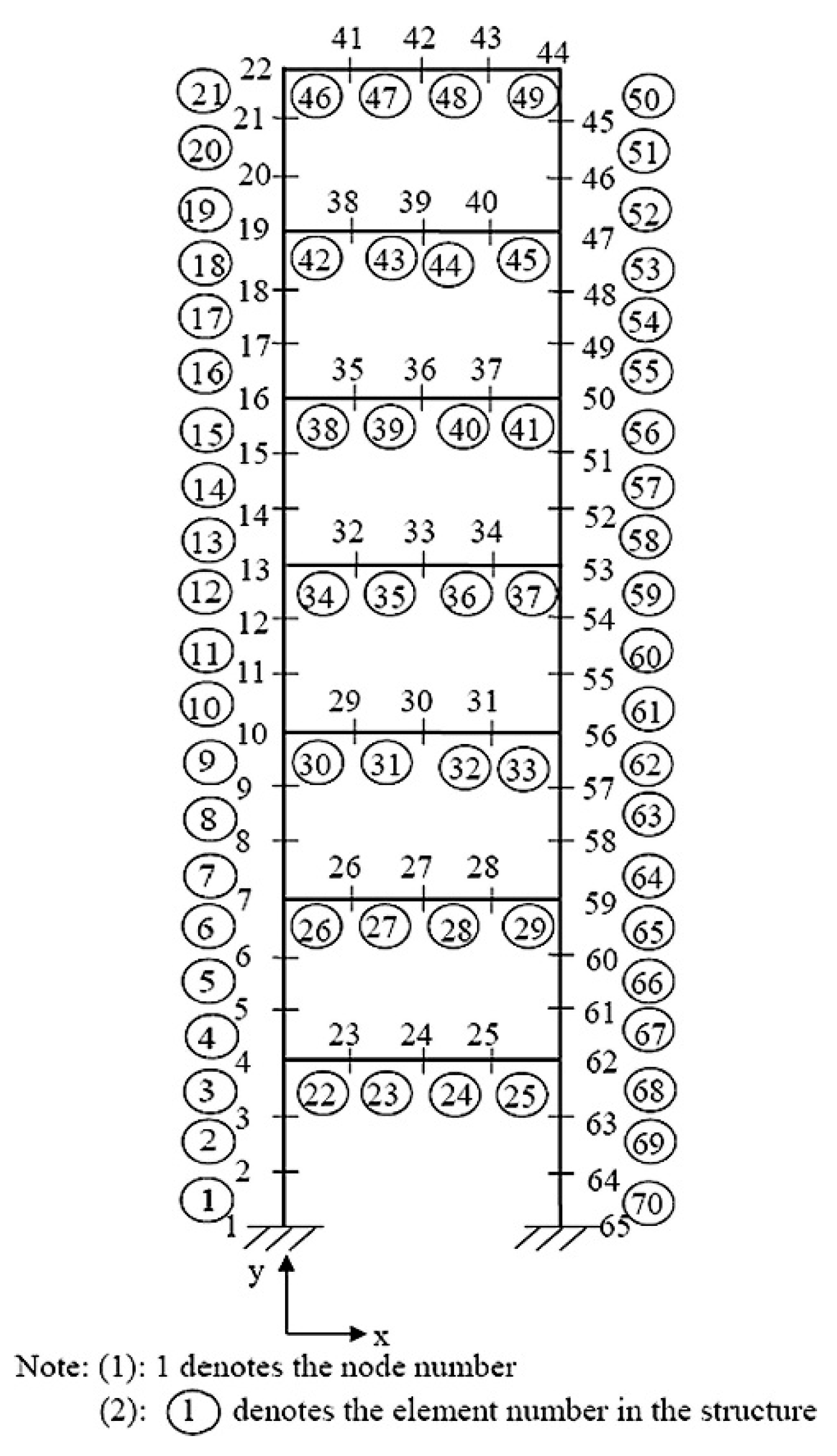
The finite element model of the whole frame structure is shown in Figure 4 which includes 65 nodes and 70 planar frame elements. The weights of steel blocks are loaded as concentrated masses at the corresponding nodes of the finite element model. Each node has three DOFs (two translational displacements x, y and a rotational displacement), contributing total 195 DOFs to the system. The translational (Node 1) and rotational (Node 65) restraints at the supports are expressed initially by the large stiffness of 3 × 10⁹ N/m and 3 × 10⁹ N·m/rad respectively. The initial finite element model updating has been executed to minimize the discrepancies between the analytical finite element model and the experimental model in the laboratory. This updated finite element model is adopted as the baseline model for generating the training, validation and testing data. The detailed model updating process can be referred to [4].
Notice that the data generated from FEM model could not totally replace the data from real structures. There are thousands of possibilities for the structural damage scenarios in real world. However, it is not practical to collect the data under such huge different damage scenarios from real civil structures. Therefore, the simulated data from FEM model is used in this paper to explore the damage identification problem.
3.2. Data Generation
Modal analysis is conducted using the finite element model above to generate the training dataset for both the input and output. As mentioned before, 7 frequencies and their corresponding mode shape parameters at 14 beam-column joints are measured and defined as the input. Seventy elemental stiffness parameters are generated as the output. The output is normalized to the range between 0 and 1, where 0 represents the totally damaged state whereas 1 represents the intact state of the structure element. For an instance, if a particular stiffness parameter is equivalent to 0.9, it indicates there is 10% stiffness reduction at this element.
Both single damage and multiple damage cases are considered in the 70 elements model. For single damage cases, there are total 2100 data sets generated from the baseline model based on the varying stiffness parameter of each element from 1, 0.99, 0.98… to 0.7 with leaving the other elements undamaged. Hence, for single element damage cases, 30 data sets are generated for each element with introducing a local damage. While 10,300 data sets are generated for multiple damage cases, two or more elements are considered as damage statuses with the stiffness parameter changing from 1, 0.99, 0.98… to 0.7. Meanwhile, the other elements are considered as intact statuses. Overall, 12,400 baseline data sets are generated based on the finite element model for training and validation.
Apart from the clean baseline datasets, noise datasets with measurement noise and uncertainty are also included in our study to further investigate the effectiveness and robustness of our proposed parallel structured model. For the noise datasets, 1% and 5% Gaussian noises are added to first seven frequencies and the associated mode shapes respectively with consideration of structural frequencies measured more accurately as reported in [21]. Besides, 1% uncertainty is considered in the stiffness parameters to simulate the finite element modelling errors. We expect to make the proposed model trained by these noise data more robust for predicting unknown data with measurement noises and uncertainties. Both baseline datasets and noise datasets will be used in comparison with the state-of-the-art models and the proposed model in the following experiments.
3.3. Data Pre-Processing
Since each mode shape subset belongs to a natural frequency; in addition, the input subsets of frequency features and mode shapes features are measured in different scales. Thus, to avoid the additional complexity in the input dataset, we first divide the entire dataset which including all the frequencies and mode shape parameters into 8 subsets. Each subset is normalized to the range of [0, 1] to serve the active range of ‘ReLU’.
For the output vector, each element lies in the range between 0 and 1, where 0 denotes the fully damaged state while 1 denotes the intact state. Since only a few elements are defined to be in damage situation in each sample and the stiffness parameter does not vary a lot in damage cases. Therefore, the stiffness parameters are normalized to the expanded range of [−1, 1] to serve the operating range of linear activation function at the output.
Then these pre-processed input and output datasets will be utilized to evaluate the proposed approach in the following sections.
4. Performance Evaluation
The above both baseline datasets and noise datasets are utilised to evaluate the performances of the proposed approach against the state-of-the-art model, for example, “Sparse Auto-encoder Framework (SAF)” [34]. For each of the model training, the pre-processed dataset is randomly split into training, validation and testing subsets according to the percentages 70%, 15% and 15% respectively. Finally, the Mean Squared Error (MSE) value and Regression value (R-value) are used to evaluate the quality of damage predictions of the proposed parallel model with the state-of-the-art models on the testing datasets. In particular, the MSE measures the distance between the estimated output of testing datasets from the proposed model and the labelled output. R-value represents the coefficient of correlation, which is used to measure the correlation between estimated output and labelled output. For our case, the higher R-value the more accurate of the proposed model. The details of proposed model architecture and evaluated performances are presented as follows.
In our experiment, the proposed parallel auto-encoder framework utilizes one hidden layer for each parallel block in dimensionality reduction component, with 9 hidden neurons in the 1st block for frequency data while 13 hidden neurons for the rest of 7 blocks for mode shape data. Since we implement sparse auto-encoders in this component, the number of hidden neurons are chosen carefully to allow the model to have more capacity for learning. To demonstrate the effectiveness of utilising many relationship learning layers, five hidden layers of having 90, 85, 80, 75 and 70 neurons respectively are defined in the relationship learning component. By using the decreasing number of hidden units in the hidden layers, the input vector is gradually compressed and regressed to the target vector. To perform a fair comparison with SAF, a simple proposed parallel model Para-AF-0 with the same number of hidden layers and neurons (90-80-70) as SAF in relationship learning component is also evaluated in this study.
The performances of using the SAF and the proposed approach are compared by investigating the MSE values and R-values on the testing datasets. Both baseline datasets and noise datasets with measurement noise and uncertainty effect are used. The performance evaluation results are shown as below.
As shown in Table 1, for the baseline dataset, MSE values obtained from SAF, Para-AF-0 and Para-AF are , and , respectively. Para-AF-0 has marginally improved the performance over SAF with a smaller MSE value for baseline dataset. Meanwhile, for noisy datasets, we can observe a 3% increment in R-value of Para-AF-0 versus SAF. They indicate that the proposed parallel dimensionality reduction has achieved the expected effectiveness by extracting features in parallel from multi-scale datasets. In addition, a significant increment (around 8%) in R-value is observed in Para-AF-0 against Para-AF, which shows the effectiveness of applying more relationship learning layers. For both datasets, the performances of these three methods show the same trend. Therefore, the proposed parallel method not only improves the effectiveness but also improves the noise robustness for damage detection/identification.
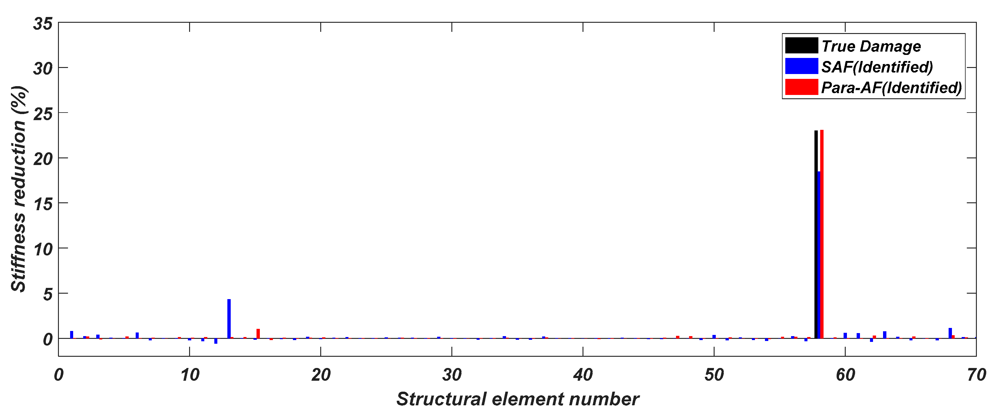
Since dealing with the noise dataset is much more challenging in the real-world, only this case will be further presented in the following comparisons. To further evaluate the quality of damage identification in terms of both magnitudes and locations, the prediction of a single damage case and a multiple damage case randomly selected from the testing datasets are shown in Figure 5 and Figure 6 respectively.
Firstly, for the single damage case, SAF can predict the true location of the single damage but fail to identify the true magnitude of the damage. In contrary, it can be observed clearly that the proposed method performs the best in damage identification with a very close identified stiffness reduction value against the true value. Besides, SAF produces a considerable false identification at the 13th element location of the structure. Therefore, the proposed method gives the higher accuracy in the prediction of damage pattern in terms of both the location and severity.
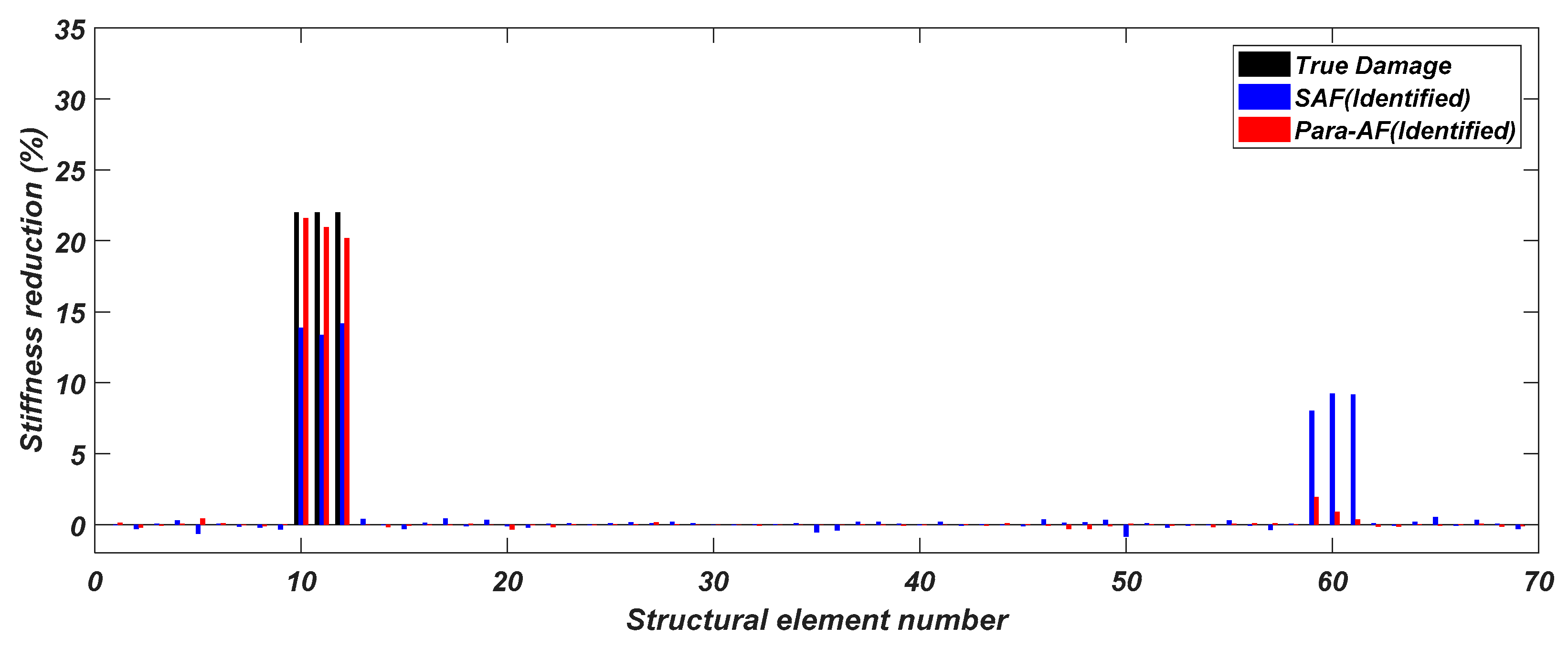
Furthermore, to evaluate the models for multiple structural damage cases, following example is chosen from the testing dataset and the predictions are shown in Figure 6. In comparison to the single damage case, the multiple damage cases need higher precision in identifying multiple damages’ locations and severities. It can be observed that the proposed approach performs much better in multiple damage cases too, with all the damage locations accurately detected. Furthermore, the identified stiffness reductions are very close to the true values with very small false identifications. In contrast, SAF is not working very well in identifying multiple damages with some significant false identifications appeared at non-damage locations.
As shown in the figures above, the identified stiffness reductions of the proposed method are superior to SAF in terms of both the magnitude and the location and this implies the robustness of using the proposed approach in structural elemental stiffness predictions.
Therefore, it has been demonstrated that our proposed parallel based approach not only improves the effectiveness but also improves the robustness for damage detection/identification in structural health monitoring against the state-of-the-art approach.
5. Conclusions
In this paper, we proposed a parallel auto-encoder framework to achieve dimensionality reduction for multi-scale datasets with a parallel designed architecture and to learn the relationship between modal information and stiffness mass in structural health monitoring. The framework works via two main stages, parallel dimensionality reduction and relationship learning. In dimensionality reduction stage, a robust (scale-invariant and highly correlated) concatenated feature that preserves the necessary information of input modal information is learned. In the relationship learning stage, the concatenated feature is utilized as the new input that feeds into a deep auto-encoder for learning the relationship between the stiffness parameters. We have achieved much higher accuracy for predicting the unknown baseline and noise testing data comparing to the-state-of-the-art model.
Our future work will include but is not limited to: (1) Extend our framework for analysing more complex structures such as a bridge model; (2) Apply our framework for other tasks with multi-scale or multivariate datasets.
Author Contributions
Conceptualization, R.W, L.L. and J.L.; Methodology, R.W. and J.L.; Software, R.W.; Validation, L.L. and J.L.; Formal Analysis, R.W.; Investigation, R.W.; Resources, J.L.; Data Curation, R.W.; Writing—Original Draft Preparation, R.W.; Writing—Review & Editing, L.L. and J.L.; Visualization, R.W.; Supervision, L.L.; Project Administration, L.L.
Funding
This research received no external funding.
Acknowledgments
We would like to give our sincerely thanks Chathurdara Sri Nadith Pathirage in Curtin University for his support throughout this research.
Conflicts of Interest
The authors declare no conflict of interest.
References
- Farrar, C.R.; Worden, K. An introduction to structural health monitoring. Philos. Trans. R. Soc. A Math. Phys. Eng. Sci. 2007, 365, 303–315. [Google Scholar] [CrossRef] [PubMed] [Green Version]
- Fan, W.; Qiao, P. Vibration-based damage identification methods: A review and comparative study. Struct. Health Monit. 2011, 10, 83–111. [Google Scholar] [CrossRef]
- Pathirage, C.S.N.; Li, J.; Li, L.; Hao, H.; Liu, W. Deep Autoencoder Model for Pattern Recognition in Civil Structural Health Monitoring. In Proceedings of the International Conference on Quality, Reliability, Risk, Maintenance, and Safety Engineering, Jiuzhaigou, China, 25–28 July 2016. [Google Scholar]
- Friswell, M.; Mottershead, J.E. Finite Element Model Updating. In Structural Dynamics; Springer Science & Business Media: Dordrecht, The Netherlands, 1995. [Google Scholar]
- Mottershead, J.E.; Friswell, M.I.; Ng, G.H.T.; Brandon, J.A. Geometric parameters for finite element model updating of joints and constraints. Mech. Syst. Signal Process. 1996, 10, 171–182. [Google Scholar] [CrossRef]
- Teughels, A.; De Roeck, G. Structural damage identification of the highway bridge Z24 by FE model updating. J. Sound Vib. 2004, 278, 589–610. [Google Scholar] [CrossRef]
- Brownjohn, J.M.W. Structural health monitoring of civil infrastructure. Philos. Trans. R. Soc. A Math. Phys. Eng. Sci. 2007, 365, 589–622. [Google Scholar] [CrossRef] [PubMed] [Green Version]
- Jaishi, B.; Ren, W.-X. Damage detection by finite element model updating using modal flexibility residual. J. Sound Vib. 2006, 290, 369–387. [Google Scholar] [CrossRef]
- Yun, C.-B.; Yi, J.-H.; Bahng, E.Y. Joint damage assessment of framed structures using a neural networks technique. Eng. Struct. 2001, 23, 425–435. [Google Scholar] [CrossRef]
- Bakhary, N.; Hao, H.; Deeks, A.J. Damage detection using artificial neural network with consideration of uncertainties. Eng. Struct. 2007, 29, 2806–2815. [Google Scholar] [CrossRef]
- Rojas, R. Neural Networks: A Systematic Introduction; Springer: New York, NY, USA, 1996; ISBN 3-540-60505-3. [Google Scholar]
- Mehrjoo, M.; Khaji, N.; Moharrami, H.; Bahreininejad, A. Damage detection of truss bridge joints using Artificial Neural Networks. Expert Syst. Appl. 2008, 35, 1122–1131. [Google Scholar] [CrossRef]
- Yeung, W.T.; Smith, J.W. Damage detection in bridges using neural networks for pattern recognition of vibration signatures. Eng. Struct. 2005, 27, 685–698. [Google Scholar] [CrossRef]
- Hinton, G.E.; Salakhutdinov, R.R. Reducing the dimensionality of data with neural networks. Science 2006, 313, 504–507. [Google Scholar] [CrossRef] [PubMed]
- Bengio, Y. Learning deep architectures for AI. Found. Trends Mach. Learn. 2009, 2, 1–127. [Google Scholar] [CrossRef]
- Krizhevsky, A.; Sutskever, I.; Hinton, G.E. ImageNet Classification with Deep Convolutional Neural Networks. In Advances in Neural Information Processing Systems 25; Pereira, F., Burges, C.J.C., Bottou, L., Weinberger, K.Q., Eds.; Curran Associates, Inc.: Red Hook, NY, USA, 2012; pp. 1097–1105. [Google Scholar]
- Pinheiro, P.; Collobert, R. Recurrent Convolutional Neural Networks for Scene Labeling. In Proceedings of the 31st International Conference on Machine Learning, Beijing, China, 21–26 June 2014; pp. 82–90. [Google Scholar]
- Arel, I.; Rose, D.C.; Karnowski, T.P. Deep machine learning-a new frontier in artificial intelligence research [research frontier]. IEEE Comput. Intell. Mag. 2010, 5, 13–18. [Google Scholar] [CrossRef]
- Schmidhuber, J. Deep learning in neural networks: An overview. Neural Netw. 2015, 61, 85–117. [Google Scholar] [CrossRef] [PubMed] [Green Version]
- Abdeljaber, O.; Avci, O.; Kiranyaz, S.; Gabbouj, M.; Inman, D.J. Real-time vibration-based structural damage detection using one-dimensional convolutional neural networks. J. Sound Vib. 2017, 388, 154–170. [Google Scholar] [CrossRef]
- Jia, F.; Lei, Y.; Lin, J.; Zhou, X.; Lu, N. Deep neural networks: A promising tool for fault characteristic mining and intelligent diagnosis of rotating machinery with massive data. Mech. Syst. Signal Process. 2016, 72, 303–315. [Google Scholar] [CrossRef]
- Cha, Y.-J.; Choi, W.; Büyüköztürk, O. Deep Learning-Based Crack Damage Detection Using Convolutional Neural Networks. Comput. Civ. Infrastruct. Eng. 2017, 32, 361–378. [Google Scholar] [CrossRef]
- Cha, Y.-J.; Choi, W.; Suh, G.; Mahmoudkhani, S.; Büyüköztürk, O. Autonomous structural visual inspection using region-based deep learning for detecting multiple damage types. Comput. Civ. Infrastruct. Eng. 2017. [Google Scholar] [CrossRef]
- Kang, D.; Cha, Y.-J. Autonomous UAVs for Structural Health Monitoring Using Deep Learning and an Ultrasonic Beacon System with Geo-Tagging. Comput. Civ. Infrastruct. Eng. 2018. [Google Scholar] [CrossRef]
- Vincent, P.; Larochelle, H.; Lajoie, I.; Bengio, Y.; Manzagol, P.-A. Stacked denoising autoencoders: Learning useful representations in a deep network with a local denoising criterion. J. Mach. Learn. Res. 2010, 11, 3371–3408. [Google Scholar]
- Kan, M.; Shan, S.; Chang, H.; Chen, X. Stacked progressive auto-encoders (spae) for face recognition across poses. In Proceedings of the IEEE Conference on Computer Vision and Pattern Recognition, Columbus, OH, USA, 23–28 June 2014; pp. 1883–1890. [Google Scholar]
- Glorot, X.; Bordes, A.; Bengio, Y. Deep Sparse Rectifier Neural Networks. Aistats 2011, 15, 275. [Google Scholar]
- Doi, E.; Balcan, D.-C.; Lewicki, M.S. A theoretical analysis of robust coding over noisy overcomplete channels. Adv. Neural Inf. Process. Syst. 2006, 18, 307. [Google Scholar]
- Olshausen, B.A.; Field, D.J. Sparse coding with an overcomplete basis set: A strategy employed by V1? Vision Res. 1997, 37, 3311–3325. [Google Scholar] [CrossRef]
- Ranzato, M.; Poultney, C.; Chopra, S.; LeCun, Y. Efficient learning of sparse representations with an energy-based model. In Proceedings of the 19th International Conference on Neural Information Processing Systems, Doha, Qatar, 12–15 November 2012; pp. 1137–1144. [Google Scholar]
- Lee, H.; Battle, A.; Raina, R.; Ng, A.Y. Efficient sparse coding algorithms. In Advances in Neural Information Processing Systems; MIT Press Ltd.: Cambridge, MA, USA, 2007; pp. 801–808. [Google Scholar]
- Olshausen, B.A.; Field, D.J. Emergence of simple-cell receptive field properties by learning a sparse code for natural images. Nature 1996, 381, 607. [Google Scholar] [CrossRef] [PubMed]
- Erhan, D.; Courville, A.; Vincent, P. Why Does Unsupervised Pre-training Help Deep Learning? J. Mach. Learn. Res. 2010, 11, 625–660. [Google Scholar] [CrossRef]
- Pathirage, C.S.N.; Li, J.; Li, L.; Hao, H.; Liu, W.; Wang, R. Development and Application of a Deep Learning based Sparse Autoencoders Framework for Structural Damage Identification. Struct. Health Monit. 2018. submitted. [Google Scholar]
- Goodfellow, I.; Bengio, Y.; Courville, A.; Bengio, Y. Deep Learning; MIT Press Cambridge: Cambridge, MA, USA, 2016. [Google Scholar]
- Joyce, J.M. Kullback-leibler divergence. In International Encyclopedia of Statistical Science; Springer: Berlin, Germany, 2011; pp. 720–722. [Google Scholar]
Figure 1.
Proposed parallel based sparse auto-encoder framework.

Figure 2.
Proposed parallel auto-encoder model.

Figure 3.
Laboratory steel frame model and the dimensions of the steel frame structure.

Figure 4.
Finite element model of the steel frame structure.

Figure 5.
Damage identification results of a single damage case from SAF and the proposed approach.

Figure 6.
An example of multiple damage identification of SAF and the proposed approach.


Table 1.
Evaluation results for SAF and the proposed methods.
| Methods | Baseline Dataset | Noise Dataset | ||
|---|---|---|---|---|
| MSE | R-Value | MSE | R-Value | |
| SAF | 0.993 | 0.792 | ||
| Para-AF-0 | 0.994 | 0.823 | ||
| Para-AF | 0.996 | 0.901 | ||
© 2018 by the authors. Licensee MDPI, Basel, Switzerland. This article is an open access article distributed under the terms and conditions of the Creative Commons Attribution (CC BY) license (http://creativecommons.org/licenses/by/4.0/).
Share and Cite
MDPI and ACS Style
Wang, R.; Li, L.; Li, J. A Novel Parallel Auto-Encoder Framework for Multi-Scale Data in Civil Structural Health Monitoring. Algorithms 2018, 11, 112. https://doi.org/10.3390/a11080112
AMA Style
Wang R, Li L, Li J. A Novel Parallel Auto-Encoder Framework for Multi-Scale Data in Civil Structural Health Monitoring. Algorithms. 2018; 11(8):112. https://doi.org/10.3390/a11080112
Chicago/Turabian StyleWang, Ruhua, Ling Li, and Jun Li. 2018. "A Novel Parallel Auto-Encoder Framework for Multi-Scale Data in Civil Structural Health Monitoring" Algorithms 11, no. 8: 112. https://doi.org/10.3390/a11080112
Note that from the first issue of 2016, this journal uses article numbers instead of page numbers. See further details here.