Improved Parameter Identification Method for Envelope Current Signals Based on Windowed Interpolation FFT and DE Algorithm

Abstract

Envelope current signals are increasingly emerging in power systems, and their parameter identification is particularly necessary for accurate measurement of electrical energy. In order to analyze the envelope current signal, the harmonic parameters, as well as the envelope parameters, need to be calculated. The interpolation fast Fourier transform (FFT) is a widely used approach which can estimate the signal frequency with high precision, but it cannot calculate the envelope parameters of the signal. Therefore, this paper proposes an improved method based on windowed interpolation FFT (WIFFT) and differential evolution (DE). The amplitude and phase parameters obtained through WIFFT and the envelope parameters estimated by the envelope analysis are optimized using the DE algorithm, which makes full use of the performance advantage of DE. The simulation results show that the proposed method can improve the accuracy of the harmonic parameters and the envelope parameter significantly. In addition, it has good anti-noise ability and high precision.

1. Introduction

The traditional electric energy meter usually works in sinusoidal linear load condition with high precision [1]. However, the use of semiconductors in electronic devices, such as compact fluorescent lamps, LEDs, and so on, introduces a lot of non-linearity and dynamic loads with a significant harmonic current content into electric power systems [2,3]. Additionally, the development of smart grids requires new energy sources, such as solar energy, wind power, etc. Furthermore, loads like electric vehicles will also be involved [4]. These non-linearity and dynamic loads, as well as the distributed powers, result in dynamic currents which present a transition form on some occasions. This dynamic current not only contains harmonics, but also has variable amplitudes, and is referred to envelope current in this paper. In addition, according to [5], it has been confirmed that traditional electric energy meters are not able to account for the presence of harmonics because the meter is quite sensitive to frequency variations.

Several approaches have been reported to analyze harmonics, including wavelet transform [6,7], neural network [8,9], multiple signal classification (MUSIC) algorithm [10,11], fast Fourier transform (FFT)-based method [12,13] and so on. So far, it has been a difficult and important research direction to find a suitable wavelet basis function for harmonic analysis [14,15]. The neural network method is a hot topic, but it is seldom used in practice, since it needs a large amount of sample training [16,17]. The MUSIC algorithm can only estimate harmonic frequencies, and the phase and amplitude information will be lost during the course of constructing a pseudo space spectrum [10]. The FFT-based method is the most widely used approach in practice, but it has the defects of spectrum leakage and picket-fence effect, and hence the windowed interpolation FFT (WIFFT) is applied to overcome these two defects [18,19]. Therefore, this paper will use WIFFT, a simple and effective method, to analyze the harmonic parameters of the envelope signal.

In order to analyze an envelope signal, both the harmonic parameters and envelope parameters need to be calculated. WIFFT is good at harmonic parameter analysis of stationary harmonic signal [19,20]. However, it has difficulty in handling the envelope signal under dynamic conditions, because it cannot analyze the envelope parameters. On the other hand, the envelope parameters can be obtained by an envelope analysis method (e.g., curve fitting), but the information on the harmonics is not involved in envelope analysis. It is obvious that the two processes, WIFFT and envelope analysis, are relatively independent. Therefore, this paper combines them for envelope signal analysis. Since the parameter values obtained by WIFFT and envelope analysis are not accurate enough, an appropriate optimization method should be used for further analysis. The envelope current signal is a nonlinear function of envelope parameters and harmonic parameters. Hence, parameter identification is essentially a nonlinear optimization problem. Differential Evolution (DE) is a kind of simple, fast, robust and global optimization algorithm, which has an obvious advantage in nonlinear and non-differentiable continuous space problems [21,22]. Therefore, this paper presents an improved parameter identification method for envelope signals based on the WIFFT and DE algorithms.

This paper is organized as follows: after some revision of the principle of WIFFT and DE algorithms, the idea and the implementation process of the combination method of WIFFT and DE are given. Then this paper analyzes the performance of this combination method through a simulation example. Finally, an envelope current signal of electric locomotive is applied to verify the simulation results.

2. Principles of WIFFT and DE Algorithms

2.1. Estimation of Harmonic Parameters by WIFFT

The WIFFT algorithm is an effective harmonic analysis method. The spectral characteristics of the window function can restrain the spectrum leakage, and the interpolation operation is not only a correction of the weighted process, but can also eliminate the picket-fence effect [23]. In electric energy metering, the Hanning window is often used, as described in [24]:

$$w(n)=\{\begin{array}{ll}0.5-0.5\cos \frac{2n\mathsf{\pi }}{N},& 0\le n\le N-1\\ 0,& n<0\mathrm{or}n>N-1\end{array}$$

(1)

Corresponding to the Hanning window, the formula of interpolation correction is:

$$\{\begin{array}{l}{\beta }_m=\frac{\left|X(k_{\mathrm{m}}+1)\right|}{\left|X(k_{\mathrm{m}})\right|},{\delta }_m=\frac{2{\beta }_{\mathrm{m}}-1}{1+{\beta }_{\mathrm{m}}}\\ f_m=(k_{\mathrm{m}}+{\delta }_{\mathrm{m}})\frac{f_s}{N}\\ A_m=\left|X(k_{\mathrm{m}})\right|\cdot \frac{2\mathsf{\pi }{\delta }_{\mathrm{m}}(1-{\delta }_{\mathrm{m}}^2)}{\sin (\mathsf{\pi }{\delta }_{\mathrm{m}})}\\ {\theta }_m=\mathrm{angle}[X(k_{\mathrm{m}})]-{\delta }_{\mathrm{m}}\mathsf{\pi }\frac{N-1}{N}\end{array}$$

(2)

In Formula (2), f_m, A_m and θ_m are the frequency, amplitude and phase parameter of m-th harmonic, respectively. k_m refers to the number of local maximum spectral line. $\left|X(k_{\mathrm{m}})\right|$ and $\mathrm{angle}[X(k_{\mathrm{m}})]$ are the amplitude and phase of spectral line k_m in the weighted signal, and β_m is the spectral peak ratio of two adjacent spectral lines.

2.2. Principle of DE Algorithm

Differential Evolution is a simple and efficient algorithm for global optimization over continuous spaces [25,26]. Let f(X) be the target function, the crossover rate is C, the scaling factor is F and the evolution generation is t. The steps of DE are as follows [27].

(1) Initialization step. Set the generation number t = 0 and randomly initialize a population of M individuals ${\mathit{P}}_t={[{\mathit{X}}_1(t),\dots ,{\mathit{X}}_M(t)]}^{\mathrm{T}}$ with ${\mathit{X}}_i(t)=[x_{i,1}(t),x_{i,2}(t),\dots ,x_{i,n}(t)]$.

(2) Mutation step. Generate a donor vector ${\mathit{Z}}_i(t)$ corresponding to the i-th target vector ${\mathit{X}}_i(t)$ via

$${\mathit{Z}}_i(t)={\mathit{X}}_{r1}+F\cdot ({\mathit{X}}_{r2}-{\mathit{X}}_{r3})$$

(3)

where $r_1,r_2,r_3$ are mutually exclusive integers randomly chosen from the range $[1,2,\dots ,M]$.

(3) Crossover step. Generate a trial vector ${\mathit{U}}_i(t)=[u_{i,1}(t),\dots ,u_{i,n}(t)]$ for the i-th target vector ${\mathit{X}}_i(t)$ according to

$$u_{i,j}=\{\begin{array}{ll}{z}_{i,j}& \mathrm{if}rand(0,1)<C\hspace{1em}\mathrm{or}\hspace{1em}j=j_{\mathrm{rand}}\\ x_{i,j}& \mathrm{otherwise}.\end{array}$$

(4)

where $j_{\mathrm{rand}}\in [1,2,\dots ,\mathrm{n}]$ is a randomly chosen index.

(4) Selection step. Evaluate the trial vector ${\mathit{U}}_i(t)$ through

$${\mathit{K}}_i(t)=\{\begin{array}{ll}{\mathit{U}}_i\left(t\right)& \mathrm{if}\hspace{1em}f({\mathit{U}}_i(t))\le f({\mathit{X}}_i(t))\\ {\mathit{X}}_i\left(t\right)& \mathrm{otherwise}\end{array}$$

(5)

If f(K_i(t)) ≤ ε or t = t_max, then output K_i(t) as the optimal solution. Otherwise, X_i(t + 1) = K_i(t) and return to step (2).

3. An improved Method Based on WIFFT and DE

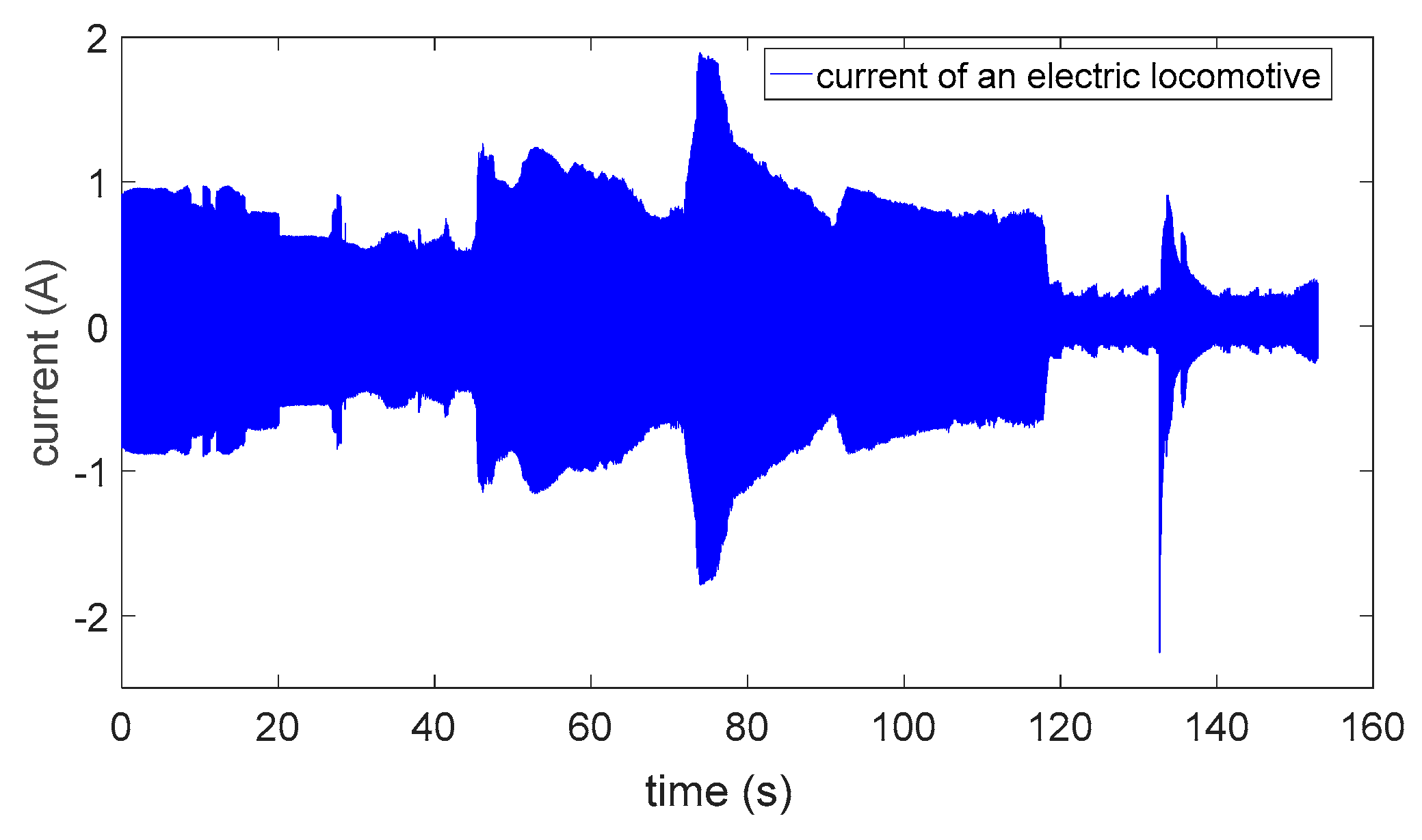
In practice, the envelope current signal is often presented in a trapezoidal envelope form. Figure 1 shows the current signal of an electric locomotive in about 152 s and it has 764,568 data points. Since the gentle exponential envelope and parabolic envelope can be regarded as an oblique envelope, this signal actually contains lots of trapezoidal envelopes.

In the trapezoidal envelope, the rise and fall part is the key to the analysis. Therefore, the trapezoidal envelope current signal is an oblique envelope one essentially. Therefore, this paper focuses on the parameter identification of the oblique envelope. The oblique envelope signal model takes this form,

$$x(t)=\left[(at+b)\cdot {\displaystyle \sum _{m=1}^M{A}_m\cos (2\mathsf{\pi }{f}_{m}t+{\theta }_m)}\right]+B_0$$

(6)

In Formula (6), f_m, A_m and θ_m represent the frequency, amplitude and phase of the harmonic signal, respectively. a is the slope of the oblique envelope, and b is the intercept.

The harmonic parameters can be estimated by Hanning WIFFT algorithm, which is presented in Formula (2). The DC component B₀ also corresponds to the DC parameter of FFT and the envelope parameter is given by linear fitting. In order to improve the estimation precision and the iterative efficiency, the pre-estimate value (a^*,b^*) obtained by the pretreatment of the envelope points can be used as the initial iterative value. The calculation process of the pre-estimate value is as follows.

(1) Search the envelope points of the signal. Find out the local maximum values and their times. Usually, the interval time between two adjacent local maximum points is about a power frequency cycle. The envelope curve is approximated as h(t) ≈ p₁t + p₂.

(2) In order to improve the stability of parameter estimation, the linear fitting method is used to solve p₁ and p₂. It is effective to eliminate the noise interference in the envelope due to the mean square error minimum criterion is employed. According to Formula (6), p₁ and p₂ take this form.

$$\{\begin{array}{c}{p}_1\approx a\cdot \Vert {\displaystyle \sum _m{A}_m\cos (2\mathsf{\pi }{f}_{m}t+{\theta }_m)}\Vert \\ p_2\approx b\cdot \Vert {\displaystyle \sum _m{A}_m\cos (2\mathsf{\pi }{f}_{m}t+{\theta }_m)}\Vert \end{array}$$

(7)

Therefore, the pre-estimate values of envelope parameters a^* and b^* are:

$$\{\begin{array}{c}{a}^{*}\approx \frac{p_1}{\Vert {\displaystyle \sum _m{A}_m\cos (2\mathsf{\pi }{f}_{m}t+{\theta }_m)}\Vert }\\ b^{*}\approx \frac{p_1}{\Vert {\displaystyle \sum _m{A}_m\cos (2\mathsf{\pi }{f}_{m}t+{\theta }_m)}\Vert }\end{array}$$

(8)

Therefore, the pre-estimate values of envelope parameters (a^*,b^*) and the harmonic parameters (A_m,θ_m) can be used to form the initial population of DE iteration. The initial population is

$$\mathit{P}={[{\mathit{X}}_1,{\mathit{X}}_2,\dots ,{\mathit{X}}_M]}^{\mathrm{T}}$$

(9)

where M is the population size and for an arbitrary individual, X = X_min + rand()·(X_max − X_min), where X_min = 0.5·[a^*,b^*,A_m,θ_m] and X_max = 1.5·[a^*,b^*,A_m,θ_m].

Root mean square error (RMSE) is taken as the target function f(X) of the DE algorithm, and it is defined as

$$f(\mathit{X})=RMSE=\sqrt{\frac{{\displaystyle \sum _n{\left[x(n)-x_c(n)\right]}^2}}{N}}$$

(10)

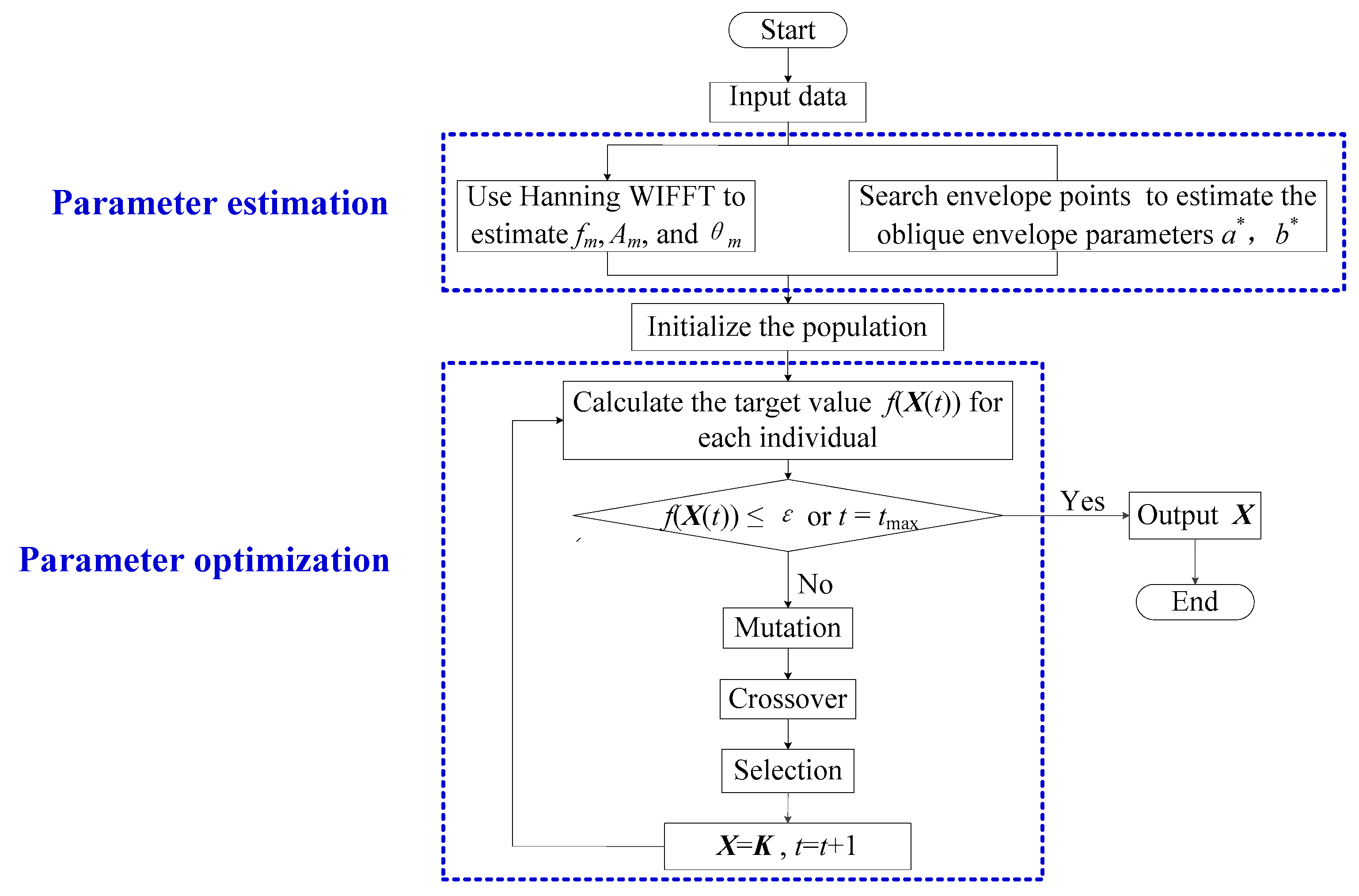
In Formula (10), x(n) is the sampling of the signal x(t), and x_c(n) is the reconstructed sequence by the identified parameters of the envelope signal, and N is the number of sequence. The smaller RMSE value indicates that the deviation of the actual waveform and the reconstructed signal waveform which is obtained by the combination algorithm is smaller, and the precision of parameter identification is also higher when using this combination method. Finally, the flow chart of the proposed method is shown in Figure 2.

4. Simulation of Parameter Identification for Envelope Current Signal

This section takes a given oblique envelope signal as an example and investigates the performance of parameter identification of the proposed method. Additionally, the measured current signal of an electric locomotive is used to analyze the applicability of the combination method in practical engineering.

4.1. Simulation of Oblique Envelope Signal with 3 Times Harmonic

The sampling sequence of the current signal model selected in this paper is as follows.

$$x(n)=(a\cdot n{T}_{\mathrm{s}}+b)\cdot {\displaystyle \sum _{m=1}^3{A}_m\cos (2\mathsf{\pi }\mathrm{m}{f}_0\cdot n{T}_{\mathrm{s}}+{\theta }_m)}+B_0$$

(11)

The fundamental frequency f₀ = 49.8 Hz, the phase θ are 60, 45 and 30, respectively, and the amplitude A_m are 100A, 5A and 10A, respectively. The envelope parameters are a = 0.5, b = 1 and the DC component is B₀ = 0.2. The sampling frequency is f_s = 5000 Hz, the sampling interval time T_s is 0.2 ms, and the total number of data points is N = 2000. The analysis is as follows.

4.1.1. The Analysis of Hanning WIFFT

Ignore the envelope parameters while analyzing the harmonics of this envelope signal. Therefore, the envelope signal is regarded as a virtual harmonic signal, and the calculated harmonic parameters are shown in

Table 1. Identification and errors of harmonic parameters of the oblique envelope signal.

Parameter	f0	A1	A2	A3	θ1	θ2	θ3
Calculated value	49.7987	109.9965	5.4999	11.0005	59.9290	44.7660	29.5623
Relative error (%)	0.0026	9.9965	9.9974	10.0050	0.1184	0.5200	1.4589

.

The comparison of the original signal and the reconstructed signal which calculated by WIFFT is shown in Figure 3.

Figure 3 indicates that for the harmonic parameters calculated by WIFFT, the error of amplitude is the largest (about 10%), the error of phase is about 1%, and the error of frequency is 0.0026%, which is the smallest. Furthermore, the change of envelope parameters a and b can still result in the consistent conclusion that is the frequency error is within 0.1%, but the amplitude error is large (up to 60% when a = 3). The results show that the precision of frequency estimation is extremely insensitive to envelope parameters while the amplitude is most sensitive because it is directly affected by the envelope parameters. Figure 3 also demonstrates that the signal reconstructed by the harmonic parameters is the equal-amplitude signal, which is the mean square approximation of the original signal. Although the RMSE is 4.1173, which seems smaller, it cannot reflect the amplitude change of the envelope signal. Therefore, WIFFT is not suitable to analyze the dynamic signal directly.

4.1.2. The Analysis of WIFFT and Envelope Parameters Estimation

The previous step, Hanning WIFFT, is employed to calculate the harmonic parameters. In addition, the signal envelope curve is used to estimate the envelope parameters a and b. The two steps are separated in this analysis. Therefore, the frequency and phase precision of harmonic parameter identification is consistent with the previous analysis. The process of envelope parameter estimation is as follows. The coefficients p₁ and p₂ are given by linear fitting of the envelope, and the envelope parameters a^* and b^* are given by Formula (8). For the simulation model, the harmonic amplitude parameter in the Formula (8) can be a set value which is able to investigate the performance of the fitting algorithm. Meanwhile, in the analysis of the actual measured signal, the amplitude parameter should be the estimated values computed by WIFFT algorithm. In addition, the following formula

$$(a\cdot n{T}_{\mathrm{s}}+b)\cdot {\displaystyle \sum _{m=1}^3{A}_m\cos (2\mathsf{\pi }\mathrm{m}{f}_0\cdot n{T}_{\mathrm{s}}+{\theta }_m)}=\frac{(a\cdot n{T}_{\mathrm{s}}+b)}{k}\cdot {\displaystyle \sum _{m=1}^{3}k\cdot A_m\cos (2\mathsf{\pi }\mathrm{m}{f}_0\cdot n{T}_{\mathrm{s}}+{\theta }_m)},\forall k\ne 0$$

(12)

indicates that the envelope parameters are correlated with the amplitude of harmonics. Hence, if the amplitude parameter has an error (the error of amplitude is about 10% in this example), the envelope parameters a and b, calculated by the Formula (8), still have errors even if the fitting process is zero-error. The envelope parameters identification of this example is shown in

Table 2. Identification and errors of envelope parameters of the oblique envelope signal.

Parameter	Valuation (Am Is the Set Value)	Relative Error (%)	Valuation (Am Is the Estimated Value)	Relative Error (%)
a*	0.7161	43.22	0.6510	30.2041
b*	0.9139	8.6111	0.8308	16.9166

.

Similarly, the reconstructed signal based on the estimated harmonic parameters and envelope parameters is shown in Figure 4.

It can be seen from Figure 4 that the reconstructed signal was able to reflect the change of envelope since it considers the envelope parameters a and b in this analysis model. However, according to Table 2, the estimation precision of envelope parameters is poor. The errors of a and b are 8.6% and 43.2%, respectively, even if the harmonic amplitudes are the set values. In addition, RMSE is 3.5218, which is better than the previous analysis. Therefore, the relative independent method of parameter identification is still insufficient, and it cannot be used in envelope signal analysis.

4.1.3. The Analysis of the Improved Method Based on WIFFT and DE Algorithms

The differential evolution algorithm is introduced to improve the precision in envelope parameter identification. It has no need to perofrm optimization for frequency, since the frequency estimation error calculated by WIFFT is very small. Therefore, this section only considers the optimization of envelope parameters a and b, amplitude parameters A_m and phase parameters θ_m. Set the aforementioned estimated value as the initial value of iteration, and DE algorithm parameters are as follows. The upper and lower bounds of the independent variables are 1.5 and 0.5 times of the initial value, respectively, the population size is 60, crossover factor is 0.4, crossover rate is 0.9 and the number of evolution generations is 100. Because the amplitude and envelope parameters are involved in the iteration, and they meet Formula (11) at the same time, it will result in different descriptions (a, b, A_m) of the same signal. Therefore, the following Formula (13) is proposed to calculate the envelope parameter error when analyzing the parameter identification.

$$Er{r}_{\_a}=\frac{a_{\_\mathrm{cal}}\cdot norm(A_{m\_\mathrm{cal}})-a_{\_\mathrm{exact}}\cdot norm(A_{m\_\mathrm{exact}})}{a_{\_\mathrm{exact}}\cdot norm(A_{m\_\mathrm{exact}})}$$

(13)

where a_{_cal} is the optimal value given by the differential evolution algorithm, a_{_exact} is the set value, norm(A_{m_cal}) is the amplitude norm of the optimal estimation which obtained by the DE algorithm, and norm(A_{m_exact}) is the norm of the set harmonic amplitude value. The dynamic parameter identification in this example is shown in

Table 3. Parameter identification and errors of the oblique envelope signal.

Parameter	a*	b*	A1	A2	A3	θ1	θ2	θ3
Valuation	0.3829	0.7656	130.6214	6.5348	13.0577	1.0490	0.7874	0.5246
Error (%)	0.0176	7.1951 × 10−4	/	/	/	0.1723	0.2580	0.1865

.

The signal reconstructed by the above identification parameters and errors is shown in Figure 5.

According to Figure 5, because of the DE algorithm, the error of envelope parameters is less than 0.0176% and the precision of phase calculation increases a lot—the maximum error decreases from 1.4589% to 0.258%. Furthermore, the approximation ability of the reconstructed signal is improved greatly. To be specific, the RMSE is only 0.0735, and the maximum absolute error is reduced from about 10 A to about 0.2 A, which means the precision is raised about 50 times. In addition, the computation time of WIFFT is 0.0492 s and the computation time of the proposed method is 1.8401s which is about 37 times of WIFFT. The computation time is the average of 30 times. The analysis result indicates that it is feasible to analyze the envelope signal through the combination method of WIFFT and DE algorithm.

Furthermore, the adaptability of this improved method in the case of noise is investigated. The difference of harmonic amplitudes has reached 26 dB, hence 40 dB, 50 dB and 60 dB noises are added to the signal for consideration. The results of parameter identification are as follows (

Table 4. Parameter identification and error of the noisy oblique envelope signals.

Parameter	a* (%)	b* (%)	RMSE	max[x(n) − xc(n)]
40dB	0.6669	0.0576	0.7762	2.5009
50dB	0.1529	0.0284	0.2557	1.0617
60dB	0.0568	0.0117	0.1082	0.3385

):

The results show that the method has good adaptability to noise, and it has a good precision even in these noisy cases.

4.2. Analysis of Envelope Current Signal of an Electric Locomotive

The following is a detailed analysis of an electric locomotive running current signal. The sampling frequency is f_s = 5000 Hz, and the total number of data points is N = 5000. The parameters of the DE algorithm are selected as for the previous example.

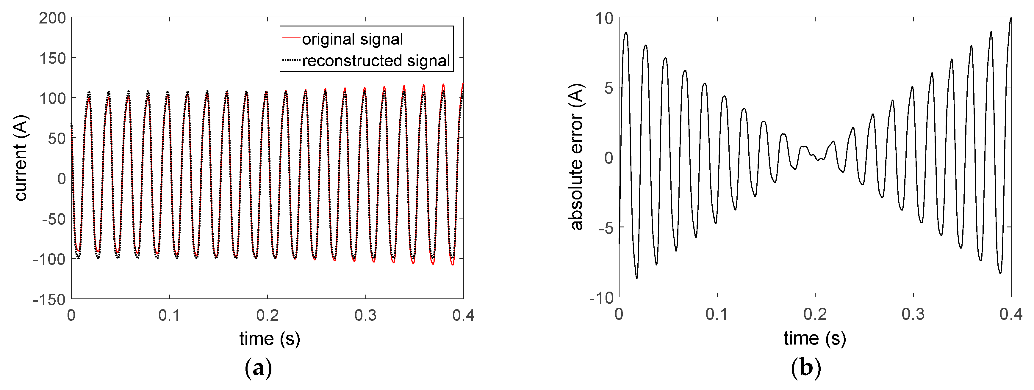
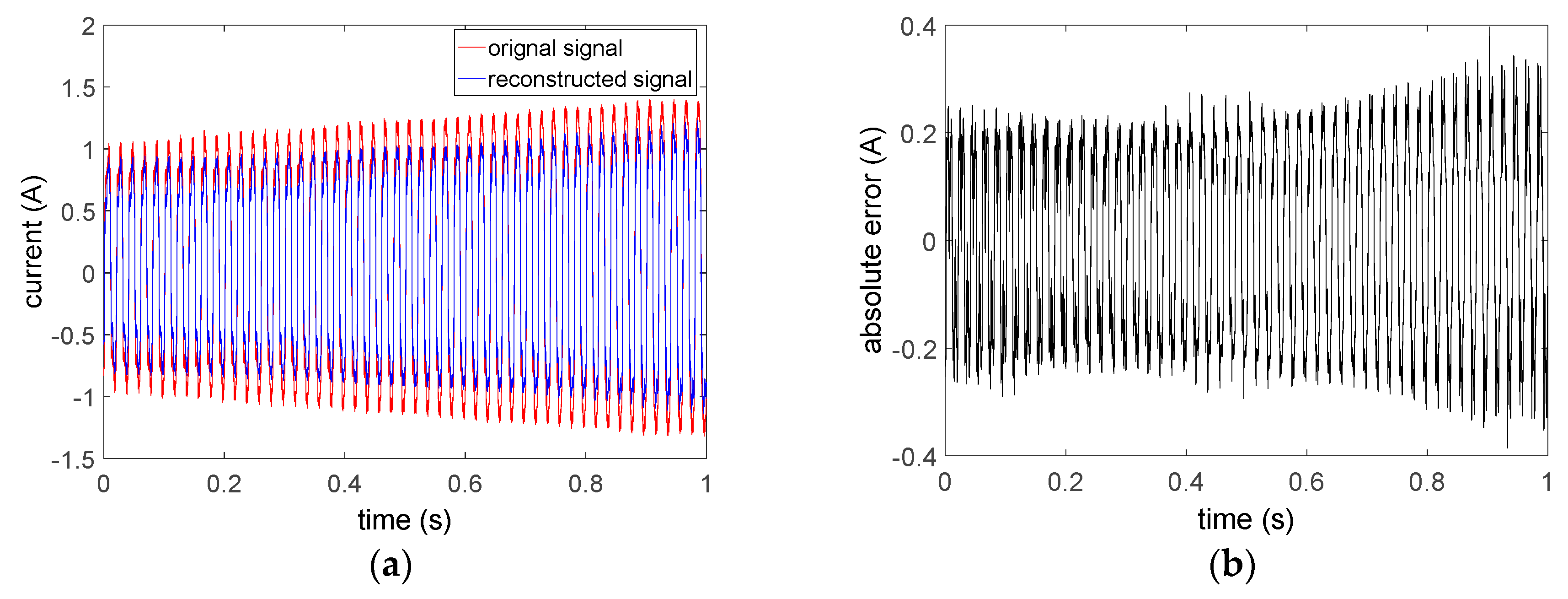
First of all, the reconstructed signal and absolute error are obtained by using Hanning WIFFT and the envelope parameter estimation method, as shown in Figure 6.

According to Figure 6, it is obvious that the actual measured current signal has the characteristic of an oblique envelope. Additionally, the larger prediction errors of envelope parameters result in significant difference between the reconstructed signal and the original signal. Furthermore, the RMSE is 0.1834 and the maximum absolute error is about 0.3966.

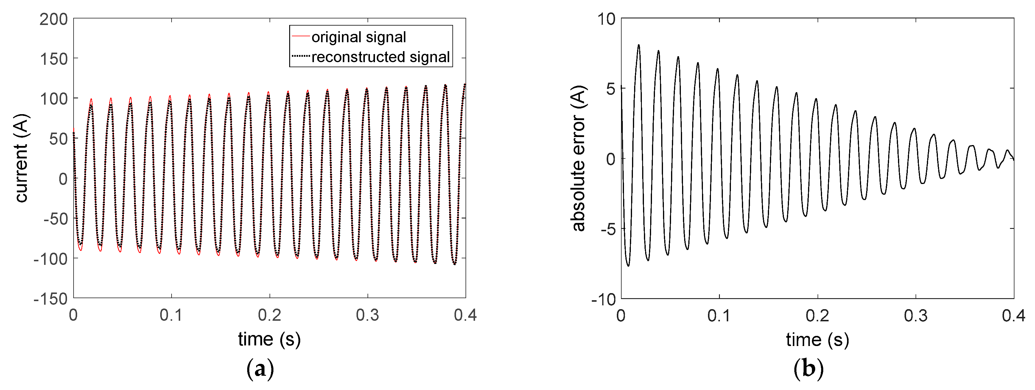
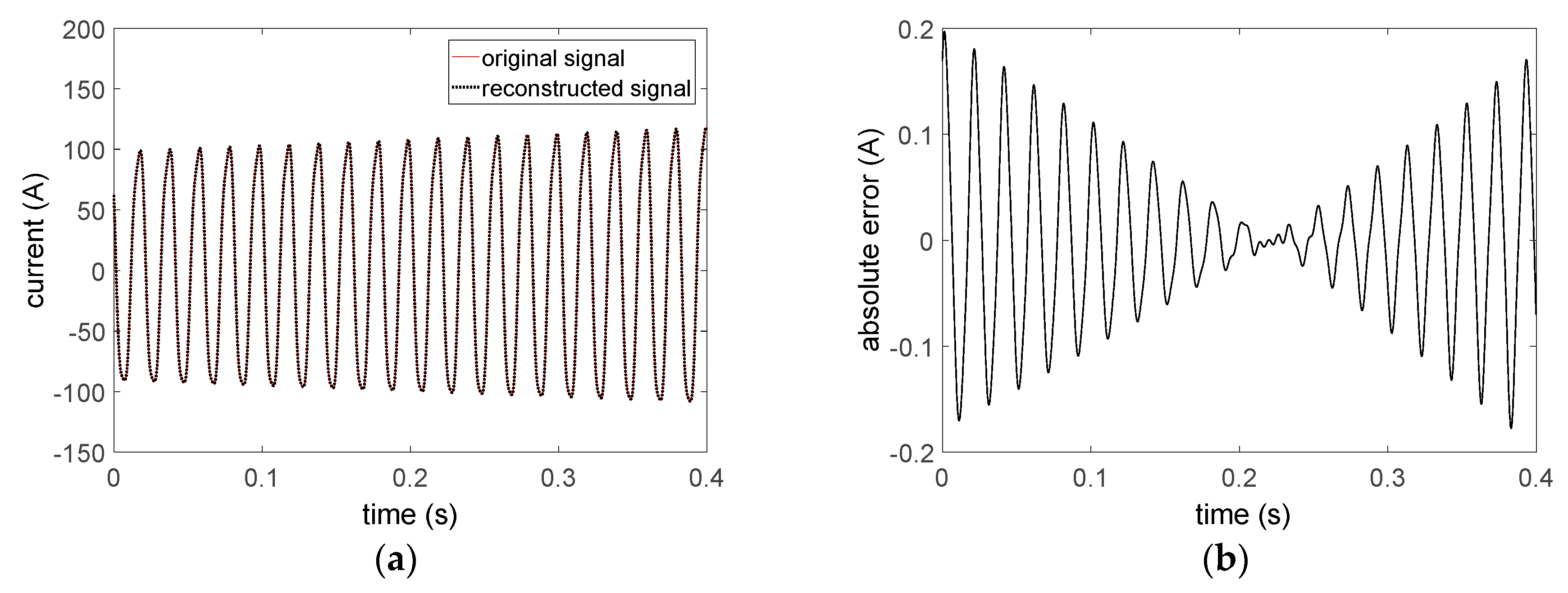
Then, the improved method based on WIFFT and DE is used in the analysis. The reconstructed signal and absolute error are shown in Figure 7.

Figure 7 demonstrates that the envelope parameters, harmonic amplitude and phase parameters are more accurate after the optimization of DE algorithm. In addition, the reconstructed signal is closer to the original signal, which means the precision of approximation is higher. Moreover, the RMSE is 0.0516 and the maximum absolute error is about 0.2116.

5. Results and Discussion

WIFFT is an effective approach to obtain harmonic frequencies. However, the hardest issue is to analyze the envelope parameters for an envelope signal. The simulation and experiment analysis show that the improved method based on WIFFT and DE algorithm can improve calculation precision of the envelope parameters greatly for an oblique envelope signal. Compared with the envelope parameters estimation method (based on Formula (7) and (8)), the relative error of envelope parameter a^* decreases from 30.2041% to 0.0176% and the relative error of b^* decreases from 16.9166% to 7.1951 × 10⁻⁴%. Besides, the simulation results indicate that the improved method has good adaptability to noise.

This paper mainly studies the parameter identification of the oblique envelope signal. It only requireds some simple modifications for the prediction formula of envelope parameters when this improved method is employed in the analysis of other types of envelope signal. Furthermore, an actual current signal not only contains the oblique envelope part, but also other kinds of envelopes, that is, this kind of signal is in fact the piecewise envelope signal. In order to analyze it precisely, the change point detection method of piecewise envelope signals should be investigated, which is an important follow-up work.

6. Conclusions

Aiming at the envelope current signal in the field of measurement, this paper proposes an improved method based on WIFFT and DE to analyze the harmonic parameters and envelope parameters of envelope signal. WIFFT can only result in frequency values with high precision. Its calculation results of amplitude and phase, as well as the envelope parameters obtained by envelope analysis method can be used as the initial value of the iteration and optimized by DE finally. In addition, the improved method can greatly improve the precision of parameter identification of the envelope signal. Moreover, it has a good anti-noise ability. These characteristics are verified by the example of an electric locomotive.

References

- Cataliotti, A.; Cosentino, V.; Nuccio, S. The Measurement of Reactive Energy in Polluted Distribution PowerSystems: An Analysis of the Performance of Commercial Static Meters. IEEE Trans. Power Deliv. 2008, 23, 1296–1301. [Google Scholar] [CrossRef]
- Brito, V.H.F.; Kume, G.Y.; Quinalia, M.S.; Sachetti, M.A.; Silva, R.P.B.; Souza, W.A.; Silva, L.C.P. Analysis of the influence of non-linear loads on the measurement and billing of electrical energy compared with the CPT. In Proceedings of the 2016 IEEE 17th International Conference on Harmonics and Quality of Power, Belo Horizonte, Brazil, 16–19 October 2016; pp. 617–622. [Google Scholar] [CrossRef]
- De Vasconcellos, A.B.; Carvalho, B.C.; Martins, W.C.; Anabuki, E.T.; Marques, L.T. The influence of the non-linearity of electric loads on capacitive compensation. In Proceedings of the 2012 IEEE 15th International Conference on Harmonics and Quality of Power, Hong Kong, China, 17–20 June 2012; pp. 880–886. [Google Scholar] [CrossRef]
- Gallardo-Lozano, J.; Milanés-Montero, M.I.; Guerrero-Martínez, M.A.; Romero-Cadaval, E. Electric vehicle battery charger for smart grids. Electr. Power Syst. Res. 2012, 90, 18–29. [Google Scholar] [CrossRef]
- Gallo, D.; Landi, C.; Langella, R.; Testa, A. On the Accuracy of Electric Energy Revenue Meter Chain Under Non-Sinusoidal Conditions: A Modeling Based Approach. In Proceedings of the 2007 IEEE Instrumentation & Measurement Technology Conference, Warsaw, Poland, 1–3 May 2007; pp. 1–6. [Google Scholar] [CrossRef]
- Tiwari, V.K.; Jain, S.K. Hardware Implementation of Polyphase-Decomposition-Based Wavelet Filters for Power System Harmonics Estimation. IEEE Trans. Instrum. Meas. 2016, 65, 1585–1595. [Google Scholar] [CrossRef]
- Dai, Y.; Xue, Y.; Zhang, J. A continuous wavelet transform approach for harmonic parameters estimation in the presence of impulsive noise. J. Sound Vib. 2016, 360, 300–314. [Google Scholar] [CrossRef]
- Garanayak, P.; Panda, G. Fast and accurate measurement of harmonic parameters employing hybrid adaptive linear neural network and filtered-x least mean square algorithm. IET Gener. Transm. Distrib. 2016, 10, 421–436. [Google Scholar] [CrossRef]
- Guellal, A.; Larbes, C.; Bendib, D.; Hassaine, L.; Malek, A. FPGA based on-line Artificial Neural Network Selective Harmonic Elimination PWM technique. Int. J. Electr. Power Energy Syst. 2015, 68, 33–43. [Google Scholar] [CrossRef]
- Sun, X.; Sun, L.; Zhao, S. Harmonic Estimation Algorithm based on ESPRIT and Linear Neural Network in Power System. Telkomnika 2016, 14, 47–55. [Google Scholar] [CrossRef]
- Nikolić, M.; Jovanović, D.P.; Lim, Y.L.; Bertling, K.; Taimre, T.; Rakic, A.D. Approach to frequency estimation in self-mixing interferometry: Multiple signal classification. Appl. Opt. 2013, 52, 3345–3350. [Google Scholar] [CrossRef] [PubMed]
- Su, T.; Yang, M.; Jin, T.; Flesch, R.C.C. Power harmonic and interharmonic detection method in renewable power based on Nuttall double-window all-phase FFT algorithm. IET Renew. Power Gener. 2018, 12, 953–961. [Google Scholar] [CrossRef]
- Jin, T.; Chen, Y.; Flesch, R.C.C. A novel power harmonic analysis method based on Nuttall-Kaiser combination window double spectrum interpolated FFT algorithm. J. Electr. Eng. 2018, 68, 435–443. [Google Scholar] [CrossRef]
- Weishi, M.; Jianhua, W.; Qing, K. Harmonic and inter-harmonic detection based on synchrosqueezed wavelet transform. In Proceedings of the 2016 IEEE Information Technology, Networking, Electronic and Automation Control Conference, Chongqing, China, 20–22 May 2016; pp. 428–432. [Google Scholar] [CrossRef]
- Liu, Z.; Geng, X.; Xie, Z.; Lu, X. The multi-core parallel algorithms of wavelet/wavelet packet transforms and their applications in power system harmonic analysis and data compression. Int. Trans. Electr. Energy Syst. 2016, 25, 2800–2818. [Google Scholar] [CrossRef]
- Murugan, A.S.S; Kumar, V.S. Determining true harmonic contributions of sources using neural network. Neurocomputing 2016, 173, 72–80. [Google Scholar] [CrossRef]
- Nascimento, C.F.; Jr, A.A.O.; Goedtel, A.; Dietrich, A.B. Harmonic distortion monitoring for nonlinear loads using neural-network-method. Appl. Soft Comput. J. 2013, 13, 475–482. [Google Scholar] [CrossRef]
- Wen, H.; Zhang, J.; Meng, Z.; Guo, S.; Li, F.; Yang, Y. Harmonic Estimation Using Symmetrical Interpolation FFT Based on Triangular Self-Convolution Window. IEEE Trans. Ind. Inform. 2015, 11. [Google Scholar] [CrossRef]
- Testa, A.; Gallo, D.; Langella, R. On the Processing of Harmonics and Interharmonics: Using Hanning Window in Standard Framework. IEEE Trans. Power Deliv. 2004, 19, 28–34. [Google Scholar] [CrossRef]
- Barros, J.; Diego, R.I. On the Use of the Hanning Window for Harmonic Analysis in the Standard Framework. IEEE Trans. Power Deliv. 2006, 21, 538–539. [Google Scholar] [CrossRef]
- Storn, R.; Price, K. Differential Evolution—A Simple and Efficient Heuristic for global Optimization over Continuous Spaces. J. Glob. Optim. 1997, 11, 341–359. [Google Scholar] [CrossRef]
- Rahnamayan, S.; Tizhoosh, H.R.; Salama, M.M.A. Opposition-Based Differential Evolution. IEEE Trans. Evolut. Comput. 2008, 12, 64–79. [Google Scholar] [CrossRef] [Green Version]
- Wen, H.; Dai, H.; Teng, Z.; Yang, Y.; Li, F. Performance Comparison of Windowed Interpolation FFT and Quasisynchronous Sampling Algorithm for Frequency Estimation. Math. Probl. Eng. 2014, 1–7. [Google Scholar] [CrossRef]
- Chen, K.F.; Mei, S.L. Composite Interpolated Fast Fourier Transform with the Hanning Window. IEEE Trans. Instrum. Meas. 2010, 59, 1571–1579. [Google Scholar] [CrossRef]
- Gosh, A.; Das, S.; Mallipeddi, R.; Das, A.K.; Dash, S.S. A Modified Differential Evolution with Distance-based Selection for Continuous Optimization in Presence of Noise. IEEE Access 2017, 5, 26944–26964. [Google Scholar] [CrossRef]
- Cai, Y.; Zhao, M.; Liao, J.; Wang, T.; Tian, H.; Chen, Y. Neighborhood guided differential evolution. Soft Comput. 2017, 21, 4769–4812. [Google Scholar] [CrossRef]
- Deb, A.; Roy, J.S.; Gupta, B. A Differential Evolution Performance Comparison: Comparing How Various Differential Evolution Algorithms Perform in Designing Microstrip Antennas and Arrays. IEEE Anten. Propag. Mag. 2018, 60, 51–61. [Google Scholar] [CrossRef]
Figure 1.
The current signal of an electric locomotive.
Figure 2.
The flow chart of the improved method based on WIFFT and DE algorithm.
Figure 3.
Simulation results of WIFFT: (a) Comparison of original signal and reconstructed signal; (b) Absolute error of original signal and reconstructed signal.
Figure 4.
Simulation results of WIFFT and envelope parameters estimation method: (a) Comparison of original signal and reconstructed signal; (b) Absolute error of original signal and reconstructed signal.
Figure 5.
Simulation results of the improved method based on WIFFT and DE algorithm: (a) Comparison of the original signal and reconstructed signal; (b) Absolute error of original signal and reconstructed signal.
Figure 6.
Analysis results of envelope current signal of an electric locomotive when employing the WIFFT and envelope parameter estimation method: (a) The comparison of original signal and the reconstructed signal; (b) Absolute error of original signal and reconstructed signal.
Figure 7.
Analysis results of envelope current signal of an electric locomotive when employing the improved method based on WIFFT and DE: (a) Comparison of the original signal and reconstructed signal; (b) Absolute error of original signal and reconstructed signal.