Robust Visual Tracking via Patch Descriptor and Structural Local Sparse Representation

Abstract

Appearance models play an important role in visual tracking. Effective modeling of the appearance of tracked objects is still a challenging problem because of object appearance changes caused by factors, such as partial occlusion, illumination variation and deformation, etc. In this paper, we propose a tracking method based on the patch descriptor and the structural local sparse representation. In our method, the object is firstly divided into multiple non-overlapped patches, and the patch sparse coefficients are obtained by structural local sparse representation. Secondly, each patch is further decomposed into several sub-patches. The patch descriptors are defined as the proportion of sub-patches, of which the reconstruction error is less than the given threshold. Finally, the appearance of an object is modeled by the patch descriptors and the patch sparse coefficients. Furthermore, in order to adapt to appearance changes of an object and alleviate the model drift, an outlier-aware template update scheme is introduced. Experimental results on a large benchmark dataset demonstrate the effectiveness of the proposed method.

1. Introduction

Visual tracking is a hot topic in the field of computer vision and has a wide range of applications, such as vision-based control [1], unmanned aerial vehicles [2], intelligent transportation [3], etc. Although some significant progress has been made in recent years, it still remains a challenging problem due to numerous appearance changes caused by factors, such as illumination changes, occlusion, scale variations, shape deformation, etc. Therefore, developing an effective appearance model is the key factor for robust tracking. Specifically, according to the used appearance model, current visual tracking methods can be roughly categorized into two classes: discriminative tracking and generative tracking.

In the generative tracking methods, the tracking problem is formulated as a search for regions most similar to the target model, and the information of the target is only used. Ross et al. [4] developed an online subspace learning model to account for appearance variation. In [5], a tracking algorithm based on a visual tracking decomposition scheme was proposed, and the observational model is decomposed into multiple basic observational models to cover a wide range of pose and illumination variation. Motivated by sparse representation in face recognition [6], Mei and Ling [7,8] formulated tracking as a sparse approximation problem. This method employs holistic representation schemes and hence does not perform well when target objects are heavily occluded. In [9], a tracking method based on the structural local sparse appearance model was proposed. This model exploits both partial information and spatial information, and handles occlusion by pooling across the local patches. In contrast to just use the target templates and the trivial templates to sparsely represent the target in [7,8], Guo et al. [10] proposed to represent the target object by a sparse set of target templates together with a sparse set of target weight maps. These weight maps contain the reliable structures of the target object. Lan et al. [11] proposed a multiple-sparse-representation-based tracker which learns the common and feature-specific patterns among multiple sparse representations for appearance modeling. In [12], Zhang et al. proposed a unified multi-feature tracking framework based on joint compressive sensing. Their framework can accept features extracted from identical spectral or different spectral images, and provide the flexibility to arbitrarily add or remove features.

On the contrary, the discriminative methods treat tracking as a binary classification problem, aiming to find a decision boundary that can best separate the target from the background. Unlike generative methods, the information of both the target and its background is used simultaneously. Avidan [13] used Adaboost to combine an ensemble of weak classifiers to form a strong classifier to do tracking. In [14], Grabner et al. proposed a semi-supervised online boosting algorithm to handle the drifting problem. Babenko et al. [15] proposed an online multiple instance learning (MIL) tracker, where samples are considered within positive and negative bags. Hare et al. [16] introduced a kernelized structured output support vector machine (Struck) for object tracking, which avoids the intermediate step to convert the estimated object position into a set of labeled training examples. Recently, the correlation filter (CF) based discriminative tracking methods have attracted a great deal of attention in tracking community. MOSSE [17] first introduced the CF to visual tracking. Subsequently, Heriques et al. exploited the circulant property of the kernel matrix [18], which was further improved using multi-channel HOG features [19]. Danelljan et al. [20] integrated adaptive scale estimations with the CF learning. The work of [21] performed complementary tracking that is robust to deformation and illumination variation. Inspired by the success of deep convolutional neural networks (CNNs) in object recognition and detection, several CF based trackers have been proposed to exploit CNN features [22,23,24].

In this paper, we pay attention to devising an effective appearance model and alleviating the model drift. Based on structural local sparse representation in [9], we design the patch descriptor to reflect the degree, to which each patch is contaminated with noise caused by appearance changes. Then, we model the appearance of an object by the combination of the patch descriptor and the patch sparse coefficients. Finally, we carry out tracking within the particle filter framework. Furthermore, we design an outlier ratio to describe the outlier degree of a target object. When the outlier ratio is larger than the threshold, we stop updating the template to alleviate the model drift.

The rest of this paper is organized as follows. Section 2 reviews the related work. In Section 3, we first describe target region division, then introduce structural local sparse representation, and finally detail the design of patch descriptor. In Section 4, we present our tracking method within the particle filter framework. Section 5 gives the template update scheme. Experimental results and comparisons are shown in Section 6. This paper concludes with Section 7.

2. Related Work

Visual tracking is one of the most challenging problems in computer vision. In order to give the context of our work, we briefly review the works most related to ours: patch-based tracking methods and strategies for alleviating model drift. For more detailed information on visual tracking, readers may refer to [25,26] and the references therein.

2.1. Patch-Based Tracking Methods

Instead of learning a holistic appearance model, many patch-based tracking methods have been developed, in which the target is modeled as a small number of rectangular blocks. If the target is partially occluded and deformed, its remaining visible patches can still represent the target and provide reliable cues for tracking. In [27], Adam et al. divided the target into multiple image patches to handle partial occlusion, and the integral image is used for feature extraction. Kwon and Lee [28] presented a local patch-based appearance model to address tracking of a target whose geometric appearance is drastically changing over time. An adaptive structural local sparse appearance model was proposed in [9], which handles occlusion by pooling across the local patches. Zhang et al. [29] matched local patches from multiple frames jointly by considering their low-rank and sparse structure information, which can effectively handle patch appearance variations due to occlusion or noise. In order to effectively handle deformation and occlusion, Cai et al. [30] designed a dynamic graph based tracker. They oversegment the target into several parts and then model the interactions between neighboring parts. Both the appearances of local parts and their relations are incorporated into a dynamic undirected graph. In [31], a patch-based tracking method with cascaded regression was proposed, which exploits the spatial constraints between patches by implicitly learning the shape and deformation parameters of the object in an online fashion. Sun et al. [32] proposed a fragment-based tracking method with consideration of both temporal continuity and discontinuity information, which exploits both foreground and background information to detect the possible occlusion. With the kernelized CFs, Li et al. [33] proposed a patch-based tracking method to handle challenging situations, where they employ the reliable patch particles to represent the visual target. A similar method can be found in [34].

Motivated by the aforementioned patch-based tracking methods, our approach also adopts a patch-based strategy to deal with challenging situations. However, different from existing methods, we design the patch descriptor to reflect the degree, to which each patch is contaminated with noise caused by appearance changes. The final tracked result is jointly determined by the patch descriptor and patch sparse coefficients.

2.2. Strategies for Alleviating Model Drift

The problem of corrupted or ambiguous samples is usually encountered in visual tracking, which deteriorates the representation power of tracking model, resulting in model drift. In order to handle this problem, various methods have been proposed. The work of [7,8] explicitly models the outliers in the corrupted target’s samples using trivial templates. In [15], online multiple instance learning was exploited to handle the label ambiguities caused by misaligned samples. Kalal et al. [35] developed a P-N learning method to estimate the tracker’s errors and correct them within a Tracking-Learning-Detection (TLD) framework. In [9], an update scheme based on the combination of sparse representation and incremental subspace learning was adopted to prevent model degradation. Zhang et al. [36] adopted multiple experts to address the model drift problem, which correct the past mistakes of online learning by allowing the tracker to evolve backward. The long-term correlation tracker (LCT) [37] alleviates model drift by modeling the temporal context correlation and the target appearance, using two regression models based on CFs. The tracking method in [38] adaptively learns the reliability of each training sample and downweighs the impact of corrupted ones. In [39], Shi et al. proposed a tracking algorithm based on Complementary Learner [21]. In order to reduce the risk of model drift, they construct a refiner model based on an online support vector machine (SVM) detector to update an incorrect prediction to a reliable position in case of low reliability of the current tracking result.

In this paper, in order to effectively reduce model drift caused by noisy updates, we design an outlier ratio to describe the outlier degree of a target object. When the outlier ratio is larger than the threshold, we stop updating the template.

3. Patch Descriptor and Structural Local Sparse Representation

3.1. Target Region Division

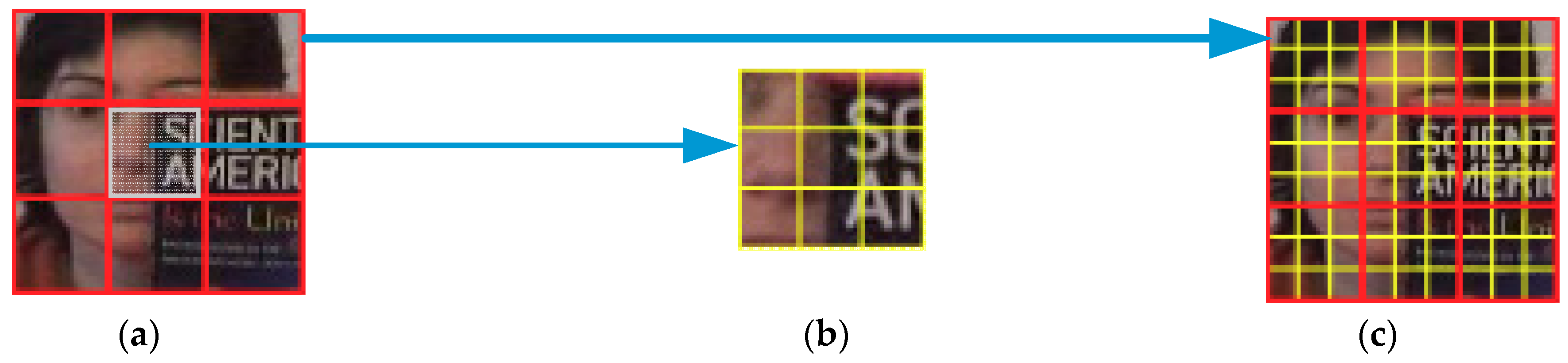
In this work, we normalized the target region into 36 × 36 pixels by applying affine transformation and extracting non-overlapped 12 × 12 local patches within the target region with 12 pixels as a step length, as shown in Figure 1a. Then, each local patch was further decomposed into several sub-patches again. The sub-patch size was 4 × 4 pixels, and the step length was 4 pixels, as shown in Figure 1b,c.

3.2. Structural Local Sparse Representation

Given a set of target templates $\mathit{T}=\{{\mathit{T}}_1,{\mathit{T}}_2,\dots ,{\mathit{T}}_n\}$, we divided each template in T into N non-overlapped local patches with a spatial layout (Figure 1a), and used these local patches as the dictionary to encode the local patches inside the candidate regions, i.e., $\mathit{D}=\left\{{\mathit{d}}_1,{\mathit{d}}_2,\dots ,{\mathit{d}}_{\left(n\times N\right)}\right\}\in {ℝ}^{d\times \left(n\times N\right)}$, where n is the number of target templates, d is the dimension of each patch vector, and N is the number of local patches sampled within one target region. Each column in D is obtained by ${\ell }_2$ normalization on the vectorized local image patches. For a target candidate, we divided it into N patches and turned them into vectors in the same way, which is denoted by $\mathit{Y}=\left\{{\mathit{y}}_1,{\mathit{y}}_2,\dots ,{\mathit{y}}_N\right\}\in {ℝ}^{d\times N}$. With the sparsity assumption, the local patches within the target candidate region can be sparsely represented as a linear combination of the dictionary D by solving the following ${\ell }_1$-regularized least squares problem:

$$\underset{{\mathit{b}}_i}{\min }\Vert y_i-\mathit{D}{\mathit{b}}_i{\Vert }_2^2+\lambda \Vert {\mathit{b}}_i{\Vert }_1, \mathrm{s}.\mathrm{t}.{\mathit{b}}_i\ge 0,$$

(1)

where $\lambda$ is the regularized parameter, ${\mathit{b}}_i\in {ℝ}^{\left(n\times N\right)\times 1}$ is the sparse coefficients of the i^th local image patch, and ${\mathit{b}}_i\ge 0$ means all the elements of ${\mathit{b}}_i$ are nonnegative. To represent local patch i at a certain position of the candidate, the sparse coefficients of the i^th patch are divided into n segments, i.e., ${\mathit{b}}_i^{\mathrm{T}}=[{\mathit{b}}_i^{(1)\mathrm{T}},{\mathit{b}}_i^{(2)\mathrm{T}},\dots ,{\mathit{b}}_i^{(\mathrm{n})\mathrm{T}}]$, according to the target templates, where ${\mathit{b}}_i^{(k)T}=\left[b_{\left(k-1\right)\times N+1},b_{\left(k-1\right)\times N+2},\dots ,b_{\left(k-1\right)\times N+N}\right]$ denotes the k^th segment of the coefficient ${\mathit{b}}_i$. Then, we weighed these coefficients to obtain ${\mathit{\nu }}_i$ for the i^th patch:

$${\mathit{\upsilon }}_i=\frac{1}{C}{{\displaystyle \sum }}_{k=1}^n{b}_i^{\left(k\right)}, i=1,2,\dots ,N$$

(2)

where ${\mathit{\nu }}_i$ is the sparse coefficient of the i^th local patch and C is a normalization term. Since one candidate target contains N local patches, all the vectors can form a square matrix V, $\mathit{V}=\left[{\mathit{v}}_1,{\mathit{v}}_2,\dots ,{\mathit{v}}_{\mathrm{N}}\right].$ The local appearance variation of a patch can be best described by the blocks at the same positions of the template. Therefore, we used the alignment-pooling method [9] and took the diagonal elements of the square matrix V as the final sparse coefficients of the local patches, i.e., $\mathit{f}=\mathrm{diag}\left(\mathit{V}\right)$, where $\mathit{f}=\left\{f_1,f_2,\dots ,f_{\mathrm{N}}\right\}$ is the sparse coefficient vector of all the local patches, i.e., $f_j$ means the sparse coefficient of the j^th local patch.

3.3. Patch Descriptor

Although the patch-based local sparse representation with the alignment-pooling process in [9] can capture both partial information and spatial information, it does not consider the different status among these patches, and this may influence the tracking performance when the appearance of patches of the target varies inconsistently. To address this issue, we assigned patch descriptors for different patches according to reconstruction errors of sub-patches using sparse representation.

The detailed analysis of target region division was given in Section 3.1. The dictionary base of each patch, obtained by clustering all the sub-patches in the patch at the same positions of the template, is $\mathit{P}=\left[p_1,p_2,\dots .,p_{\mathrm{K}}\right]\in {ℝ}^{\mathrm{z}\times \mathrm{K}}$, where z is the feature dimension of each dictionary, and K is the number of dictionaries. Let $\mathit{S}=\left[{\mathit{s}}_1,{\mathit{s}}_2,\dots ,{\mathit{s}}_{\mathrm{L}}\right]$ denote the vectorized sub-patches of each patch of a target candidate, where ${\mathit{s}}_i\in {ℝ}^{\mathrm{z}\times 1}$ is the i^th sub-patch, and L is the number of sub-patch. For each patch, when sparse coefficients of sub-patches in different patch were calculated, we used different dictionary base respectively, and its calculation formula was written as following:

$$\underset{x_i}{\min }\Vert {\mathit{s}}_i-\mathit{P}{x}_i{\Vert }_2^2+\gamma \Vert x_i{\Vert }_1, \mathrm{s}.t.x_{i>0}$$

(3)

where $x_i\in {ℝ}^{\mathrm{K}\times 1}$ is the sparse coefficient of i^th sub-patch in each patch, and $\mathsf{\gamma }$ is the regularized parameter. The reconstruction error of all the sub-patches in each patch can be calculated by the formula, ${\epsilon }_i=\Vert {\mathit{s}}_i-\mathit{P}{x}_i{\Vert }_2^2$, where ${\epsilon }_i$ is the reconstruction error of the i^th sub-patch in each patch. Let ${\delta }_i$ denote a factor of noise of the corresponding i^th sub-patch. It is defined by ${\delta }_i=\{\begin{array}{c}0, {\epsilon }_i<{\epsilon }_0\\ 1, otherwise\end{array}$, where ${\epsilon }_0$ is a threshold (${\epsilon }_0=0.04$ in our work). Each element of the patch descriptor $\rho =\left[{\rho }_1,{\rho }_2,\dots ,{\rho }_N\right]\in {ℝ}^{N\times 1}$ was defined as follows:

$${\rho }_j=1-{{\displaystyle \sum }}_{i=1}^L{\delta }_i/L, j=1,2,\dots ,N$$

(4)

where ${\rho }_j$ is the j^th patch descriptor representing the degree of noise pollution of the patch, and L is the number of sub-patch. The smaller the value of ${\rho }_j$ is, the more serious the patch will be corrupted.

4. Object Tracking

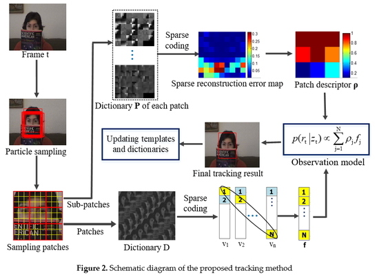
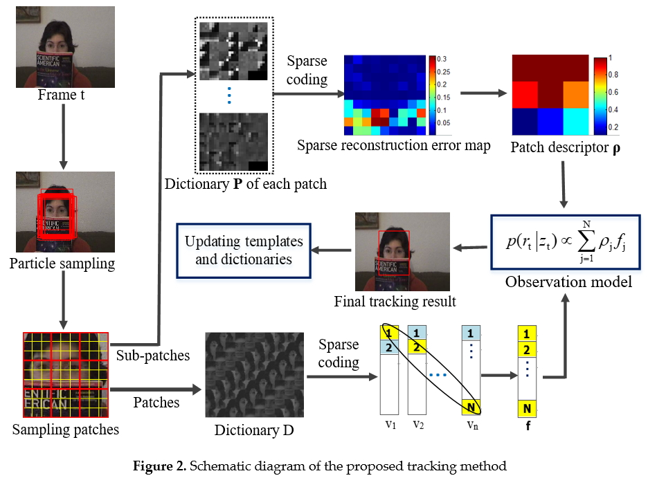
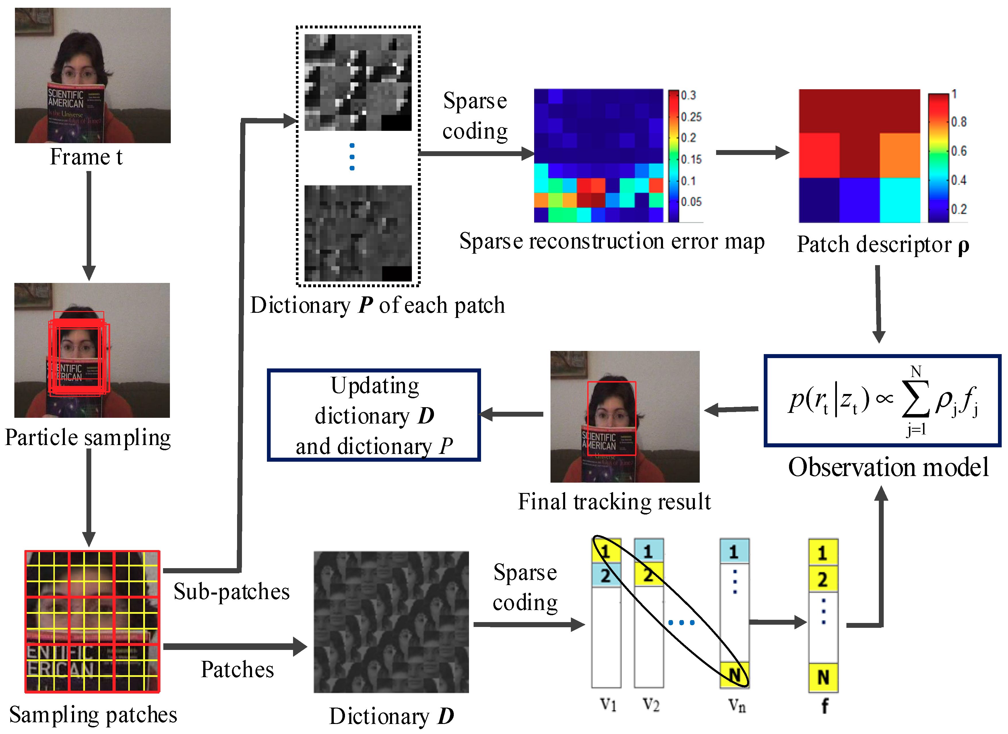
The basic flow of the proposed tracking algorithm is illustrated in Figure 2.

Our tracking method was carried out within the filter framework. At any time t, all target observations up to time t can be denoted by $R_t=\left\{r_1,r_2,\dots ,r_t\right\}$, and the state of a tracked object can be represented by $z_t$. The optimal state of the tracked object can be computed by the maximum a posteriori estimation, ${\widehat{z}}_t=\arg \underset{z_t^i}{\max }p(z_t^i|R_t)$, where $z_t^i$ is the i^th sample of the state $z_t$. The posterior probability was computed by the Bayesian theorem recursively:

$$p\left(z_t|R_t\right)\propto p\left(r_t|z_t\right)\int p\left(z_t|z_{t-1}\right)p\left(z_{t-1}|R_{t-1}\right)d{z}_{t-1}$$

(5)

where $\mathrm{p}\left(z_t|z_{t-1}\right)$ is the motion model between two consecutive states and $p\left(r_t|z_t\right)$ is the observation model. We modeled the motion of the object between two consecutive frames by affine transform. The state transition was formulated by random walk, i.e., $p\left(z_t|z_{t-1}\right)=\mathcal{N}\left(z_t:z_{t-1},\mathsf{\Sigma }\right)$, where $z_t=\left\{{\mathsf{\alpha }}_t,{\mathsf{\beta }}_t,{\mathsf{\mu }}_t,{\upsilon }_t\right\}$ denotes the x, y translations, scale and aspect ratio at time t, respectively. $\mathsf{\Sigma }=diag\left({\mathsf{\sigma }}_{\mathsf{\alpha }}^2,{\mathsf{\sigma }}_{\mathsf{\beta }}^2,{\mathsf{\sigma }}_{\mathsf{\mu }}^2,{\sigma }_{\upsilon }^2\right)$ is a diagonal covariance matrix, of which elements are the variances of the affine parameters.

The observation model $p\left(r_t|z_t\right)$ estimates the likelihood of observing $r_t$ at a state $z_t$. It plays an important role in object tracking, because it can reflect the variations of target appearance. In our algorithm, the observation model was defined by:

$$p\left(r_t|z_t\right)\propto {{\displaystyle \sum }}_{j=1}^N{\rho }_j{f}_j,$$

(6)

where the right side of the equation denotes the similarity between the candidate and the target based on the pooled feature $\mathit{f}$ and patch descriptor $\rho$. The candidate with the highest likelihood value is regarded as the tracking result.

5. Update Scheme

Object appearance often changes during tracking. We updated the target templates and dictionaries to adapt to the appearance changes every five frames. In [9], the sparse representation and subspace learning are used to update template:

$$\mathit{r}=\mathit{U}\mathit{q}+\mathit{e}=\left[U \mathit{I}\right]\left[\begin{array}{c}\mathit{q}\\ \mathit{e}\end{array}\right]$$

(7)

where r denotes the observation vector, U is the matrix composed of eigenvectors, q is the coefficient of eigenvectors, and e indicates the pixels in r that are corrupted or occluded. Assuming the error caused by occlusion and noise is arbitrary and sparse, Equation (7) can be solved by:

$$\underset{\mathit{c}}{\min }\Vert \mathit{r}-\mathit{H}\mathit{c}{\Vert }_2^2+\lambda \Vert c{\Vert }_1$$

(8)

where $\mathit{H}=\left[\mathit{U} \mathit{I}\right]$, $\mathit{c}={\left[\mathit{q} \mathit{e}\right]}^{\mathrm{T}}$ and $\mathsf{\lambda }$ is the regularization parameter. The reconstructed image $\mathit{U}\mathit{q}$ is then used for updating the template to be replaced.

In many tracking methods, the earlier tracking results are more accurate and should be stored longer than the newly tracking results in the template stack. In order to balance between the old and new templates, we introduced a cumulative probability sequence $\left\{0,1/\left(2^{n-1}-1\right),3/\left(2^{n-1}-1\right),\dots ,1\right\}$ and its each element means the update probability from the first template to the n^th template. We generated a random number according to the uniform distribution on the unit interval [0, 1] to choose a section in the sequence that the random number lies in and then determined which template should be replaced.

To further alleviate the problem of noise to be updated into the target templates, we introduced the outlier ratio $\eta$ to describe the outlier degree of a target object, which is denoted as:

$$\eta =1-{{\displaystyle \sum }}_{j=1}^N{\rho }_j/N.$$

(9)

We set two thresholds tr1 and tr2 to control the update of the template. If η < tr1, we updated the templates with this sample. If η > tr2, it meant that a significant part of the target object was corrupted, and we discarded this sample without update. If tr1 ≤ η ≤ tr2, it indicated that the target was partially corrupted. We then replaced the corrupted patches by its corresponding parts of the average observation $\mathit{\mu }$, and used this recovered sample for update. In order to recover the sample from corruptions, we constructed the sparse reconstruction error map of sub-patches and obtained the patch descriptor $\mathit{\rho }$. Then, the mask map $\mathit{M}={\left[M_1^T,M_2^T,\dots ,M_N^T\right]}^{\mathrm{T}}\in {ℝ}^{\left(d\times N\right)\times 1}$ can be obtained according to the patch descriptor $\mathit{\rho }$. If ${\mathit{\rho }}_i>0.7,M_i=1$, otherwise $M_i=0$. Hence, the recovered sample was modeled as:

$${\mathit{r}}_{\mathrm{new}}=\mathit{M}\odot \mathit{r}+\left(1-\mathit{M}\right)\odot \mathit{\mu }$$

(10)

where $\odot$ denotes elementwise multiplication, r is the partially corruption sample, and ${\mathit{r}}_{\mathrm{new}}$ represents the recovered sample.

The template update method is summarized in Algorithm 1. After the target templates update, we updated the dictionary D and the dictionary base P of each patch accordingly.

Algorithm 1. Method for template update.

Input: Observation vector r, eigenvectors U, average observation $\mathit{\mu }$, outlier ratio $\eta$, thresholds tr1 and tr2, template set T, the current frame f (f > n)

1: if mod(f,5) = 0 and $\mathsf{\eta }\le \mathrm{tr}2$ then

2: Generate a sequence of number in ascending order and normalize them into [0, 1] as the probability for template update;

3: Generate a random number between 0 and 1 which is for the selection of which template to be discarded;

4:  if $\eta <\mathrm{tr}1$

5:   Solve Equation (8) and obtain q and e;

6:   Add $\widehat{\mathit{r}}$ = Uq to the end of the template set T;

7:  else if $\mathrm{tr}1\le \eta \le \mathrm{tr}2$

8:   Solve Equation (10) and obtain the recovered sample ${\mathit{r}}_{\mathrm{new}}$;

9:   Solve Equation (8) and obtain q and e;

10:   Add ${\widehat{\mathit{r}}}_{\mathrm{new}}$ = Uq to the end of the template set T;

11:  end if

12: end if

Output: New template set T

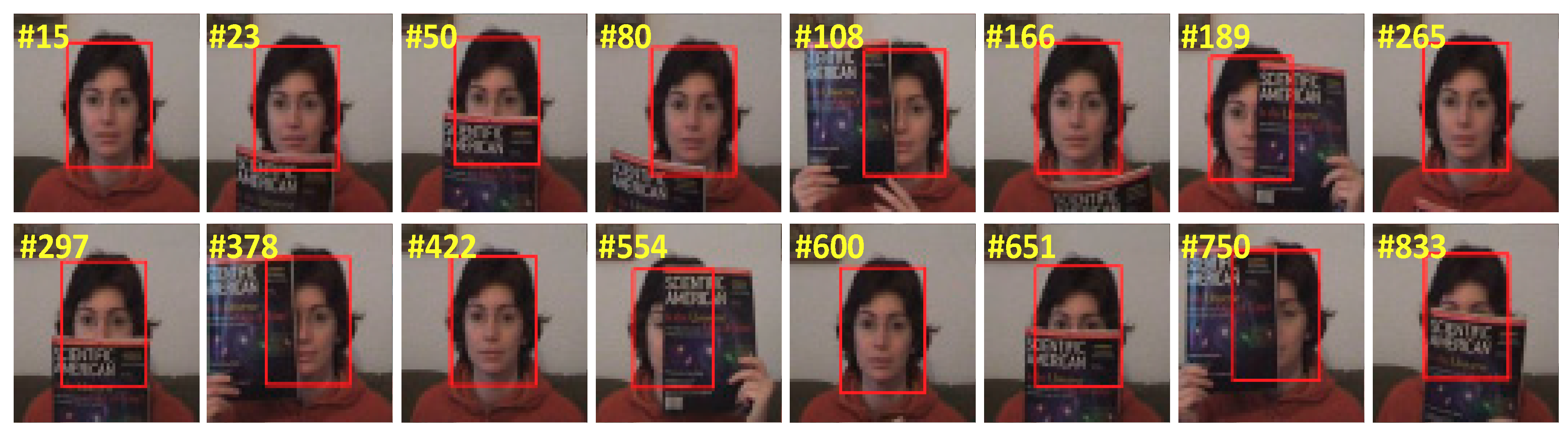
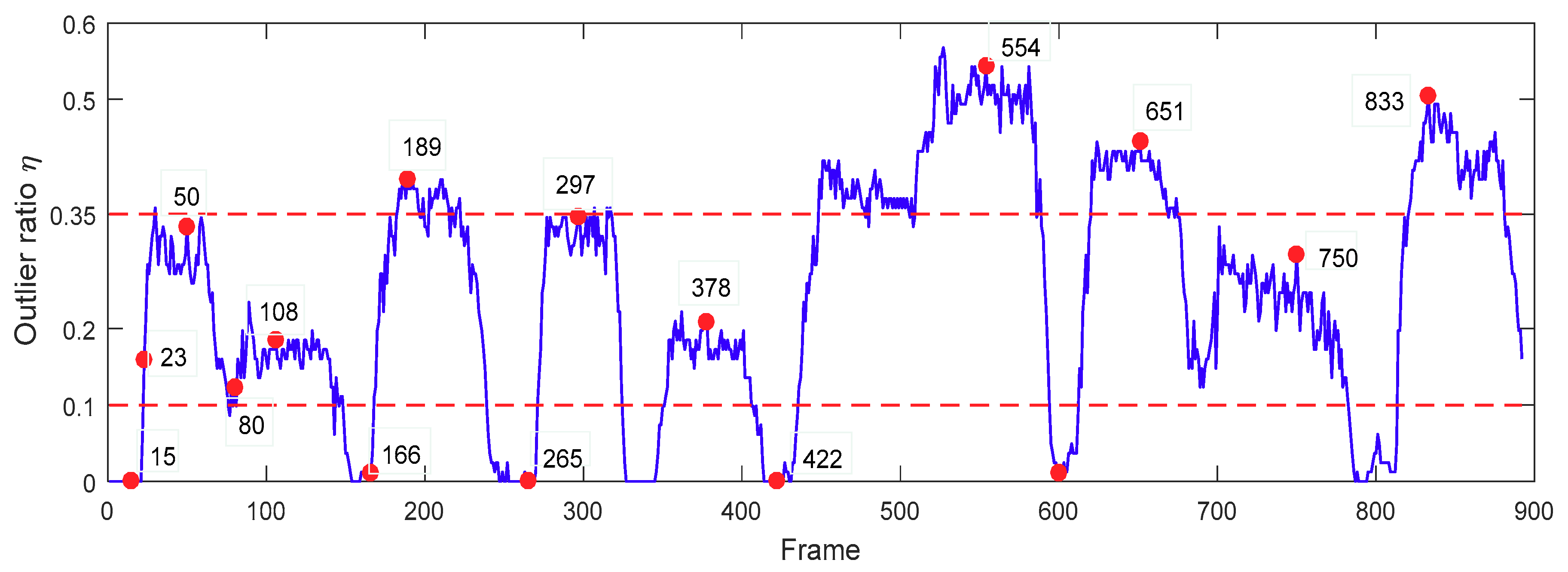
The values of two thresholds tr1 and tr2 were determined experimentally. An illustration of the variation of the outlier ratio $\mathsf{\eta }$ is shown in Figure 3. We could see that the values of $\eta$ were smaller than 0.1 in the absence of occlusion (e.g., #15, #166, #265, #422, #600), which meant that the object was normal. When the object was heavily occluded, the values of $\eta$ were larger than 0.35 (e.g., #189, #554, # 651, #833), which indicated serious outlier. Therefore, we set the threshold tr1 = 0.1, and tr2 = 0.35.

6. Experiments

6.1. Experiment Settings

The proposed tracker was implemented in MATLAB R2017a on a PC with Intel i5-7400 CPU (3.0 GHz) and 16 GB memory. We evaluated the tracking performance on the OTB-2013 benchmark dataset [26] that contains 51 challenging sequences.

The parameters of our tracker for all test sequences were fixed to demonstrate its robustness and stability. The target region division was shown in Section 3.1. The number of target templates n was set to 10. We manually labeled the location of the target in the first frame for each sequence and set K = 40, λ = 0.01 and γ = 0.01. The number of particles was 600 and the variance matrix of affine parameters was set as Σ = diag (4, 4, 0.01, 0.005). For the template update, ten eigenvectors were used to carry out the incremental subspace learning method every five frames.

To evaluate the performance of the trackers, we adopted three widely used metrics [26]: (i) the center location error (CLE), which computes the average Euclidean distance between the center locations of the tracked targets and the ground truth positions of all the frames; (ii) distance precision, which is calculated as the percentage of tracking frames, where the estimated locations are within a given threshold distance; (iii) the success rate, which is calculated as the percentage of tracking frames where the bounding box overlap rate surpasses a given threshold. The overlap rate is defined by PASCAL VOC criteria [40], score = $\frac{area\left({\mathrm{ROI}}_{\mathrm{T}}\cap {\mathrm{ROI}}_{\mathrm{G}}\right)}{area\left(RO{I}_T\cup RO{I}_G\right)}$, where ${\mathrm{ROI}}_{\mathrm{T}}$ is the tracking bounding box and ${\mathrm{ROI}}_{\mathrm{G}}$ is the ground truth bounding box. $\cap$ and $\cup$ stand for the intersection and union of two regions in pixels, respectively.

6.2. Overall Performance

We compared the proposed tracker with nine other trackers, including VTD [5], L1APG [7], ASLA [9], CSK [18], Frag [27], TLD [35], STC [41], DLT [42], CT [43]. Among them, the ASLA, VTD and Frag are patch-based tracking methods. The CSK and STC are based on CFs. The DLT is based on deep neural networks. The CT is based on the compressive sensing theory. We used the results proposed by the OTB-2013 benchmark or available source codes to reproduce the results. The precision and success plots in terms of one-pass evaluation (OPE) [26] are provided in Figure 4. In the precision plots, we used the distance precision at a threshold of 20 pixels for ranking, while in the success plots, we used the area under curve (AUC) for ranking.

As shown in Figure 4, the precision and success scores of our tracker were 0.580 and 0.463, which were ranked the second and first places, respectively. Compared with the baseline ASLA, our tracker achieved an improvement (4.8% in the precision rate and 2.9% in the success rate). The improvement in performance as compared to the ASLA can be attributed to two aspects: (i) we modeled the appearance of the object by the combination of the patch descriptor and the patch sparse coefficients, which made the tracker more robust to changes of target appearance, because the uses of patch descriptors allowed us to adjust the contribution of each patch in the observation model according to appearance changes; (ii) we designed an outlier-aware template update scheme to alleviate the model drift caused by outlier samples. The VTD and Frag are also the patch-based trackers. Our tracker outperformed the VTD by 4.7% and the Frag by 11.3% in the success plot, respectively. Compared to the CSK and STC, the proposed tracker showed higher precision and success scores. For the deep learning-based tracker, our tracker outperformed the DLT by 4.8% on the success score.

6.3. Attribute-Based Analysis

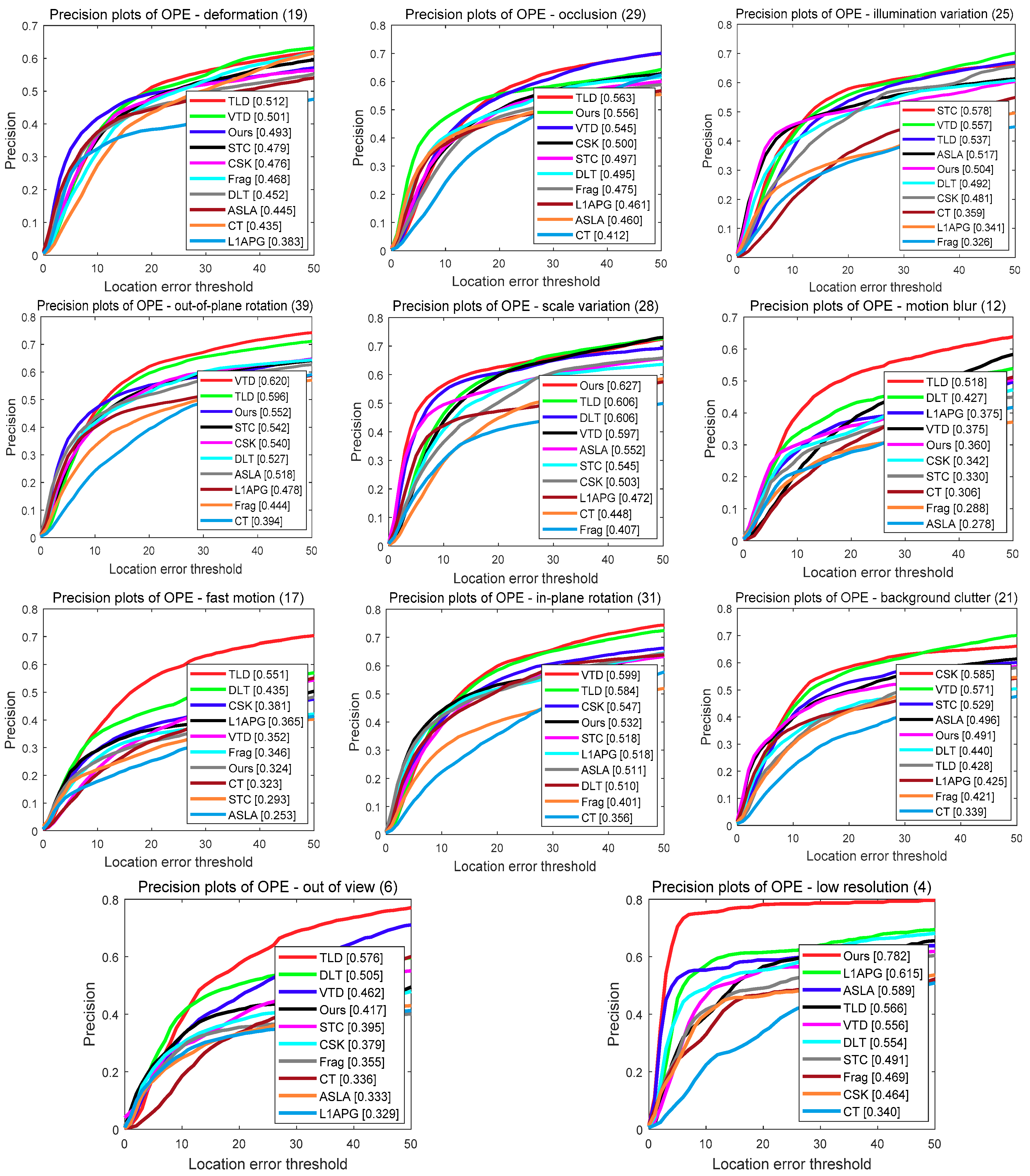
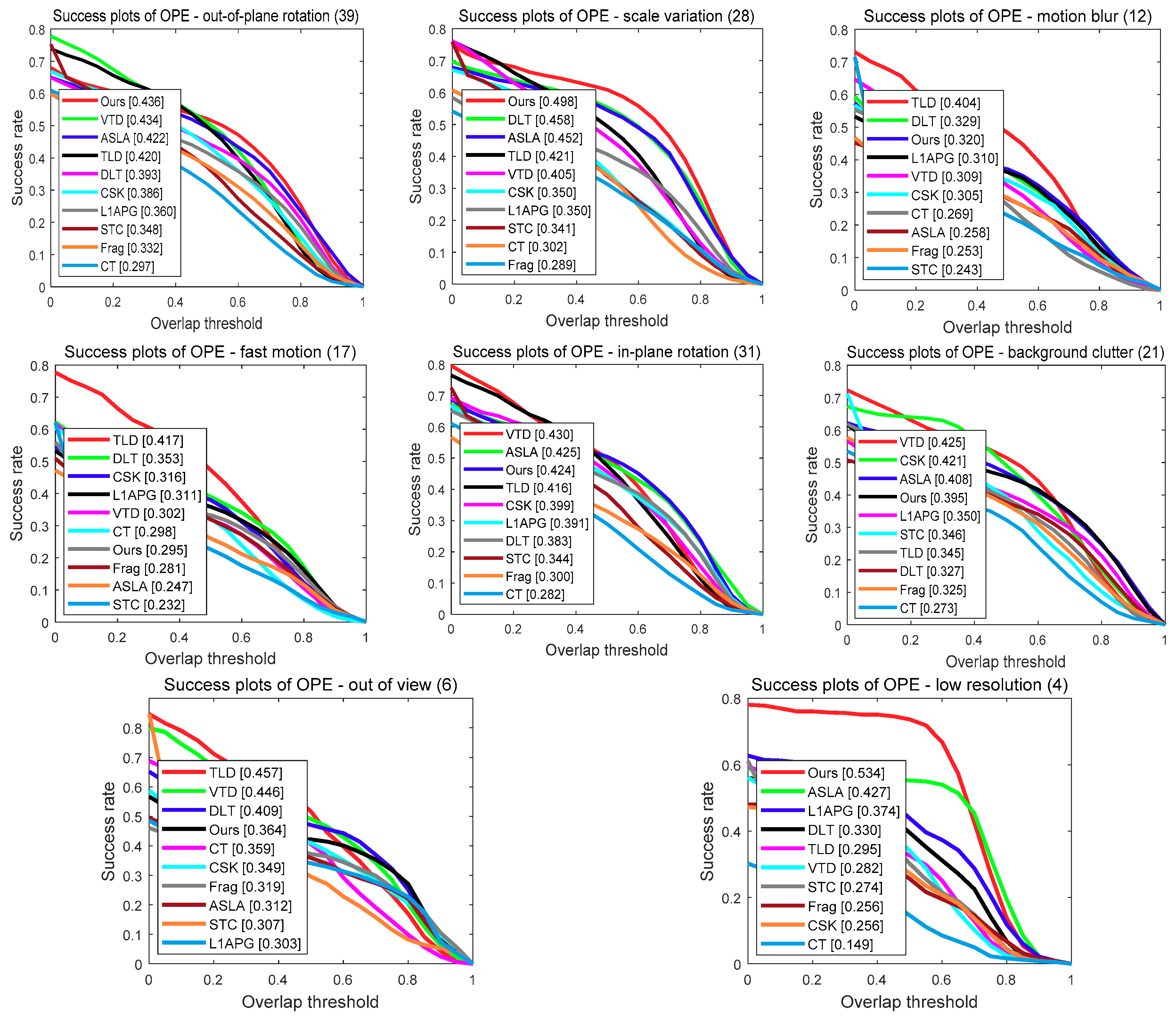
In this subsection, to further evaluate the performance of our tracker under different challenges, we conducted an attribute-based evaluation on the OTB-2013 benchmark dataset. The dataset video sequences were annotated with 11 attributes including occlusion, illumination variation, scale variation, fast motion, motion blur, deformation, background clutters, out-of-view, out-of-plane rotation, in-plane rotation and low resolution. We reported the precision plots and success plots of different trackers on these 11 attributes in Figure 5, respectively.

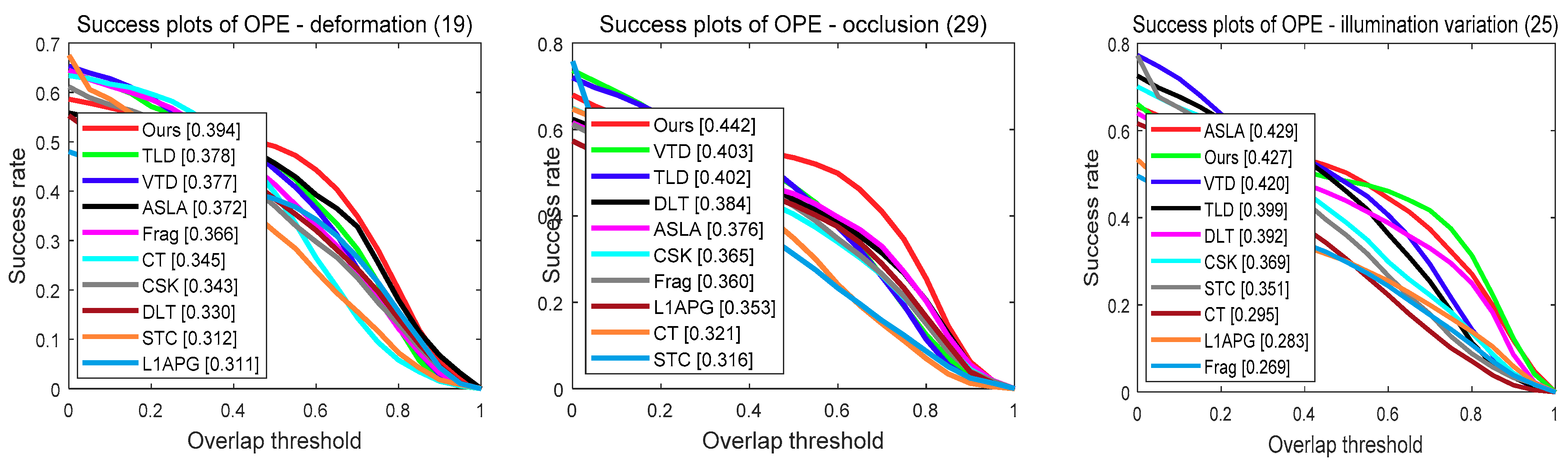
In the precision plots, as shown in Figure 5, our tracker outperformed the baseline ASLA on 9 of 11 attributes. Specially, in the “occlusion”, “motion blur” and “scale variation” attributes, our tracker achieved 9.6%, 8.2% and 7.5% better performance than the ASLA, respectively. Moreover, in terms of success plots, as shown in Figure 6, our tracker also improved the baseline ASLA on 8 attributes. In addition, in the attributes of “deformation”, ”occlusion”, “out-of-plane rotation”, “scale variation” and “low resolution” attributes, our tracker had the best performance among all the evaluation trackers in terms of the success score.

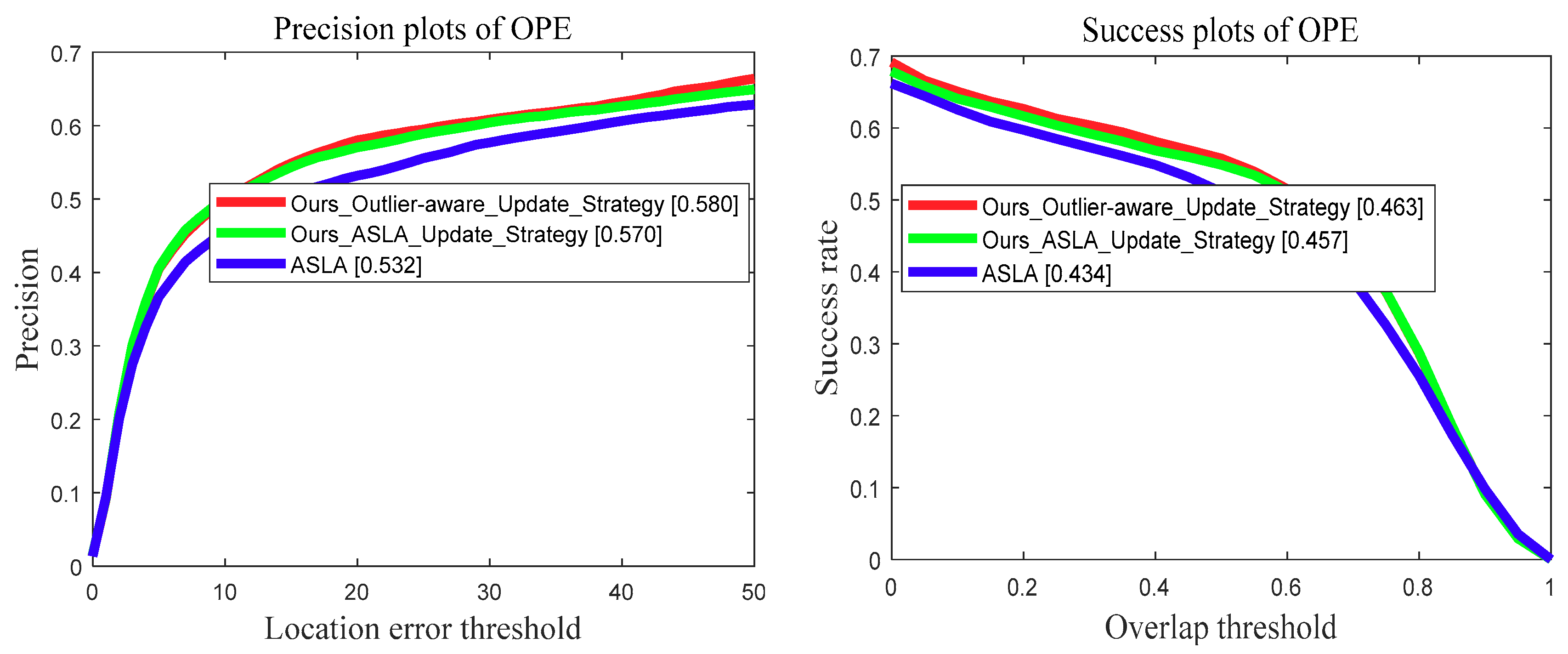
6.4. Evaluation of Template Update Strategy

We further evaluated the proposed outlier-aware template update strategy with comparison to the original template update strategy used in the ASLA [9]. Experimental results on the OTB-2013 benchmark dataset are presented in Figure 7. The “Ours_Outlier-aware_Update_Strategy” denotes our tracker using the proposed outlier-aware template update strategy, and the “Our_ASLA_Update_Strategy” denotes our tracker using the template update strategy proposed in ASLA. Our baseline tracker was the ASLA.

As shown in Figure 7, the proposed outlier-aware template update strategy improved the tracking performance compared to the template update strategy proposed in the ASLA. That was attributed to the added outlier detect module, which alleviated the problem where outlier samples are inadvertently included by the straightforward template update method in the ASLA.

6.5. Typical Results Analysis

We provided more detailed analysis on 12 representative sequences selected from the OTB-2013 benchmark dataset.

Table 1. Average center error (in pixels). The best two results are shown in bold red and blue fonts.

	VTD	Frag	TLD	L1APG	STC	CSK	DLT	CT	ASLA	Ours
Singer1	4.19	88.87	8.00	53.35	5.76	14.01	3.04	15.53	3.29	2.98
David	11.59	82.07	5.12	13.95	12.16	17.69	66.20	10.49	5.07	4.36
Freeman3	23.96	40.47	29.33	33.13	39.44	53.90	4.00	65.32	3.17	2.06
CarScale	38.45	19.74	22.60	79.77	89.35	83.01	22.65	25.95	24.64	14.11
Dudek	10.30	82.69	18.05	23.46	25.60	13.39	8.81	26.53	15.26	11.82
Crossing	26.13	38.59	24.34	63.43	34.07	8.95	1.65	3.56	1.85	1.54
Walking2	46.24	57.53	44.56	5.06	13.83	17.93	2.18	58.53	37.42	1.95
Freeman4	61.68	72.27	39.18	22.12	45.61	78.87	48.09	132.59	70.24	4.57
David3	66.72	13.55	208.00	90.00	6.34	56.10	55.87	88.66	87.76	6.39
FaceOcc1	20.20	10.97	27.37	17.33	250.40	11.93	22.72	25.82	78.06	13.58
Skating1	9.34	149.35	145.45	158.70	66.41	7.79	52.38	150.44	59.86	15.47
Football	13.64	5.36	14.26	15.11	16.13	16.19	191.4	11.91	15.00	4.13
Average	27.70	55.12	48.86	47.95	50.43	31.65	39.92	51.23	33.47	6.91

and

Table 2. Average overlap rate. The best two results are shown in bold red and blue fonts.

	VTD	Frag	TLD	L1APG	STC	CSK	DLT	CT	ASLA	Ours
Singer1	0.49	0.21	0.73	0.29	0.53	0.36	0.85	0.35	0.79	0.86
David	0.56	0.17	0.72	0.54	0.52	0.40	0.25	0.50	0.75	0.76
Freeman3	0.30	0.32	0.45	0.35	0.25	0.30	0.70	0.002	0.75	0.75
CarScale	0.43	0.43	0.45	0.50	0.45	0.42	0.62	0.43	0.61	0.65
Dudek	0.80	0.54	0.65	0.69	0.59	0.72	0.79	0.65	0.74	0.78
Crossing	0.32	0.31	0.40	0.21	0.25	0.48	0.72	0.68	0.79	0.78
Walking2	0.33	0.27	0.31	0.76	0.52	0.46	0.82	0.27	0.37	0.81
Freeman4	0.16	0.14	0.34	0.35	0.16	0.13	0.14	0.005	0.13	0.61
David3	0.40	0.67	0.10	0.38	0.43	0.50	0.46	0.31	0.43	0.71
FaceOcc1	0.68	0.82	0.59	0.75	0.19	0.80	0.59	0.64	0.32	0.79
Skating1	0.53	0.13	0.19	0.10	0.35	0.50	0.43	0.09	0.50	0.52
Football	0.56	0.70	0.49	0.55	0.51	0.55	0.23	0.61	0.53	0.71
Average	0.46	0.39	0.45	0.46	0.40	0.47	0.55	0.38	0.56	0.73

report the comparison results of our tracker and 9 other trackers in terms of the average center location error and average overlap rate. More accurate trackers had lower center location errors and higher overlap rates. Through the results of the tables, we can see that our tracking method obtained smaller center location errors and higher overlap rates on these challenging sequences.

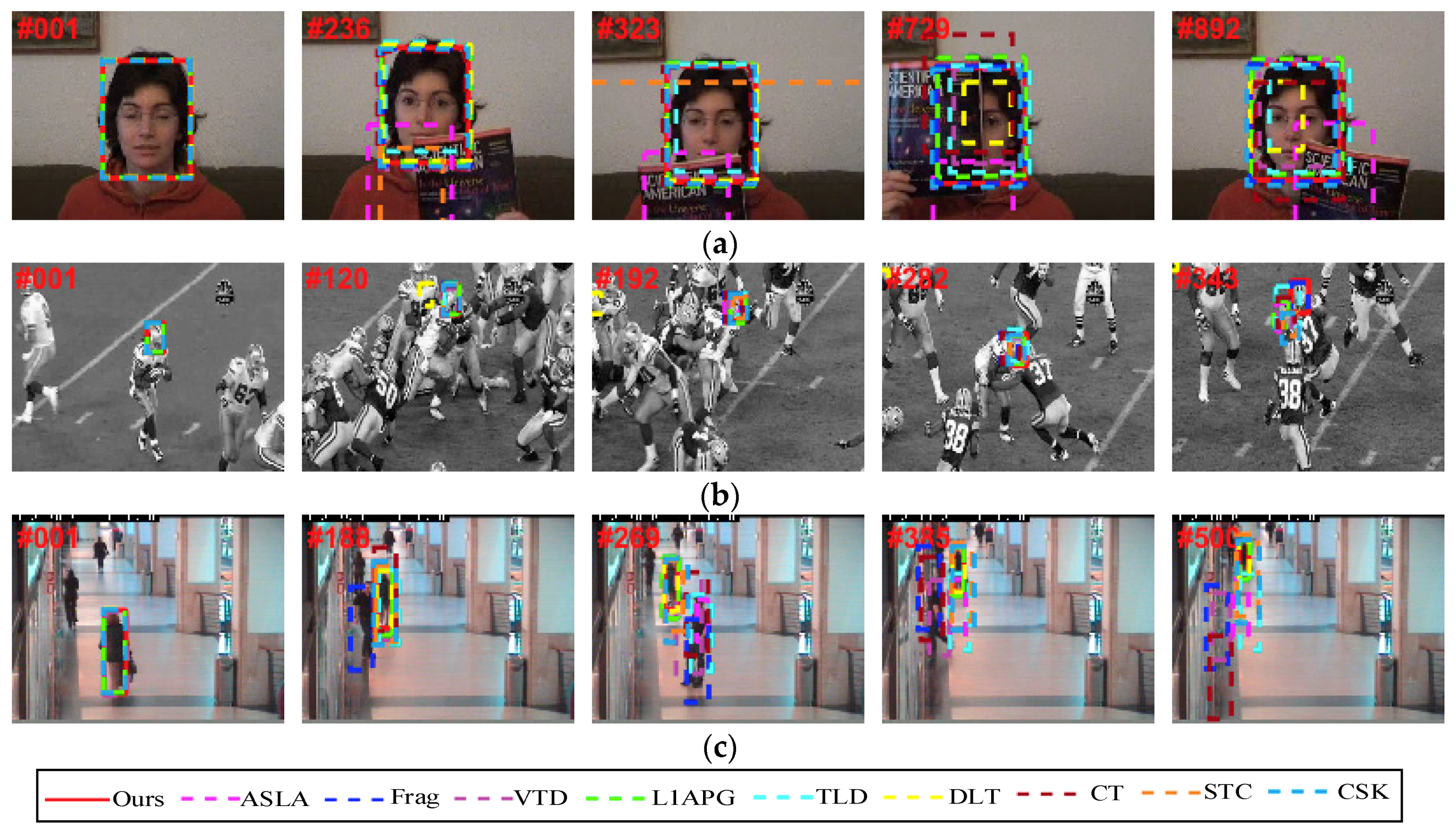
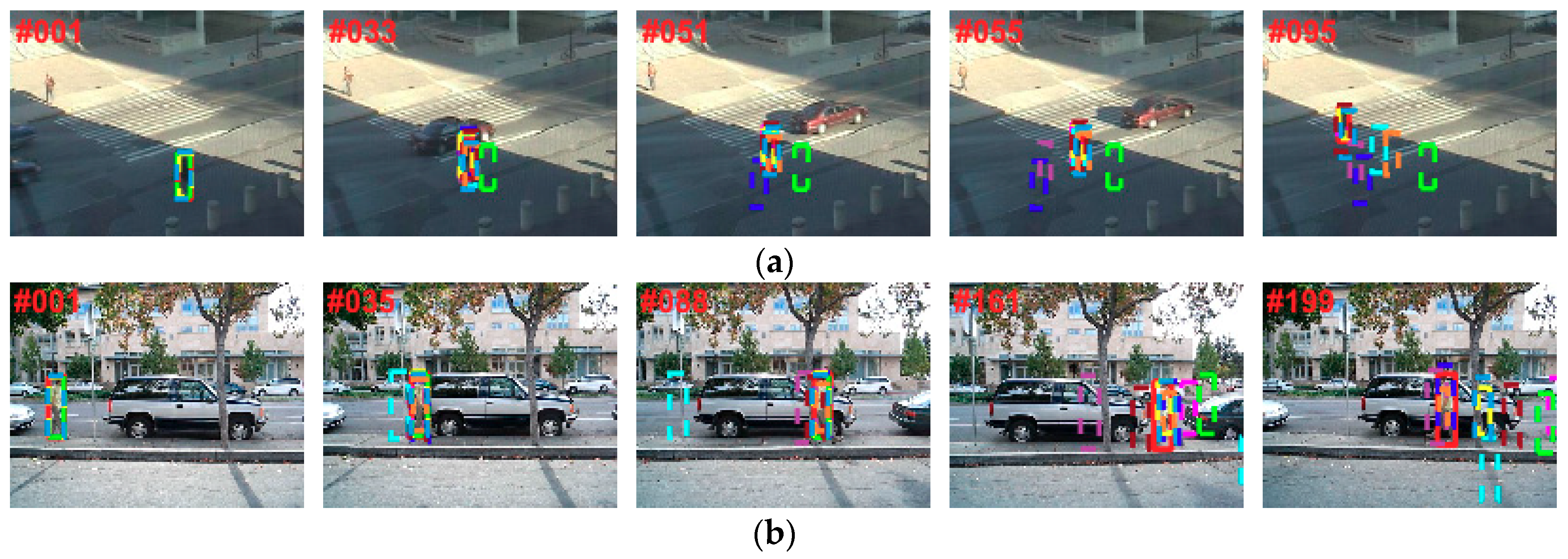
Figure 8, Figure 9, Figure 10 and Figure 11 show some screenshots of the tracking results, marked by different colorful bounding boxes. For these sequences, several principal factors that have effects on the appearance of an object were considered. Some other factors were also included in the discussion.

Occlusion: The sequences FaceOcc1, Football and Walking2 were chosen to demonstrate the effect of partial occlusion. In the FaceOcc1 sequence, all trackers except the STC and ASLA could track the object properly, and the ASLA lost the object when the face occlusion happened, as shown in Figure 8a. The Football sequence (Figure 8b) contained occlusion and background clutters. When the tracked object came into the dense group of players (e.g., #120 and #192), the DLT lost the object. For the surveillance video Walking2 (Figure 8c), the walking woman was occluded by a man over a long time. The Frag, VTD, TLD and CT lost the object when occlusion occurred (e.g., #269 and #385). The STC and CSK did not scale well when the scale of object changed. Only the L1APG, DLT and our method could accurately track the object till the end.

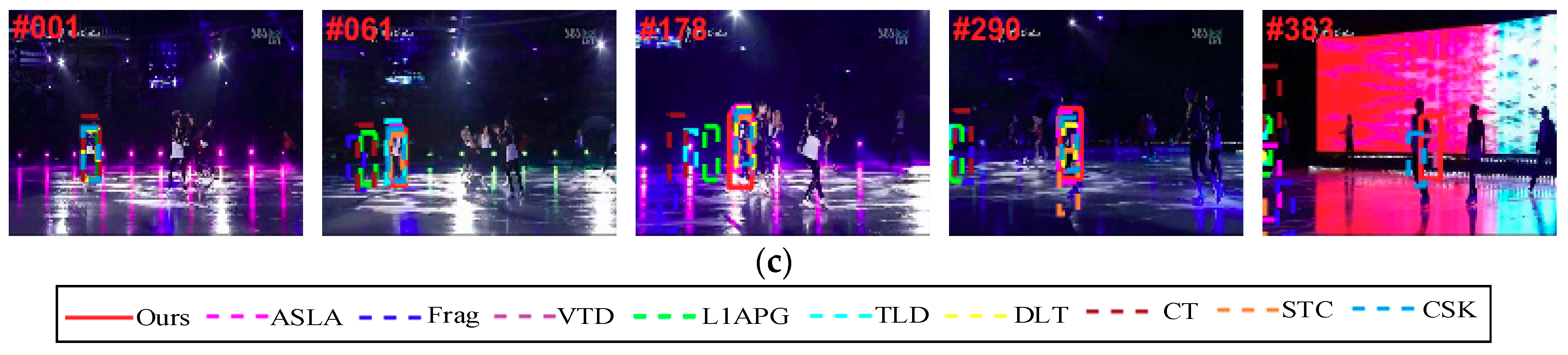
Deformation:Figure 9 presents some sampled results in three sequences where objects underwent deformations. In the Crossing sequence (Figure 9a), the walking person moved from a shadow area to a bright one. Nonrigid deformation and drastic illumination variation were the main challenges. The VTD, Frag, TLD, L1APG and STC lost the object in the tracking process (e.g., #55 and #95). For the David3 sequence (Figure 9b), occlusion was introduced by tree (e.g., #88) and object appearance changed drastically when the man turned around (e.g., #161). Only the Frag, STC and our tracker successfully located the correct object throughout the sequence. The object in the Skating1 sequence (Figure 9c) suffered from frequent non-rigid appearance changes and illumination variations. The Frag, CT and L1APG lost the object around frame 61, but the VTD and our tracker could survive to the end.

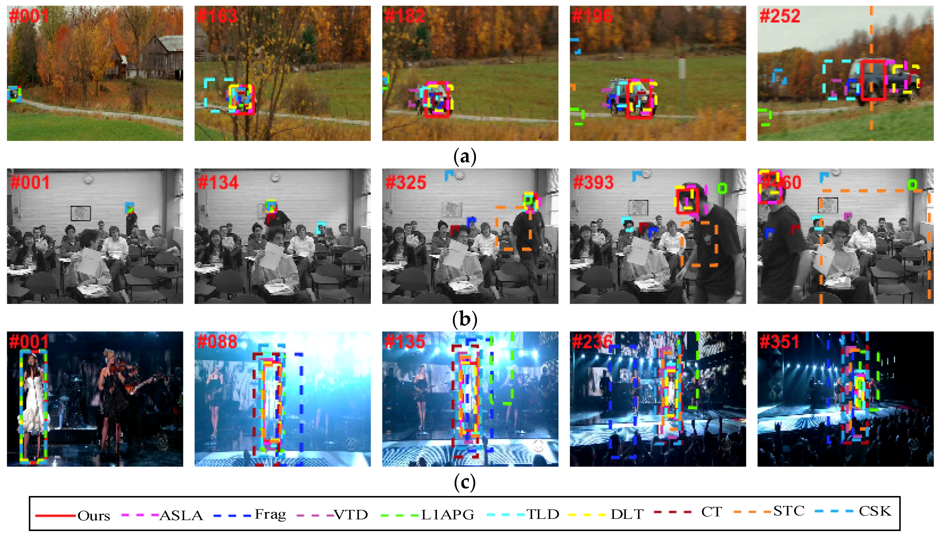
Scale variation:Figure 10 shows screenshots of three videos in which the objects underwent scale variations. For the CarScale sequence (Figure 10a), we can see that the TLD, VTD, L1APG, CSK and STC failed to locate the car when it moved closer to the camera. In the Freeman3 sequence (Figure 10b), the scale of the man changed largely. Only the DLT, ASLA and our tracker could reliably track the object at the most frames. Figure 10c shows the tracking results in the Singer1 sequence, where significant scale and illumination variation were noticed. The Frag and L1APG could not adapt to the scale variation and finally failed to track the object at different time instances (e.g., #88 and #135), and the CT and CSK obtained wrong size of the object (e.g., #236 and # 351).

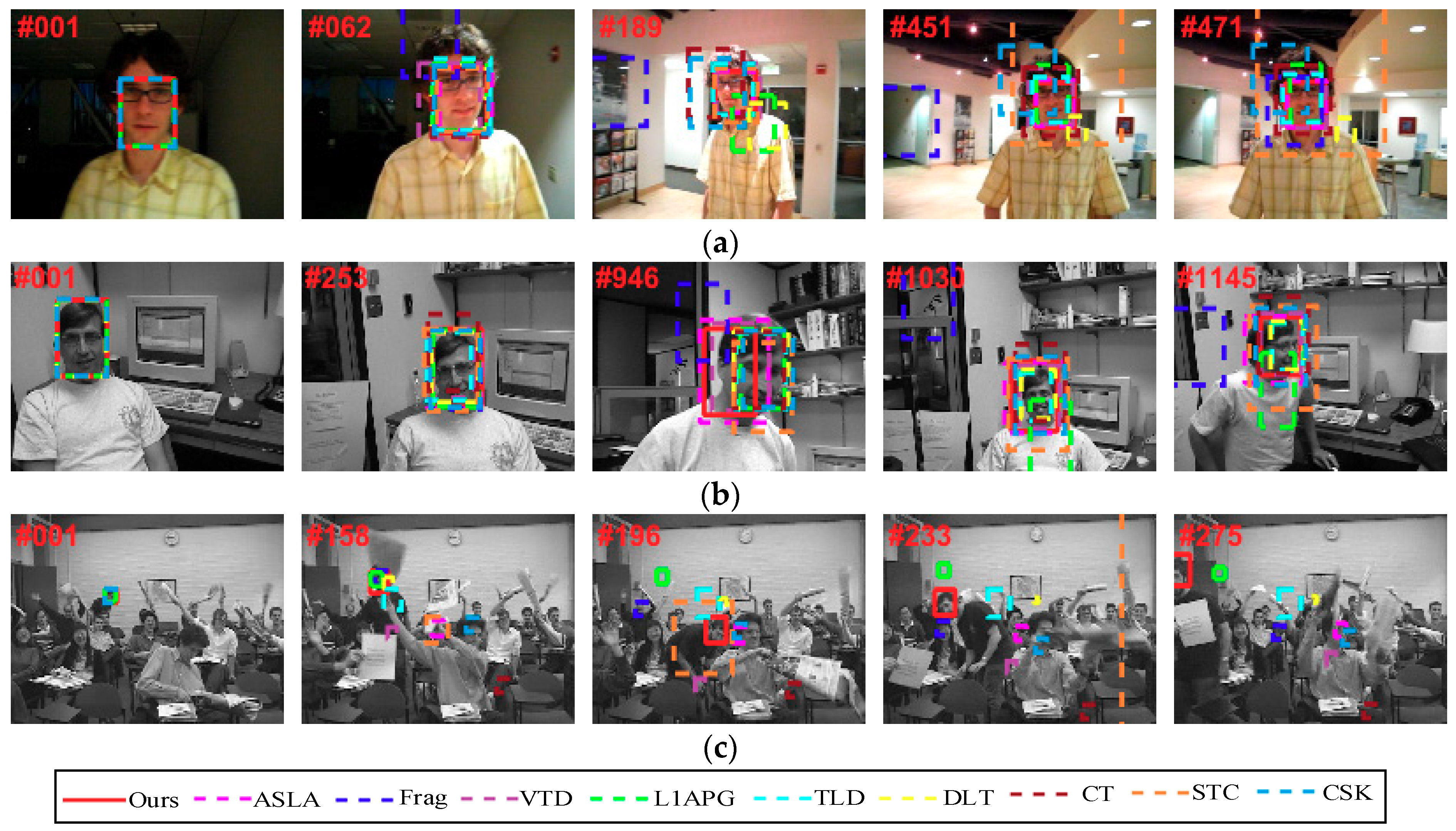
Rotation: In the David sequence (Figure 11a), the person changed the orientation of his face over time, and the varying illumination also made the tracking harder. The Frag and DLT failed to locate the object (e.g., #62 and #189). For the Dudek sequence (Figure 11b), the pose of the man varied slightly. The Frag lose the object (e.g., # 946 and #1030). The Freeman4 sequence (Figure 11c) included rotation and occlusion. It was difficult to handle both of these two challenges. Only our tracker could track the object well.

7. Conclusions

In this paper, we presented a tracking method utilizing the patch descriptor and the structural local sparse representation. The novelty of the paper is to design the patch descriptors defined as the proportion of sub-patches, of which the reconstruction error was less than the given threshold, which would distinguish each patch of the target candidate and reflect the degree of corruption or occlusion of the target. In order to effectively reduce model drift caused by noisy updates, we designed an outlier ratio to describe the outlier degree of a target object. When the outlier ratio was larger than the threshold, we stopped updating the template. Both the quantitative and qualitative evaluations on the OTB-2013 benchmark dataset have been done to verify the effectiveness of the proposed algorithm.

References

- Krafka, K.; Khosla, A.; Kellnhofer, P.; Kannan, H. Eye Tracking for Everyone. In Proceedings of the IEEE Conference on Computer Vision and Pattern Recognition (CVPR), Las Vegas, NV, USA, 26 June–1 July 2016; pp. 2176–2184. [Google Scholar]
- Bharati, S.P.; Wu, Y.; Sui, Y.; Padgett, C.; Wang, H. Real-Time Obstacle Detection and Tracking for Sense-and-Avoid Mechanism in UAVs. IEEE Trans. Intell. Veh. 2018, 3, 185–197. [Google Scholar] [CrossRef]
- Zheng, F.; Shao, L.; Han, J. Robust and Long-Term Object Tracking with an Application to Vehicles. IEEE Trans. Intell. Transp. Syst. 2018. [Google Scholar] [CrossRef]
- Ross, D.A.; Lim, J.; Lin, R.S.; Yang, M.H. Incremental Learning for Robust Visual Tracking. Int. J. Comput. Vis. 2008, 77, 125–141. [Google Scholar] [CrossRef]
- Kwon, J.; Lee, K.M. Visual Tracking Decomposition. In Proceedings of the IEEE Conference on Computer Vision and Pattern Recognition (CVPR), San Francisco, CA, USA, 13–18 June 2010; pp. 1269–1276. [Google Scholar]
- Wright, J.; Yang, A.Y.; Ganesh, A.; Sastry, S.S.; Ma, Y. Robust Face Recognition via Sparse Representation. IEEE Trans. Pattern Anal. Mach. Intell. 2009, 31, 210–227. [Google Scholar] [CrossRef] [PubMed] [Green Version]
- Mei, X.; Ling, H.B. Robust Visual Tracking using L1 Minimization. In Proceedings of the International Conference on Computer Vision (ICCV), Kyoto, Japan, 29 September–2 October 2009; pp. 1436–1443. [Google Scholar]
- Mei, X.; Ling, H.B. Robust Visual Tracking and Vehicle Classification via Sparse Representation. IEEE Trans. Pattern Anal. Mach. Intell. 2011, 33, 2259–2272. [Google Scholar] [PubMed] [Green Version]
- Jia, X.; Lu, H.; Yang, M.H. Visual Tracking via Adaptive Structural Local Sparse Appearance Model. In Proceedings of the IEEE Conference on Computer Vision and Pattern Recognition (CVPR), Providence, RI, USA, 16–21 June 2012; pp. 1822–1829. [Google Scholar]
- Guo, J.; Xu, T.; Shen, Z.; Shi, G. Visual Tracking via Sparse Representation with Reliable Structure Constraint. IEEE Signal Process. Lett. 2017, 24, 146–150. [Google Scholar] [CrossRef]
- Lan, X.; Zhang, S.; Yuen, P.C.; Chellappa, R. Learning Common and Feature-specific Patterns: A Novel Multiple-sparse-representation-based Tracker. IEEE Trans. Image Process. 2018, 27, 2022–2037. [Google Scholar] [CrossRef] [PubMed]
- Zhang, C.; Li, Z.; Wang, Z. Joint Compressive Representation for Multi-Feature Tracking. Neurocomputing 2018, 299, 32–41. [Google Scholar] [CrossRef]
- Avidan, S. Ensemble Tracking. IEEE Trans. Pattern Anal. Mach. Intell. 2007, 29, 261–271. [Google Scholar] [CrossRef] [PubMed]
- Grabner, H.; Leistner, C.; Bischof, H. Semi-supervised On-line Boosting for Robust Tracking. In Proceedings of the European Conference on Computer Vision (ECCV), Marseille, France, 12–18 October 2008; pp. 234–247. [Google Scholar]
- Babenko, B.; Yang, M.H.; Belongie, S. Visual Tracking with Online Multiple Instance Learning. In Proceedings of the IEEE Conference on Computer Vision and Pattern Recognition (CVPR), Miami, FL, USA, 20–25 June 2009; pp. 983–990. [Google Scholar]
- Hare, S.; Saffari, A.; Torr, P.H.S. Struck: Structured Output Tracking with Kernels. In Proceedings of the International Conference on Computer Vision (ICCV), Barcelona, Spain, 6–13 November 2011; pp. 263–270. [Google Scholar]
- Bolme, D.S.; Beveridge, J.R.; Draper, B.A.; Lui, Y.M. Visual Object Tracking using Adaptive Correlation Filters. In Proceedings of the IEEE Conference on Computer Vision and Pattern Recognition (CVPR), San Francisco, CA, USA, 13–18 June 2010; pp. 2544–2550. [Google Scholar]
- Henriques, J.F.; Caseiro, R.; Martins, P.; Batista, J. Exploiting the Circulant Structure of Tracking-by-detection with Kernels. In Proceedings of the European Conference on Computer Vision (ECCV), Florence, Italy, 7–13 October 2012; pp. 702–715. [Google Scholar]
- Henriques, J.F.; Caseiro, R.; Martins, P.; Batista, J. High-Speed Tracking with Kernelized Correlation Filters. IEEE Trans. Pattern Anal. Mach. Intell. 2015, 37, 583–596. [Google Scholar] [CrossRef] [PubMed] [Green Version]
- Danelljan, M.; Häger, G.; Khan, F.S.; Felsberg, M. Accurate Scale Estimation for Robust Visual Tracking. In Proceedings of the British Machine Vision Conference (BMVC), Nottingham, UK, 1–5 September 2014; pp. 65.1–65.11. [Google Scholar]
- Bertinetto, L.; Valmadre, J.; Golodetz, S.; Miksik, O.; Torr, P.H.S. Staple: Complementary Learners for Real-Time Tracking. In Proceedings of the IEEE Conference on Computer Vision and Pattern Recognition (CVPR), Las Vegas, NV, USA, 26 June–1 July 2016; pp. 1401–1409. [Google Scholar]
- Ma, C.; Huang, J.B.; Yang, X.; Yang, M.H. Hierarchical Convolutional Features for Visual Tracking. In Proceedings of the International Conference on Computer Vision (ICCV), Santiago, Chile, 13–16 December 2015; pp. 3074–3082. [Google Scholar]
- Qi, Y.; Zhang, S.; Qin, L.; Yao, H.; Huang, Q.; Lim, J.; Yang, M.H. Hedged Deep Tracking. In Proceedings of the IEEE Conference on Computer Vision and Pattern Recognition (CVPR), Las Vegas, NV, USA, 26 June–1 July 2016; pp. 4303–4311. [Google Scholar]
- Danelljan, M.; Bhat, G.; Khan, F.S.; Felsberg, M. ECO: Efficient Convolution Operators for Tracking. In Proceedings of the IEEE Conference on Computer Vision and Pattern Recognition (CVPR), Honolulu, HI, USA, 21–26 July 2017; pp. 6638–6646. [Google Scholar]
- Li, X.; Hu, W.; Shen, C.; Zhang, Z.; Dick, A.; Hengel, A.V.D. A Survey of Appearance Models in Visual Object Tracking. ACM Trans. Intell. Syst. Technol. 2013, 4, 58:1–58:48. [Google Scholar] [CrossRef]
- Wu, Y.; Lim, J.; Yang, M.H. Online Object Tracking: A Benchmark. In Proceedings of the IEEE Conference on Computer Vision and Pattern Recognition (CVPR), Portland, OR, USA, 23–28 June 2013; pp. 2411–2418. [Google Scholar]
- Adam, A.; Rivlin, E.; Shimshoni, I. Robust Fragments-based Tracking using the Integral Histogram. In Proceedings of the IEEE Conference on Computer Vision and Pattern Recognition (CVPR), New York, NY, USA, 17–22 June 2006; pp. 798–805. [Google Scholar]
- Kwon, J.; Lee, K.M. Tracking of a Non-Rigid Object via Patch-based Dynamic Appearance Modeling and Adaptive Basin Hopping Monte Carlo Sampling. In Proceedings of the IEEE Conference on Computer Vision and Pattern Recognition (CVPR), Miami, FL, USA, 20–25 June 2009; pp. 1208–1215. [Google Scholar]
- Zhang, T.; Jia, K.; Xu, C.; Ma, Y.; Ahuja, N. Partial Occlusion Handling for Visual Tracking via Robust Part Matching. In Proceedings of the IEEE Conference on Computer Vision and Pattern Recognition (CVPR), Columbus, OH, USA, 24–27 June 2014; pp. 1258–1265. [Google Scholar]
- Cai, Z.; Wen, L.; Lei, Z.; Vasconcelos, N.; Li, S.Z. Robust Deformable and Occluded Object Tracking with Dynamic Graph. IEEE Trans. Image Process. 2014, 23, 5497–5509. [Google Scholar] [CrossRef] [PubMed]
- Wang, X.; Valstar, M.; Martinez, B.; Khan, M.H. TRIC-track: Tracking by Regression with Incrementally Learned Cascades. In Proceedings of the International Conference on Computer Vision (ICCV), Santiago, Chile, 13–16 December 2015; pp. 4337–4345. [Google Scholar]
- Sun, C.; Wang, D.; Lu, H. Occlusion-Aware Fragment-Based Tracking with Spatial-Temporal Consistency. IEEE Trans. Image Process. 2016, 8, 3814–3825. [Google Scholar] [CrossRef] [PubMed]
- Li, Y.; Zhu, J.; Hoi, S.C.H. Reliable Patch Trackers: Robust Visual Tracking by Exploiting Reliable Patches. In Proceedings of the IEEE Conference on Computer Vision and Pattern Recognition (CVPR), Boston, MA, USA, 7–12 June 2015; pp. 353–361. [Google Scholar]
- Chen, W.; Zhang, K.; Liu, Q. Robust Visual Tracking via Patch Based Kernel Correlation Filters with Adaptive Multiple Feature Ensemble. Neurocomputing 2016, 214, 607–617. [Google Scholar] [CrossRef]
- Kalal, Z.; Mikolajczyk, K.; Matas, J. Tracking-Learning-Detection. IEEE Trans. Pattern Anal. Mach. Intell. 2012, 34, 1409–1422. [Google Scholar] [CrossRef] [PubMed] [Green Version]
- Zhang, J.; Ma, S.; Sclaroff, S. MEEM: Robust Tracking via Multiple Experts Using Entropy Minimization. In Proceedings of the European Conference on Computer Vision (ECCV), Zurich, Switzerland, 6–12 September 2014; pp. 188–203. [Google Scholar]
- Ma, C.; Yang, X.; Zhang, C.; Yang, M.H. Long-term Correlation Tracking. In Proceedings of the IEEE Conference on Computer Vision and Pattern Recognition (CVPR), Boston, MA, USA, 7–12 June 2015; pp. 5388–5396. [Google Scholar]
- Danellja, M.; Häger, G.; Khan, F.S.; Felsberg, M. Adaptive Decontamination of the Training Set: A Unified Formulation for Discriminative Visual Tracking. In Proceedings of the IEEE Conference on Computer Vision and Pattern Recognition (CVPR), Las Vegas, NA, USA, 26 June–1 July 2016; pp. 1430–1438. [Google Scholar]
- Shi, R.; Wu, G.; Kang, W.; Wang, Z.; Feng, D.D. Visual Tracking Utilizing Robust Complementary Learner and Adaptive Refiner. Neurocomputing 2017, 260, 367–377. [Google Scholar] [CrossRef]
- Everingham, M.; Gool, L.V.; Williams, C.K.I.; Winn, J.; Zisserman, A. The Pascal Visual Object Classes (VOC) challenge. Int. J. Comput. Vis. 2010, 88, 303–338. [Google Scholar] [CrossRef]
- Zhang, K.; Zhang, L.; Liu, Q.; Zhang, D.; Yang, M.H. Fast Visual Tracking via Dense Spatio-Temporal Context Learning. In Proceedings of the European Conference on Computer Vision (ECCV), Zurich, Switzerland, 6–12 September 2014; pp. 127–141. [Google Scholar]
- Wang, N.; Yeung, D.Y. Learning a Deep Compact Image Representation for Visual Tracking. In Proceedings of the Advances in Neural Information Processing Systems, Stateline, NV, USA, 5–8 December 2013; pp. 809–817. [Google Scholar]
- Zhang, K.; Zhang, L.; Yang, M.H. Real-Time Compressive Tracking. In Proceedings of the European Conference on Computer Vision (ECCV), Florence, Italy, 7–13 October 2012; pp. 864–877. [Google Scholar]
Figure 1.
Target region division. (a) Sampling patches; (b) sampling sub-patches; (c) a patch distribution map.
Figure 2.
Schematic diagram of the proposed tracking method.
Figure 3.
An illustration of the variation of the outlier ratio η on the FaceOcc1 sequence. In the bottom plot, the blue curve reflects the variation of the outlier ratio on each frame, and the two horizontal red dashed lines are the predefined thresholds (set to 0.1 and 0.35 in our approach). We also mark the key frames and their indices with red points in the plot, which are correspondingly shown at the top of the plot.
Figure 4.
The precision and success plots of the tracking results on the OTB-2013 benchmark dataset. The legends contain the scores of the center location error with the threshold of 20 pixels and values of the area under curve for all trackers in the precision and success plots, respectively. Note that the color of one curve is determined by the rank of the corresponding trackers, not their names.
Figure 5.
Precision plots for different attributes. The legend contains the precision score of each tracker at 20 pixels.
Figure 6.
Success plots for different attributes. The legend contains the AUC score of each tracker.
Figure 7.
Evaluation of template update strategy on the OTB-2013 benchmark dataset.
Figure 8.
Screenshots of some sampled tracking results, where objects are heavily occluded. (a) FaceOcc1 with occlusion; (b) Football with occlusion and background clutters; (c) Walking2 with occlusion and scale variation.
Figure 9.
Screenshots of some sampled tracking results, where objects undergo deformations. (a) Crossing with deformation and illumination variation; (b) David3 with deformation and occlusion; (c) Skating1 with deformation and illumination variation.
Figure 10.
Screenshots of some sampled tracking results, where objects suffer from significant scale variations. (a) CarScale with scale variation and occlusion; (b) Freeman3 with scale variation and rotation; (c) Singer1 with scale variation and illumination variation.
Figure 11.
Screenshots of some sampled tracking results, where objects suffer from rotation. (a) David with rotation and illumination variation; (b) Dudek with rotation and scale variation; (c) Freeman4 with rotation and occlusion.