Investigating Feature Selection and Random Forests for Inter-Patient Heartbeat Classification

Abstract

Finding an optimal combination of features and classifier is still an open problem in the development of automatic heartbeat classification systems, especially when applications that involve resource-constrained devices are considered. In this paper, a novel study of the selection of informative features and the use of a random forest classifier while following the recommendations of the Association for the Advancement of Medical Instrumentation (AAMI) and an inter-patient division of datasets is presented. Features were selected using a filter method based on the mutual information ranking criterion on the training set. Results showed that normalized beat-to-beat (R–R) intervals and features relative to the width of the ventricular depolarization waves (QRS complex) are the most discriminative among those considered. The best results achieved on the MIT-BIH Arrhythmia Database were an overall accuracy of 96.14% and F1-scores of 97.97%, 73.06%, and 90.85% in the classification of normal beats, supraventricular ectopic beats, and ventricular ectopic beats, respectively. In comparison with other state-of-the-art approaches tested under similar constraints, this work represents one of the highest performances reported to date while relying on a very small feature vector.

1. Introduction

The electrocardiogram (ECG) is the register of electrical potentials, variable over time, produced by the myocardium during the cardiac cycle. Since its invention at the beginning of the 20th century, the ECG has played a central role in the diagnosis of cardiac arrhythmias and other heart diseases thanks to its simplicity and non-invasive nature. In recent years, thanks to the availability of pocket or wearable devices for single lead ECG recording, it has become possible to perform the acquisition of the ECG signal even in ambulatory contexts for applications of prevention and risk management. The successful application and dissemination of such approaches require the development not only of reliable, but also lightweight algorithms for the automatic detection and classification of signal anomalies in order to reduce the amount of data and the number of events needed to be sent to the physician for making a proper risk assessment and giving advice [1].

In this work, we focus our attention on the problem of classifying single heartbeats and separating the normal electrical activity originated in the sinus node from the ectopic activity originated elsewhere. According to the standard ANSI/AAMI EC57:1998/(R)2008, the methods that perform heartbeat classification should at most distinguish between the following classes: normal beats (NB), supraventricular ectopic beats (SVEB), ventricular ectopic beats (VEB), fusion beats (FB), and unclassifiable or paced beats (UB). Though ectopic beats are generally benign and do not represent any immediate health problem, in prevention and risk management contexts, they become relevant to detect and quantify their frequency. VEB frequency is especially relevant since it can be used as a predictor of the risk of heart failure and death [2]. The risk indication of SVEB is less clear though some researchers have found that their frequency is associated with a greater risk of atrial fibrillation [3].

During the last few decades, the problem of heartbeat classification has been addressed with a plethora of techniques with mixed results. A recent extensive review of heartbeat classification methods is presented by Luz et al. [4]. In the continuous search of better solutions, the exploration in recent years has focused on the implementation of machine learning methods, of which Random Forests (RF) [5] has been one of the most popular approaches. In RF, a group of classifiers is generated in the form of an ensemble (“forest”) of decision trees. The classification of an input sample is determined by the majority classification by the ensemble. RF classifiers can be highly effective [6] and have already been proposed for resource constrained-devices in real-time biomedical applications [7,8,9,10].

One of the first uses of RF for heartbeat classification was reported by Emanet [11] which used the coefficients given by the Discrete Wavelet Transform (DWT) over the ECG signal as features to train the RF classifier. More recently, Alickovic and Subasi [12] also proposed the use of RF with the DWT of the ECG signal but taking a set of different statistical features extracted from the distribution of wavelet coefficients instead of the coefficient themselves. A similar approach that proposes an extensive use of the DWT was also recently proposed by Pan et al. [13]. RF was similarly explored by Ganesh Kumar and Kumaraswamy [14] but with the use of features obtained from the Discrete Cosine Transform (DCT) over the interbeat interval signal. Mahesh et al. [15] used a mix of time-domain features related to the Heart Rate Variability (HRV) and frequency-domain features from the DWT to feed RF. An approach for using RF with a series of time-domain features that includes amplitude differences was proposed by Park et al. [16]. This approach was recently extended to include features resulted from a resampled version of the ECG signal in a cascade configuration of RF classifiers [17].

All of the approaches mentioned have reported accuracies superior to 98% when tested with the MIT-BIH Arrhythmia Database, but few of them follow the recommendations of the AAMI in terms of the type of heartbeat to detect (in particular the classification of SVEB and VEB) and the use of quality measures in addition to overall accuracy (like sensitivity and positive predictivity) which can be distorted by the results of the majority class [4]. Even more importantly, none of the works that have reported the use of RF for heartbeat classification have followed an inter-patient paradigm where the signals used for the training phase are obtained from different patients respect to those used during the test phase. As noted elsewhere [4,18], those limitations make it difficult to make fair comparisons between the different approaches reported in the literature.

In this investigation, we explore the use of RF for performing heartbeat classification while following the AAMI guidelines and the inter-patient paradigm. The study is also focused on the selection of a reduced set of features that allows for optimizing the classification performance without implying a high computational complexity. For this, we consider a feature space composed of several characteristics already found to be relevant in other studies [16,17,18,19,20,21,22,23,24,25,26,27,28] and also introduced some novel considerations for calculating normalized features. An optimal set of features is identified by using a selection approach based on the mutual information (MI) ranking criterion [28]. Results confirm that RF are an excellent tool for heartbeat classification and that few selected features of the ECG are enough to obtain state-of-the-art performance.

2. Materials and Methods

2.1. Datasets

The ECG signals used in this work were obtained from the online repository of the MIT-BIH Arrhythmia Database (http://www.physionet.org/physiobank/database/mitdb). The database included forty-eight 30 min ECG recordings sampled at 360 Hz and collected from two leads. Here, only signals from the modified limb lead II (MLII) are used. Signals were extracted from the original files using the native Python waveform-database (WFDB) package (https://github.com/MIT-LCP/wfdb-python) and resampled at 150 Hz, which is a sampling frequency commonly found in wearables and screening devices. The 109,494 heartbeats present in the MIT-BIH Arrhythmia Database were relabeled from the original 15 heartbeat types into the five types defined by the AAMI (NB, SVEB, VEB, FB, and UB) as described by Luz et al. [4].

Training and testing sets are constructed by following a clinically realistic inter-patient paradigm, where the data used to develop and evaluate the classifier come from different patients. The inter-patient approach implemented here corresponds to the division proposed by de Chazal et al. [29] and adopted by others [4] where the four recordings with paced beats are excluded and the remaining 44 recordings are divided into two datasets each containing 22 recordings. The first set, called DS1, is used for training and is composed of all heartbeats of records: 101, 106, 108, 109, 112, 114, 115, 116, 118, 119, 122, 124, 201, 203, 205, 207, 208, 209, 215, 220, 223, and 230. The second set, called DS2, is used for test and is composed of all heartbeats of records: 100, 103, 105, 11, 113, 117, 121, 123, 200, 202, 210, 212, 213, 214, 219, 221, 222, 228, 231, 232, 233, and 234. The total number of beats on each class using this division is reported in

Table 1. Heartbeat distribution by classes of the different divisions used for constructing the train and test sets. The following classes are considered: normal beats (NB), supraventricular ectopic beats (SVEB), ventricular ectopic beats (VEB), fusion beats (FB), and unclassifiable or paced beats (UB). FB and UB classes were not considered in the classification presented in this work but are nevertheless included in the evaluation.

Dataset	NB	SVEB	VEB	FB	UB	Total
Train (DS1)	45,866	944	3788	415	8	51,021
Test (DS2)	44,259	1837	3221	388	7	49,712

. Due to the low number of FB present in the database as well as the very few UB that remain after excluding paced heartbeats, both types of heartbeats are not considered for classification but are nevertheless included in the evaluation.

The computer code used for dataset preparation as well as feature extraction and selection, and model training and validation is available online (see Supplementary Materials).

2.2. Feature Extraction

A total of 85 features are considered in this study. Most of them have already found to be relevant in other studies including: beat-to-beat (R–R) intervals (used in almost all previous works), discrete wavelet transform (DWT) coefficients [19,20,25], Hermite basis function (HBF) expansion coefficients [21,22,23,24,25], higher order statistics (HOS) [25,26,27], amplitude differences [16,17], Euclidean distances [16,17,25] and temporal characteristics of the ventricular depolarization waves (QRS complex) [19,28]. We also include features resulting from the normalization of R–R intervals, amplitude differences, and QRS temporal characteristics [16,19,28]. Features can be divided into the following groups:

• Heart rate related features (3 features): the current R–R interval ($R{R}_0$) defined by the heartbeat being classified, the previous R–R interval ($R{R}_{-1}$), and the next R–R interval ($R{R}_{+1}$). R–R intervals are calculated from the location of R spikes provided with the database.
• HBF coefficients (15 features): each beat segment, here defined by the samples located 250 ms before and after each R spike, is decomposed using 3, 4, and 5 Hermite functions as described in [21]. The coefficients obtained from fitting Hermite polynomials of degrees 3, 4, and 5 are calculated using the function hermfit provided by the Scikit-Learn package for Python [30].
• HOS (10 features): the third-, and fourth-order cumulant functions (kurtosis and skewness, respectively) for each beat segment are computed. The parameters as defined in [25] are used: the lag parameters range from $-250$ ms to 250 ms centered on the R spike and five equally spaced sample points.
• DWT coefficients (23 features): the DWT of each beat segment is computed using the same parameters defined in [25]: the Daubechies wavelet function (db1) is used with three levels of decomposition.
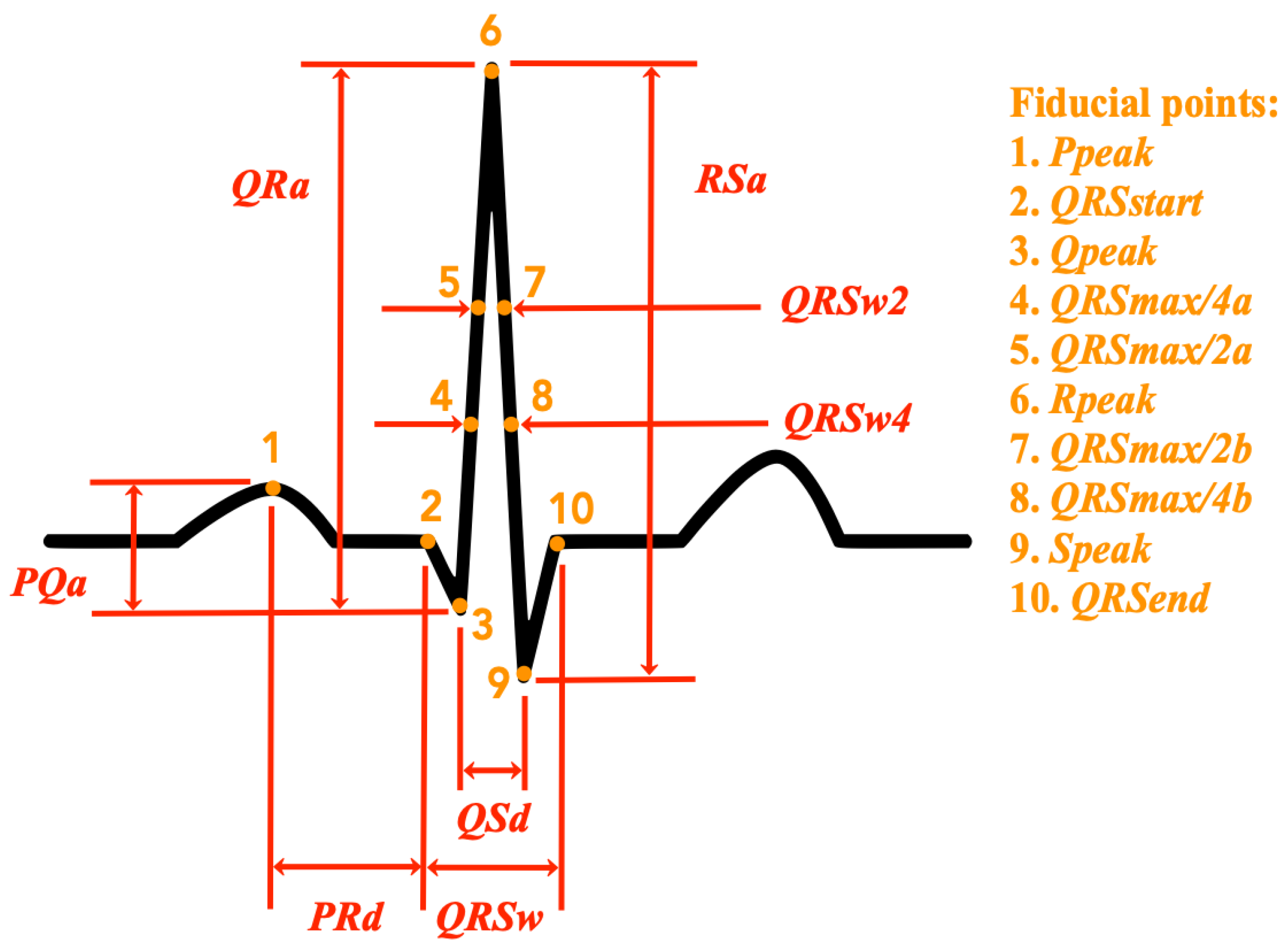
• QRS temporal characteristics (4 features): the following temporal characteristics of the QRS complex are calculated: the total duration of the QRS complex ($QRSw$), the width of the QRS complex at half of the peak value ($QRSw2$), the width of the QRS complex at a quarter of the peak value ($QRSw4$), the distance between the peak of the Q wave, and the peak of the S wave ($QSd$). Figure 1 shows an illustration of these features in relation to the ECG signal of a normal heartbeat. A detailed description of the extraction procedure is provided in Appendix A.
• Amplitude differences (8 features): the following amplitude difference features as defined in [16] are extracted: the amplitude difference between the P and the Q waves ($PQa$), the amplitude difference between the Q and the R waves ($QRa$), the amplitude difference between the R and the S waves ($RSa$), the distance between the peak of the P wave and the beginning of the QRS complex ($PRd$), and the peak value of each of the considered waves ($Ppeak$, $Qpeak$, $Rpeak$, and $Speak$). Figure 1 shows an illustration of these features in relation to the ECG signal of a normal heartbeat. A detailed description of the extraction procedure is provided in Appendix A.
• Euclidean distances (4 features): the Euclidean distance (sample, amplitude) between the R spike peak and four points of the beat segment are obtained as described in [25]. These points correspond to the maximum amplitude value between 250 ms and 139 ms before the R spike, the minimum value between 42 ms and 14 ms before the R spike, the minimum value between 14 ms and 42 ms after the R spike, and maximum value between 139 ms and 250 ms after the R spike.
• Normalized heart rate features (6 features): $R{R}_0$ divided by the average of the last 32 beats ($R{R}_0$/$avgRR$), $R{R}_{-1}$ divided by the average of the last 32 R–R intervals ($R{R}_{-1}$/$avgRR$), $R{R}_{+1}$ divided by the average of the last 32 R–R intervals ($R{R}_{+1}$/$avgRR$), $R{R}_{-1}$ divided by $R{R}_0$ ($R{R}_{-1}$/$R{R}_0$), $R{R}_{+1}$ divided by $R{R}_0$ ($R{R}_{+1}$/$R{R}_0$), and the t-statistic of $R{R}_0$ ($tR{R}_0$) defined by the difference between $R{R}_0$ and $avgRR$ divided by the standard deviation of the last 32 R–R intervals.
• Normalized QRS temporal characteristics and amplitude differences (12 features): the same QRS temporal characteristics and amplitude differences previously specified, except that they are divided by their average value in the last 32 heartbeats.

For the extraction of features, all the records of the datasets are evaluated sequentially one heartbeat after another simulating a real-time scenario. For this reason, normalized features use statistics calculated only from precedent heartbeats instead of statistics over an entire record (patient-wise) as is performed in related works [24,31]. Since only the features related to $R{R}_{+1}$ need a future value, the classification of each heartbeat can be done once the following beat is detected.

2.3. Feature Selection

In order to limit the computational complexity of the solution without compromising the classification performance, the maximum number of features actually considered for the training phase of this study is arbitrarily set to ten. This is in line with expert opinions and previous works which have shown that the number of discriminative features can be very small [19,24,28,32]. For filtering and using only the most informative features relative to the heartbeat type classes, the mutual information (MI) ranking criterion as described by Doquire et al. [28] is followed. The function mutual_info_classif provided by the Scikit-Learn package for Python [30] is used for estimating the MI between each feature and the class labels using the training set DS1.

Table 2. The ten most informative features ranked according to the mutual information criterion [28] relative to the NB, SVEB, and VEB classes.

Rank	Feature
1	$QRSw2$ (normalized)
2	$QRSw4$ (normalized)
3	$R{R}_0$/$avgRR$
4	$R{R}_{+1}$/$R{R}_0$
5	$QRSw2$
6	Fitting coefficient 1 of HBF with degree 4 ($HBFd4c1$)
7	$HBFd4c2$
8	$QRSw4$
9	$HBFd4c0$
10	$R{R}_{-1}$/$R{R}_0$

shows the top ten MI ranked features.

2.4. Classification Performance Measures

In order to assess the performance of our heartbeat classification approach and allow the comparison with other methods found in the literature, the sensitivity ($Se$), positive predictivity ($+P$), F1-score ($F_1$), and overall accuracy ($Acc$) of the classification outcome were calculated. The sensitivity, also found in the literature as recall, refers to the relative number of correct detections of a particular class of heartbeats. The positive predictive value, also called precision, refers to the relative number of true positive heartbeats in all detected heartbeats of that class. The F1-score is the harmonic average of the precision and recall, and here is used to assess the classification performance on each class and compare it with state-of-the-art methods using a single value. The overall accuracy refers to the relative number of correctly classified heartbeats considering all classes. Here, the $Acc$ is used to guide feature selection and model development and as a general indicator of performance. All these performance indicators are calculated from the classification confusion matrix. Performance measures from the training set are calculated with “leave-one-patient-out” cross-validation.

2.5. Heartbeat Classification

The Random Forest (RF) algorithm is the method used in this work for the classification of heartbeats. Briefly, an RF is an ensemble of C trees $T1\left(X\right),T2\left(X\right),...,TC\left(X\right)$, where $X=x1,x2,...,xm$ is an m-dimension vector of inputs. The resulting ensemble produces C outputs $Y1=T1\left(X\right),Y2=T2\left(X\right),...,Yc=Tc\left(X\right)$. $Yc$ is the prediction value by decision tree number c. The output of all these randomly generated trees is aggregated to obtain one final prediction Y, which is the average value of all the trees in the forest. An RF generates C number of decision trees from N number of training samples. For each tree in the forest, bootstrap sampling (i.e., randomly selecting the number of samples with replacement) is performed to create a new training set which is then used to fully grow a decision tree without pruning [33]. In each split of a node of a decision tree, only a small number of m features (input variables) are randomly selected instead of all of them (this is known as random feature selection). This process is repeated to create M decision trees in order to form a randomly generated forest.

The training procedure for a randomly generated forest can be summarized as follows:

• Select a random sample from the training dataset.
• Grow a tree for each random sample with the following modification: at each node, select the best split among a randomly selected subset of input variables, which is the tuning parameter of the random forest algorithm. The tree is fully grown until no further splits are possible and not pruned.
• Repeat steps 1 and 2 until C such trees are grown.

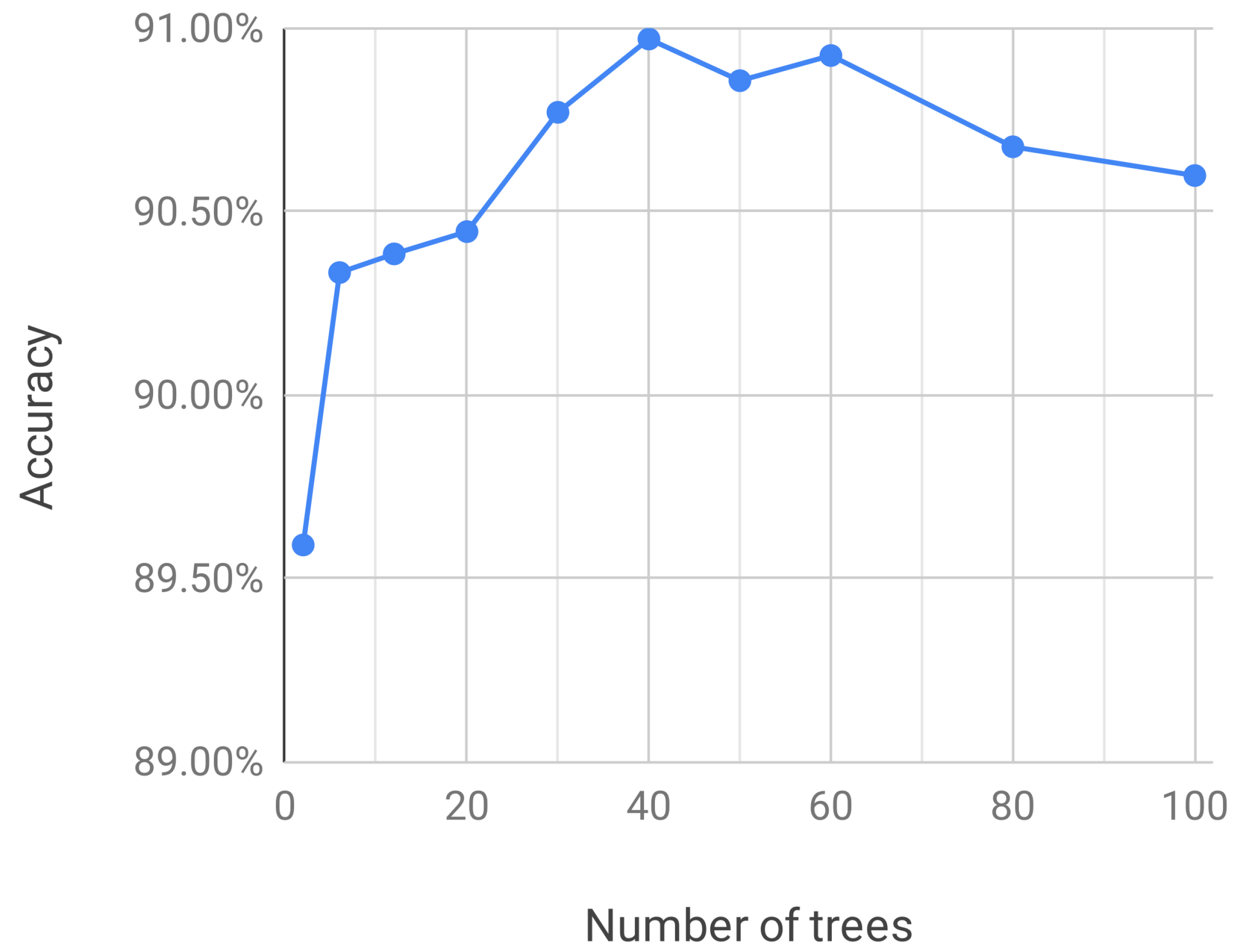
Here, the RF implementation given by the class RandomForestClassifier of the Scikit-learn package for Python [30] is used. The number of trees is the only parameter explored and all other parameters are left with their default values. In order to find an optimum number of trees, classifiers are trained with an increasing number of trees using the top ten features found in the previous section and the performances in terms of $Acc$ are observed. The results obtained from “leave-one-patient-out” cross-validation on the training set DS1 are shown in Figure 2. It can be observed that after 40 trees the performance of classifiers does not increase and may actually diminish.

3. Results

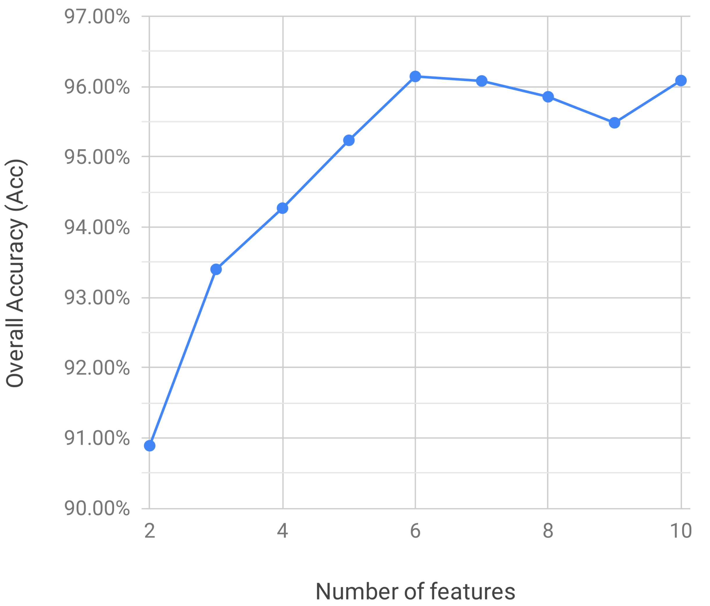
Figure 3 shows the classification performance in terms of $Acc$ on the test set DS2 of RF classifiers that use up to ten MI-ranked features. It can be observed that the highest performance is actually achieved with just six features ($Acc$ = 96.14%) after which the classification performance reaches a plateau.

Table 3. Confusion matrix of obtained on the test set DS2.

		Prediction
		NB	SVEB	VEB
Label	NB	43,494	655	67
	SVEB	369	1443	25
	VEB	383	13	2814
	FB	277	0	65
	QB	4	2	3

shows the confusion matrix obtained with the RF classifier trained with the six most informative features in the test set DS2 and

Table 4. Performance details obtained on the test set DS2.

	$+\mathit{P}$	$\mathit{Se}$	${\mathit{F}}_1$	$\mathit{Acc}$
NB	97.68%	98.27%	97.97%	96.14%
SVEB	68.29%	78.55%	73.06%
VEB	94.62%	87.36%	90.85%

shows the relative performance details.

4. Discussion

In this work, the application of RF for recognizing heartbeats using selected time-domain features extracted from the single-lead ECG signal was investigated following the AAMI guidelines and the inter-patient paradigm. This probably represents the first known attempt to study the performance of RF for heartbeat classification following the AAMI guidelines and the inter-patient paradigm.

In the present investigation, a total of 85 features were explored. We implemented all the features used by Mondéjar-Guerra et al. [25], which is one of the most recent relevant works, and additional morphological features proposed or based on the works of Mar et al. [19] and Doquire et al. [28]. Unlike the feature normalization done by Doquire et al. [28] where normalization is done by dividing values by the patient average (whole record average), in this work, normalization was performed mainly by dividing values by the average of the most recent beats which is an approach that can be more realistically implemented in real-time wearable monitors and screening devices. In order to consider more information about the instantaneous heart rate variation, additional normalizations for R–R intervals were included. In the case of the previous and next R–R interval ($R{R}_{-1}$ and $R{R}_{+1}$), the additional normalization consisted of dividing them by the current R–R interval ($R{R}_0$). This was introduced in an attempt to include the timing relationship between successive R waves as considered in the rules proposed by Tsipouras et al. [34]. In the case of the current R–R interval, the additional normalization was the t-statistic ($tR{R}_0$) which was introduced in order to include a measure of the number of standard deviations a given interval is from the average. Since most of these new normalizations appeared in the top ten most informative features (see Table 2), our results suggest that those newly introduced normalizations for R–R intervals give more information and are more discriminative for heartbeat classification than values of the R–R intervals alone.

Features were selected using the filter approach with mutual information ranking proposed by Doquire et al. [28] and only the top ten most informative ones were considered in the experiments. Results showed that as few as six features were enough to obtain the best performance (see Figure 3). This agrees with the findings of Doquire et al. [28] and de Lannoy et al. [24] which has shown that the number of discriminative features in a set is usually small and that removing the less informative ones can significantly improve the performance of a classifier. In addition to the features based normalized R–R intervals, most of the features among the top ten most informative are relative to the width of the QRS complex peak wave measured at fixed proportions of the peak amplitude. This suggests that those features are probably a more reliable descriptor of QRS morphology than other features based on fiducial points defined by low amplitude changes which can be easily masked by the baseline noise.

Table 5. Comparison of the best results obtained in this work with state-of-the-art approaches.

Work	Classifier	Type of Features	Number of Features Used	${\mathit{F}}_1$ of Class NB	${\mathit{F}}_1$ of Class SVEB	${\mathit{F}}_1$ of Class VEB	$\mathit{Acc}$
Llamedo and Martinez [32]	LD	R–R-intervals, WT, and time domain morphology	8	96.48%	17.16%	83.89%	93%
Huang et al. [31]	Ensemble of SVM + Threshold	R–R-intervals, Random projections	101	97.59%	57.68%	92.37%	93.8%
Afkhami et al. [35]	Ensemble of BDT	R–R-intervals, HOS, GMM	33	97.89%	88.64%	85.82%	96.15%
Chen et al. [37]	SVM	R–R-intervals, DCT Random projections	33	96.88%	33.37%	77.29%	93.1%
Marinho et al. [38]	Naive Bayes	HOS	4	(65.6%) *	(0.4%) *	(84.7%) *	94.0%
Mondéjar- Guerra et al. [25]	Ensemble of SVM	R–R-intervals, HOS, WT, and time domain morphology	45	97.04%	60.74%	94.29%	94.5%
This work	RF	R–R-intervals, HBF and time domain morphology	6	97.97%	73.06%	90.85%	96.14%

WT: wavelet transform, LD: linear discriminant, HOS: high order statistics, HBF: Hermite basis functions, GMM: gaussian mixture model, BDT: bootstrap aggregated decision trees, DCT: discrete cosine transform, SVM: support vector machine. * In [38] $+P$ values nor the confusion matrix are disclosed; therefore, the harmonic mean of the sensitivity and specificity is reported here instead of $F_1$.

shows a comparison between the results obtained with the test set DS2 in this work and some of the approaches with the best heartbeat classification performances following the AAMI guidelines and the inter-patient paradigm reported in the literature. It can be observed that the overall accuracy reported in the present study is one of the highest ever obtained with the same evaluation methodology ($Acc$ = 96.14%), almost the same performance reported by Afkhami et al. [35] ($Acc$ = 96.15%), which is the highest in the literature to the best of our knowledge. Interestingly, though Afkhami et al. propose the use of a different set of features, basically by introducing the use of a Gaussian mixture model (GMM) based on the Expectation Maximization (EM) algorithm, they propose a classification method very similar to RF called Bagging Trees (BT), which is also based on an ensemble of decision trees. RF and BT basically differ in the way the problem of high variance and instability of single decision trees is approached. While BT improves variance by averaging/majority selection of outcome from multiple fully grown trees on variants of training set, RF does the same by random selection of feature-subset for split at each node. Since the RF approach produces a lower correlation between trees, it can potentially produce better results as observed by some studies [36]. The results reported by Afkhami et al. were obtained with an ensemble of 100 trees, whereas the results presented here were obtained with an ensemble of only 40 trees.

Since the highest performance detecting SVEB was reported by Afkhami et al. [35], a possible route for improvement can be to include in our feature selection procedure the GMM-based features proposed by Afkhami et al. However, given the limitations of the MIT-BIH Arrhythmia Database and the inter-patient protocol proposed by de Chazal et al. [29], the performance in the detection of SVEB of the proposed approach as well as many others should not be taken as definitive. For this, more research considering additional databases is needed.

Given that normalized features seem to be very discriminative, another interesting path for future investigation can be to further explore the effect of different types of normalization in the feature ranking and classification performance. In particular, it can be worth exploring to consider a larger number of beats for calculating the averages. As noted before, some previous works implemented record-wise (patient-wise) normalization [24,28,31], but this implies using information of many future beats for classifying any given one which may not be realistically implemented in ambulatory screening and real-time applications. Only past information should be used for those cases. However, if several minutes of previous activity are needed in order to calculate normalized features, the effective number of analyzed beats of current datasets may be substantially reduced.

5. Conclusions

In this study, time-domain features extracted from the single-lead ECG were objectively selected by their information content, and the heartbeat classification performance using RF was fairly evaluated by following the AAMI guidelines and the inter-patient paradigm. Normalized features relative to R–R intervals and to the width of the main wave of the QRS complex were found to be the most discriminative characteristics for the classification task. The best results were obtained with the top six most informative features and a 40-trees RF classifier. The evaluation on the MIT-BIH Arrhythmia Database resulted in an overall accuracy was 96.14% with specific F1-scores of 97.97%, 73.06%, and 90.85% for the NB, SVEB, and VEB classes, respectively. In comparison with state-of-the-art approaches evaluated on similar conditions, our results represent one of the highest performances obtained to date. Results not only confirm that RF are an excellent tool for heartbeat classification but also that relatively few characteristics are enough to obtain state-of-the-art performance.

References

- Scirè, A.; Tropeano, F.; Anagnostopoulos, A.; Chatzigiannakis, I. Fog-Computing-Based Heartbeat Detection and Arrhythmia Classification Using Machine Learning. Algorithms 2019, 12, 32. [Google Scholar] [CrossRef] [Green Version]
- Dukes, J.W.; Dewland, T.A.; Vittinghoff, E.; Mandyam, M.C.; Heckbert, S.R.; Siscovick, D.S.; Stein, P.K.; Psaty, B.M.; Sotoodehnia, N.; Gottdiener, J.S.; et al. Ventricular Ectopy as a Predictor of Heart Failure and Death. J. Am. Coll. Cardiol. 2015, 66, 101–109. [Google Scholar] [CrossRef] [Green Version]
- Acharya, T.; Tringali, S.; Bhullar, M.; Nalbandyan, M.; Ilineni, V.K.; Carbajal, E.; Deedwania, P. Frequent Atrial Premature Complexes and Their Association With Risk of Atrial Fibrillation. Am. J. Cardiol. 2015, 116, 1852–1857. [Google Scholar] [CrossRef]
- Luz, E.J.d.S.; Schwartz, W.R.; Cámara-Chávez, G.; Menotti, D. ECG-based heartbeat classification for arrhythmia detection: A survey. Comput. Methods Programs Biomed. 2016, 127, 144–164. [Google Scholar] [CrossRef]
- Breiman, L. Random Forests. Mach. Learn. 2001, 45, 5–32. [Google Scholar] [CrossRef] [Green Version]
- Saffari, A.; Leistner, C.; Santner, J.; Godec, M.; Bischof, H. On-line Random Forest. In Proceedings of the 2009 IEEE 12th International Conference on Computer Vision Workshops, ICCV Workshops, Kyoto, Japan, 27 September–4 October 2009. [Google Scholar]
- Saki, F.; Kehtarnavaz, N. Background noise classification using random forest tree classifier for cochlear implant applications. In Proceedings of the 2014 IEEE International Conference on Acoustics, Speech and Signal Processing (ICASSP), Florence, Italy, 4–9 May 2014; pp. 3591–3595. [Google Scholar]
- Donos, C.; Dümpelmann, M.; Schulze-Bonhage, A. Early Seizure Detection Algorithm Based on Intracranial EEG and Random Forest Classification. Int. J. Neural Syst. 2015, 25, 1550023. [Google Scholar] [CrossRef]
- Ani, R.; Krishna, S.; Anju, N.; Aslam, M.S.; Deepa, O. Iot based patient monitoring and diagnostic prediction tool using ensemble classifier. In Proceedings of the 2017 International Conference on Advances in Computing, Communications and Informatics (ICACCI), Udupi, India, 13–16 September 2017; pp. 1588–1593. [Google Scholar]
- Hermawan, I.; Alvissalim, M.S.; Tawakal, M.I.; Jatmiko, W. An integrated sleep stage classification device based on electrocardiograph signal. In Proceedings of the 2012 International Conference on Advanced Computer Science and Information Systems (ICACSIS), Depok, Indonesia, 1–2 December 2012; pp. 37–41. [Google Scholar]
- Emanet, N. ECG beat classification by using discrete wavelet transform and Random Forest algorithm. In Proceedings of the 2009 Fifth International Conference on Soft Computing, Computing with Words and Perceptions in System Analysis, Decision and Control, Famagusta, Cyprus, 2–4 September 2009; pp. 1–4. [Google Scholar]
- Alickovic, E.; Subasi, A. Medical decision support system for diagnosis of heart arrhythmia using DWT and random forests classifier. J. Med. Syst. 2016, 40, 108. [Google Scholar] [CrossRef]
- Pan, G.; Xin, Z.; Shi, S.; Jin, D. Arrhythmia classification based on wavelet transformation and random forests. Multimed. Tools Appl. 2018, 77, 21905–21922. [Google Scholar] [CrossRef]
- Kumar, R.G.; Kumaraswamy, Y. Investigating cardiac arrhythmia in ECG using random forest classification. Int. J. Comput. Appl. 2012, 37, 31–34. [Google Scholar]
- Mahesh, V.; Kandaswamy, A.; Vimal, C.; Sathish, B. Random Forest Classifier Based ECG Arrhythmia Classification. In Int. J. Healthc. Inf. Syst. Inform. 2012, 5, 189–198. [Google Scholar]
- Park, J.; Lee, S.; Kang, K. Arrhythmia detection using amplitude difference features based on random forest. In Proceedings of the 2015 37th Annual International Conference of the IEEE Engineering in Medicine and Biology Society (EMBC), Milan, Italy, 25–29 August 2015; pp. 5191–5194. [Google Scholar]
- Park, J.; Kang, M.; Gao, J.; Kim, Y.; Kang, K. Cascade Classification with Adaptive Feature Extraction for Arrhythmia Detection. J. Med. Syst. 2017, 41, 11. [Google Scholar] [CrossRef] [PubMed]
- Luz, E.; Menotti, D. How the choice of samples for building arrhythmia classifiers impact their performances. In Proceedings of the 2011 Annual International Conference of the IEEE Engineering in Medicine and Biology Society, Boston, MA, USA, 30 August–3 September 2011; pp. 4988–4991. [Google Scholar]
- Mar, T.; Zaunseder, S.; Martínez, J.P.; Llamedo, M.; Poll, R. Optimization of ECG classification by means of feature selection. IEEE Trans. Biomed. Eng. 2011, 58, 2168–2177. [Google Scholar] [CrossRef] [PubMed]
- al Fahoum, A.S.; Howitt, I. Combined wavelet transformation and radial basis neural networks for classifying life-threatening cardiac arrhythmias. Med. Biol. Eng. Comput. 1999, 37, 566–573. [Google Scholar] [CrossRef] [PubMed]
- Lagerholm, M.; Peterson, C.; Braccini, G.; Edenbrandt, L.; Sornmo, L. Clustering ECG complexes using Hermite functions and self-organizing maps. IEEE Trans. Biomed. Eng. 2000, 47, 838–848. [Google Scholar] [CrossRef] [PubMed] [Green Version]
- Park, K.; Cho, B.; Lee, D.; Song, S.; Lee, J.; Chee, Y.; Kim, I.Y.; Kim, S. Hierarchical support vector machine based heartbeat classification using higher order statistics and hermite basis function. In Proceedings of the 2008 Computers in Cardiology, Bologna, Italy, 14–17 September 2008. [Google Scholar]
- Osowski, S.; Hoai, L.T.; Markiewicz, T. Support vector machine-based expert system for reliable heartbeat recognition. IEEE Trans. Biomed. Eng. 2004, 51, 582–589. [Google Scholar] [CrossRef]
- de Lannoy, G.; Francois, D.; Delbeke, J.; Verleysen, M. Weighted conditional random fields for supervised interpatient heartbeat classification. IEEE Trans. Biomed. Eng. 2012, 59, 241–247. [Google Scholar] [CrossRef]
- Mondéjar-Guerra, V.; Novo, J.; Rouco, J.; Penedo, M.G.; Ortega, M. Heartbeat classification fusing temporal and morphological information of ECGs via ensemble of classifiers. Biomed. Signal Process. Control 2019, 47, 41–48. [Google Scholar] [CrossRef]
- Osowski, S.; Linh, T.H. ECG beat recognition using fuzzy hybrid neural network. IEEE Trans. Biomed. Eng. 2001, 48, 1265–1271. [Google Scholar] [CrossRef]
- De Lannoy, G.; François, D.; Delbeke, J.; Verleysen, M. Weighted SVMs and feature relevance assessment in supervised heart beat classification. In International Joint Conference on Biomedical Engineering Systems and Technologies; Springer: Berlin, Germany, 2010; pp. 212–223. [Google Scholar]
- Doquire, G.; de Lannoy, G.; François, D.; Verleysen, M. Feature Selection for Interpatient Supervised Heart Beat Classification. Comput. Intell. Neurosci. 2011, 2011, 1–9. [Google Scholar] [CrossRef] [Green Version]
- de Chazal, P.; O’Dwyer, M.; Reilly, R.B. Automatic classification of heartbeats using ECG morphology and heartbeat interval features. IEEE Trans. Biomed. Eng. 2004, 51, 1196–1206. [Google Scholar] [CrossRef] [Green Version]
- Pedregosa, F.; Varoquaux, G.; Gramfort, A.; Michel, V.; Thirion, B.; Grisel, O.; Blondel, M.; Prettenhofer, P.; Weiss, R.; Dubourg, V.; et al. Scikit-learn: Machine Learning in Python. J. Mach. Learn. Res. 2011, 12, 2825–2830. [Google Scholar]
- Huang, H.; Liu, J.; Zhu, Q.; Wang, R.; Hu, G. A new hierarchical method for inter-patient heartbeat classification using random projections and RR intervals. Biomed. Eng. Online 2014, 13, 90. [Google Scholar] [CrossRef] [PubMed] [Green Version]
- Llamedo, M.; Martinez, J.P. Heartbeat classification using feature selection driven by database generalization criteria. IEEE Trans. Biomed. Eng. 2011, 58, 616–625. [Google Scholar] [CrossRef] [PubMed]
- Duda, R.O.; Hart, P.E.; Stork, D.G. Pattern Classification; John Wiley & Sons: Hoboken, NJ, USA, 2012. [Google Scholar]
- Tsipouras, M.G.; Fotiadis, D.I.; Sideris, D. An arrhythmia classification system based on the RR-interval signal. Artif. Intell. Med. 2005, 33, 237–250. [Google Scholar] [CrossRef] [PubMed]
- Afkhami, R.G.; Azarnia, G.; Tinati, M.A. Cardiac arrhythmia classification using statistical and mixture modeling features of ECG signals. Pattern Recognit. Lett. 2016, 70, 45–51. [Google Scholar] [CrossRef]
- Banfield, R.E.; Hall, L.O.; Bowyer, K.W.; Kegelmeyer, W.P. A comparison of decision tree ensemble creation techniques. IEEE Trans. Pattern Anal. Mach. Intell. 2007, 29, 173–180. [Google Scholar] [CrossRef]
- Chen, S.; Hua, W.; Li, Z.; Li, J.; Gao, X. Heartbeat classification using projected and dynamic features of ECG signal. Biomed. Signal Process. Control 2017, 31, 165–173. [Google Scholar] [CrossRef]
- Marinho, L.B.; de Nascimento, M.M.N.; Souza, J.W.M.; Gurgel, M.V.; Filho, P.P.R.; de Albuquerque, V.H. A novel electrocardiogram feature extraction approach for cardiac arrhythmia classification. Future Gener. Comput. Syst. 2019, 97, 564–577. [Google Scholar] [CrossRef]
- Tafreshi, R.; Jaleel, A.; Lim, J.; Tafreshi, L. Automated analysis of ECG waveforms with atypical QRS complex morphologies. Biomed. Signal Process. Control 2014, 10, 41–49. [Google Scholar] [CrossRef]
Figure 1.
Illustration of the temporal characteristics and amplitude differences extracted from the cardiac cycle in a normal electrocardiogram (ECG) and the fiducial points identified in order to obtain them.
Figure 2.
Accuracy obtained from “leave-one-patient-out” cross-validation on the training set DS1 with random forest classifiers with varying number of trees.
Figure 3.
Overall accuracy of RF classifiers on test set DS2 with a varying number of mutual information (MI)-ranked features.