A Survey on Position-Based Routing Algorithms in Wireless Sensor Networks

Abstract
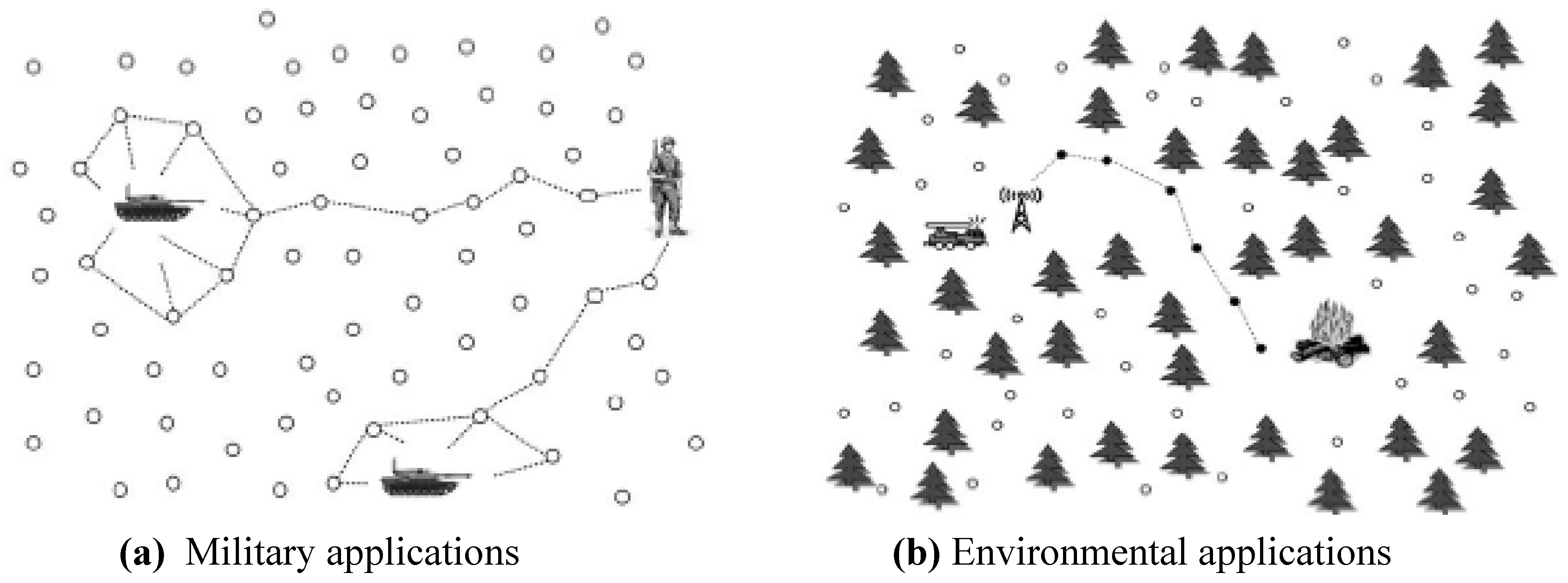
:1. Introduction

2. Related works
2.1 Locating sensors
2.2 Coverage and Connectivity
3. Routing algorithms based on sensor position
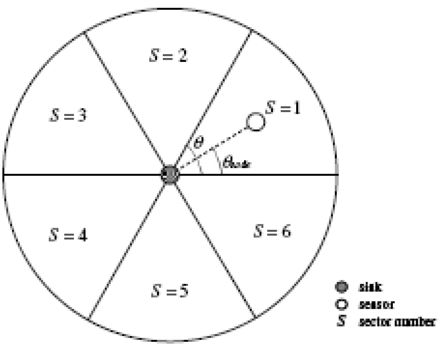
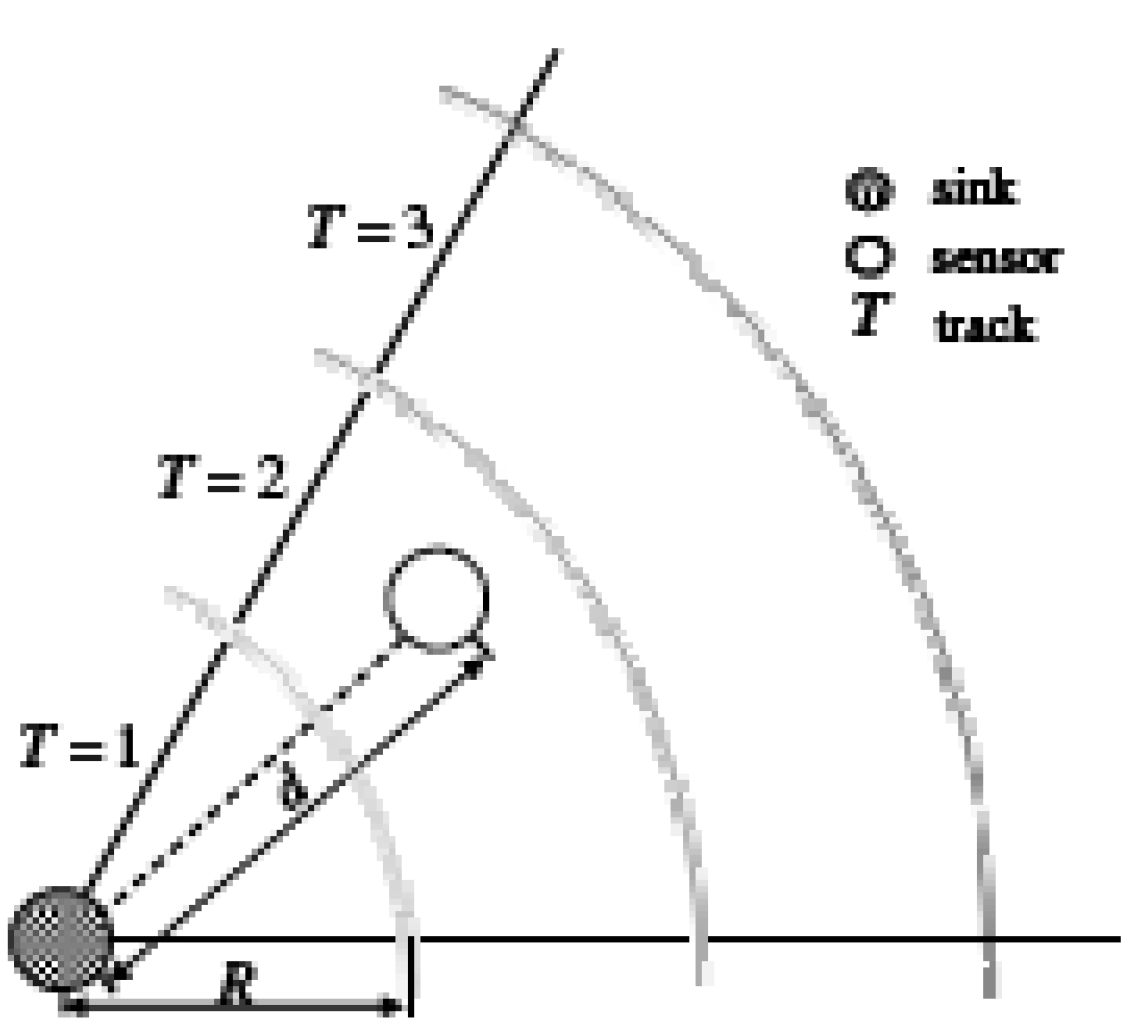
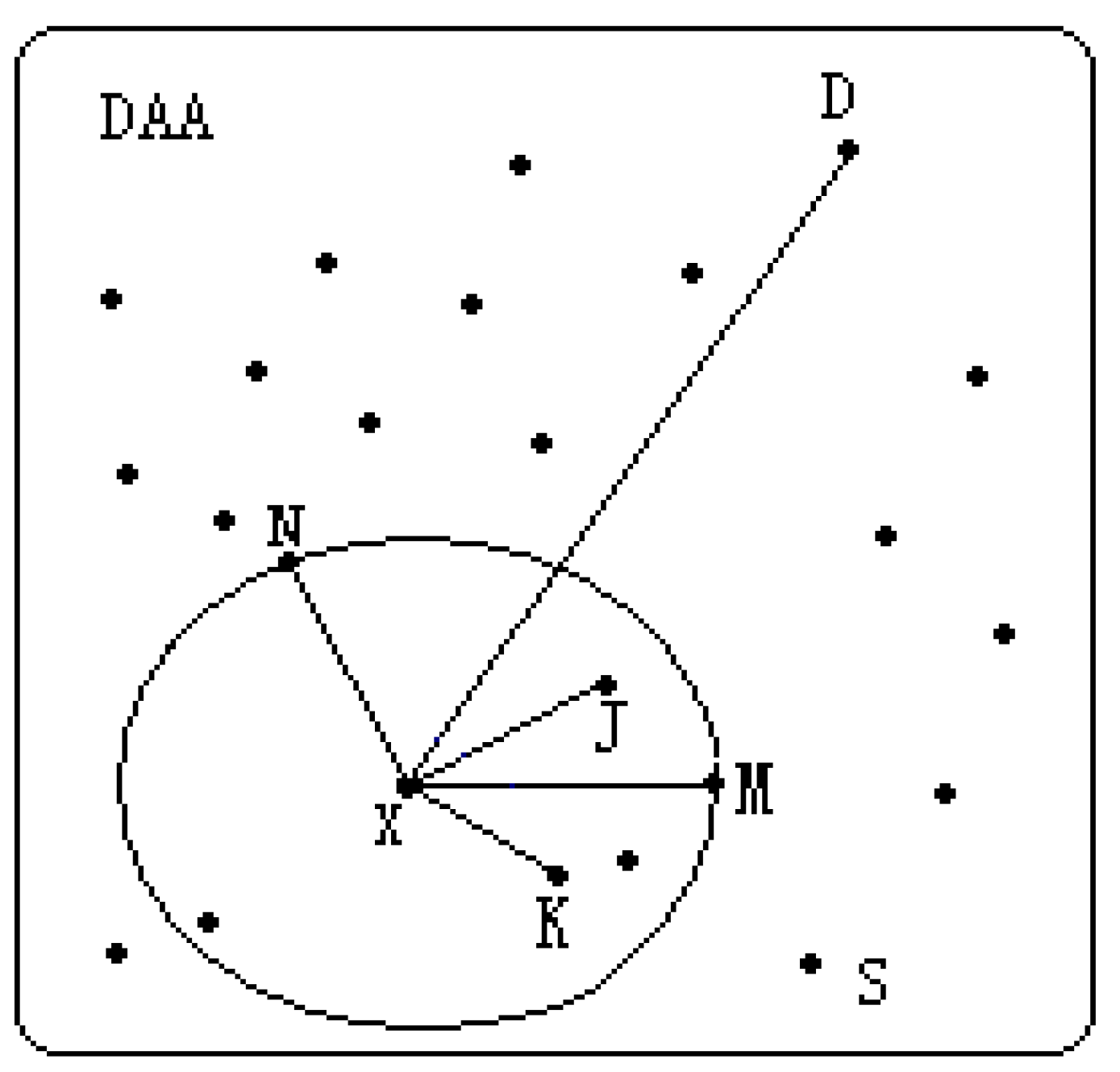
3.1 Flooding-based routing


| Random flooding | Rumor Routing | Limited flooding | |
| Energy consumption | Low | Middle | High |
| Negotiation-based | No | Yes | No |
| Complexity | Low | Low | Low |
| Reliability | No | Yes | Yes |
| Scalability | Middle | Good | Low |
| Multipath | No | Yes | Yes |
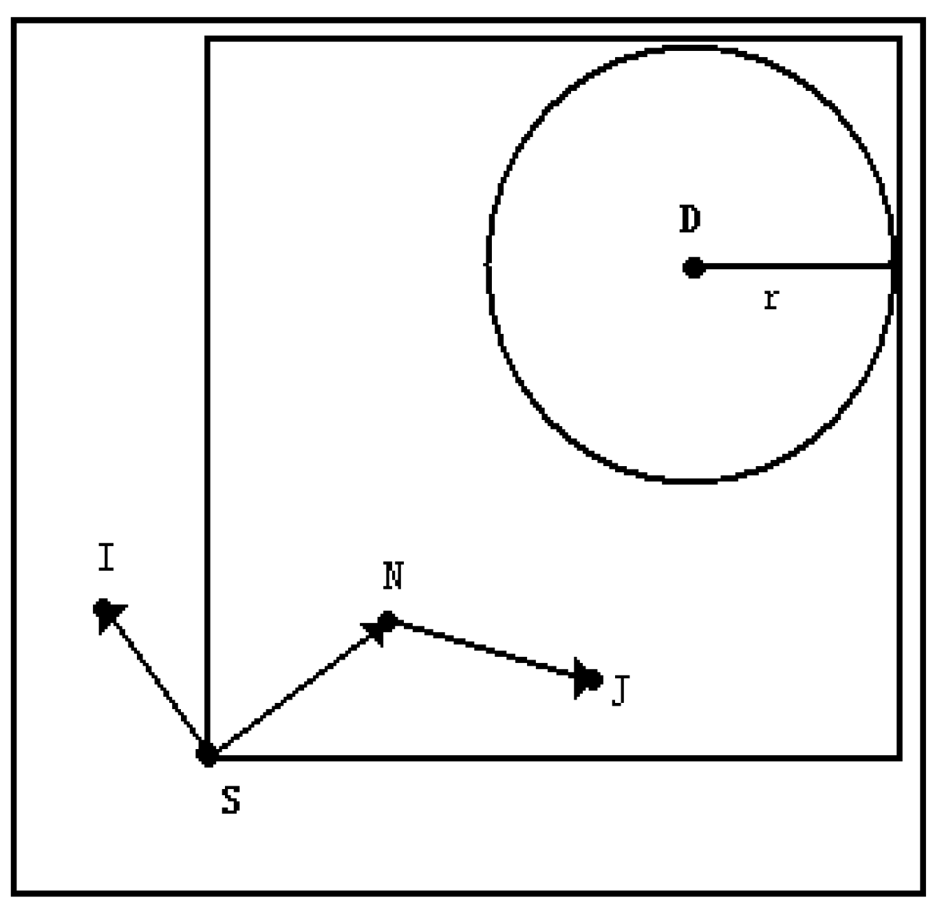
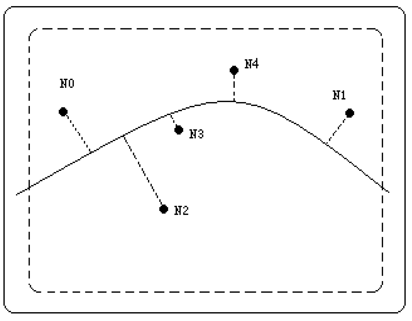
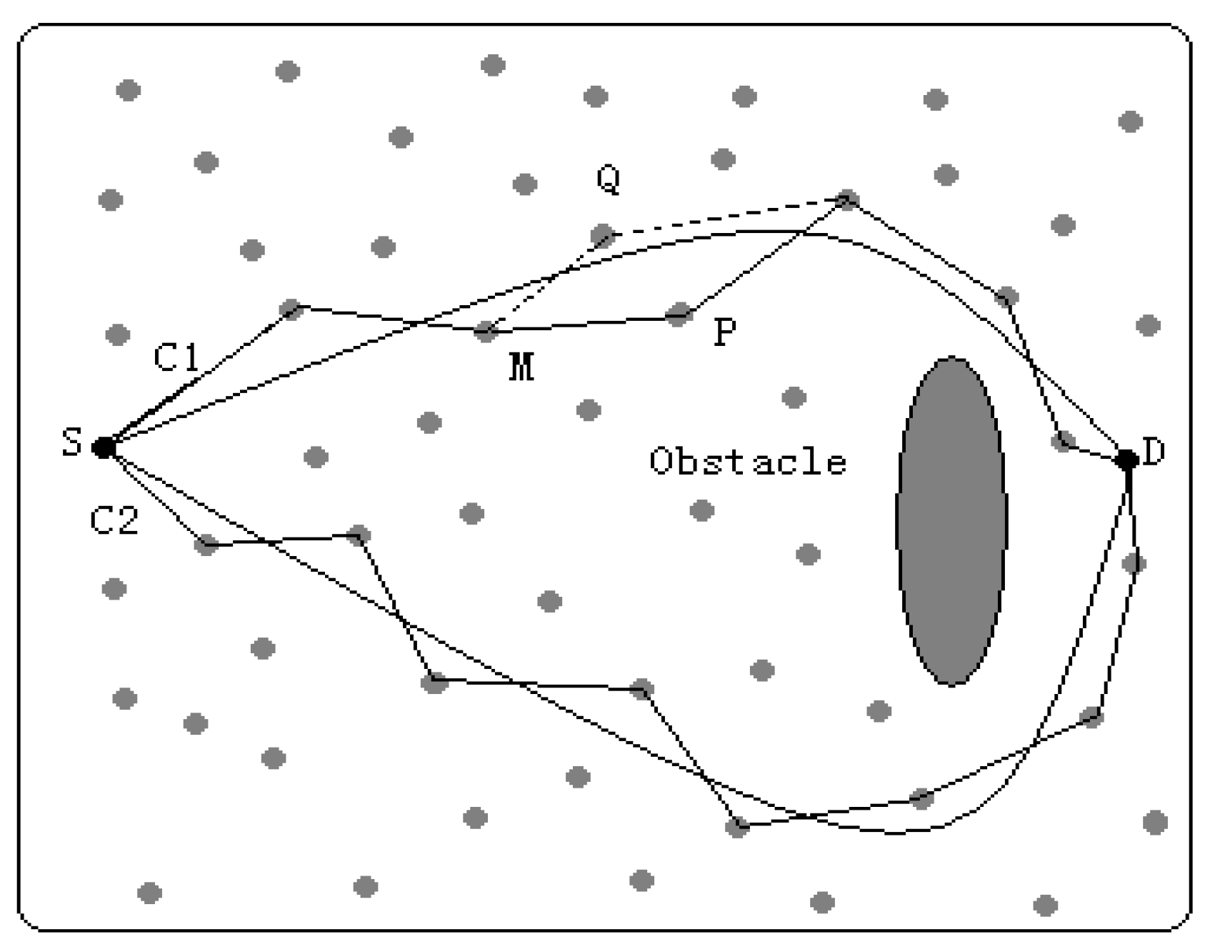
3.2 Curve-based routing


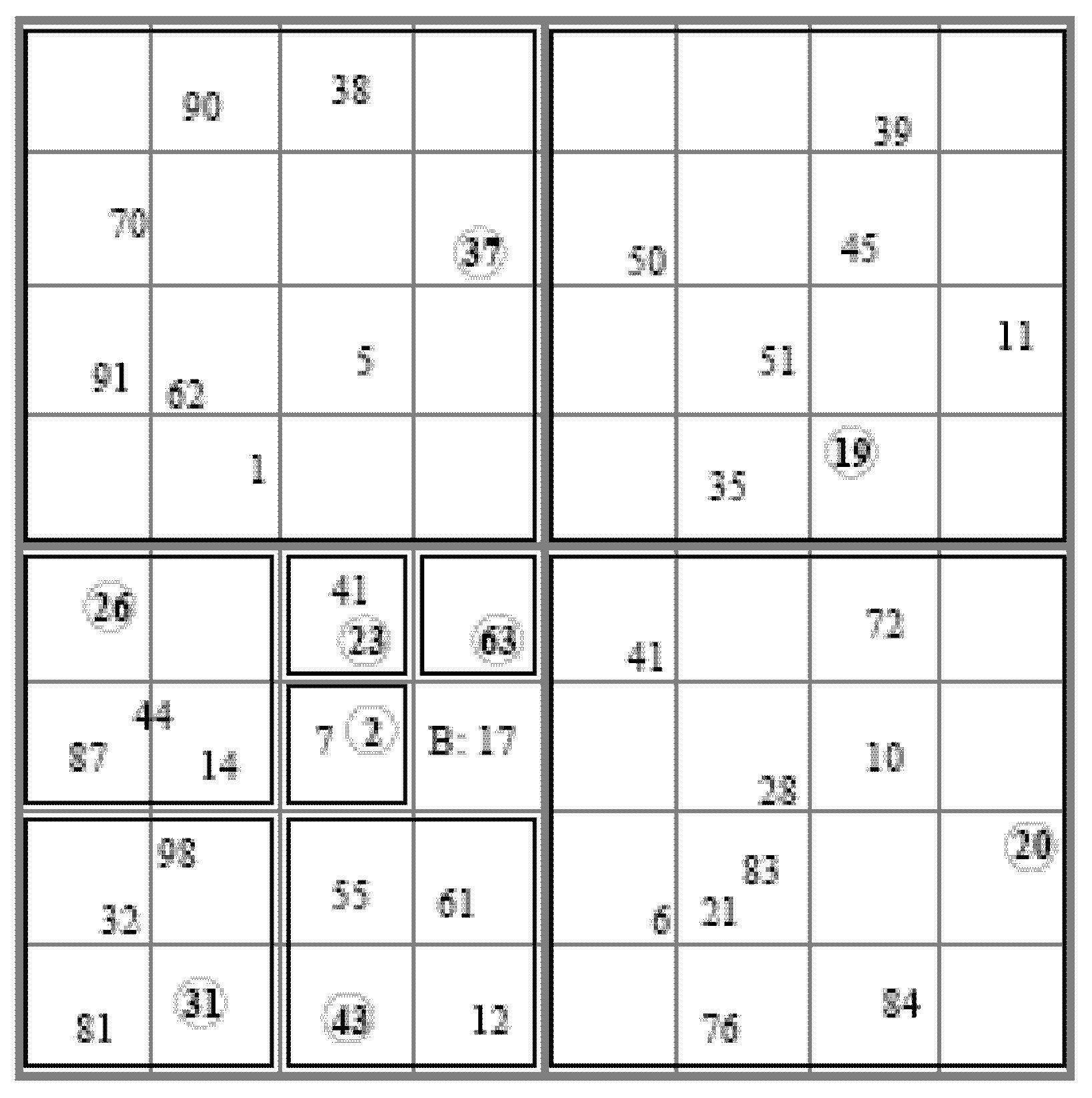
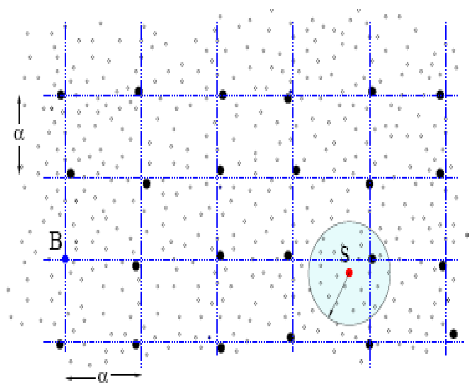
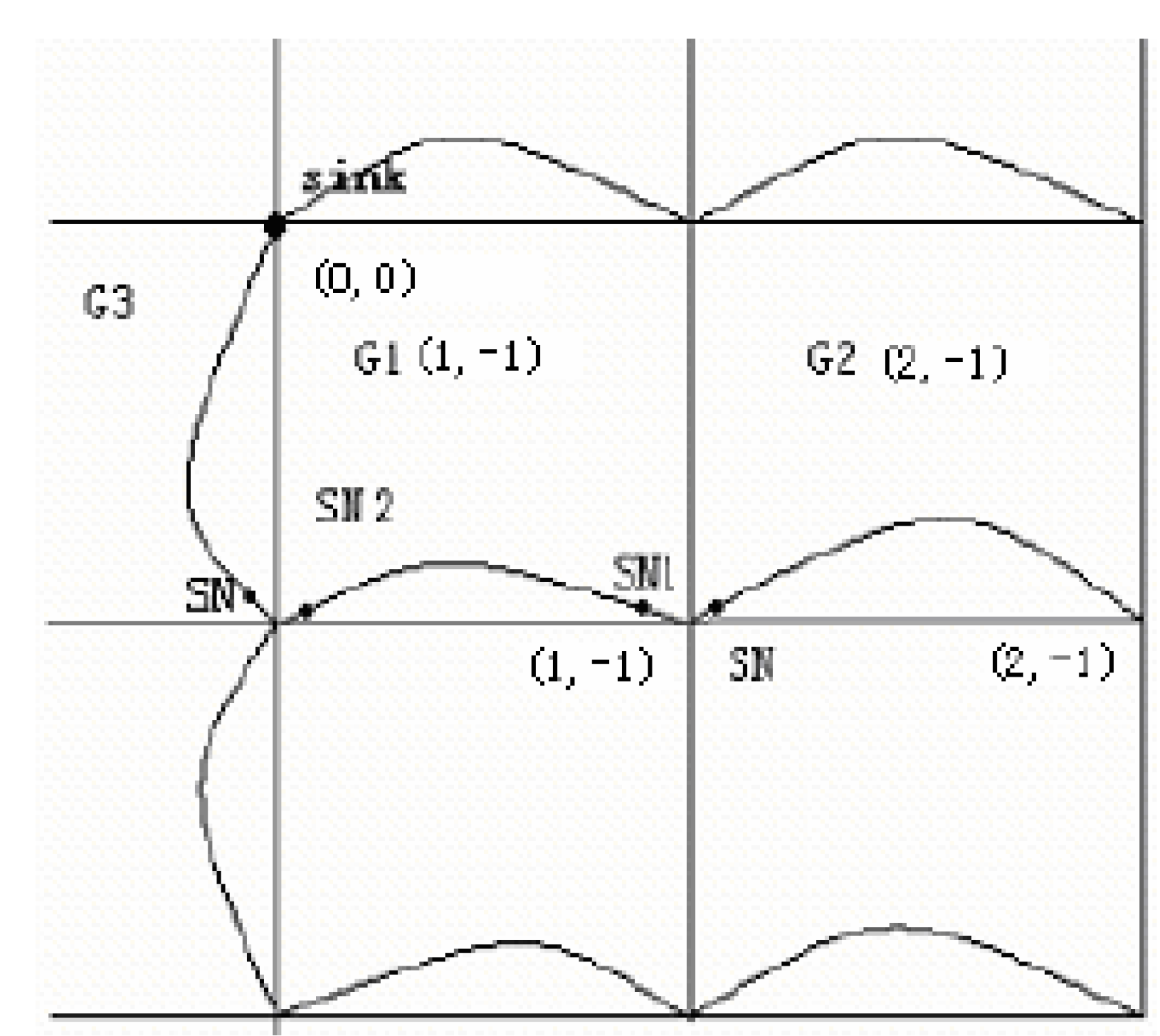
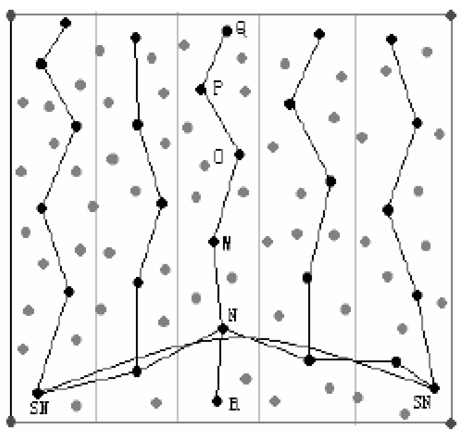
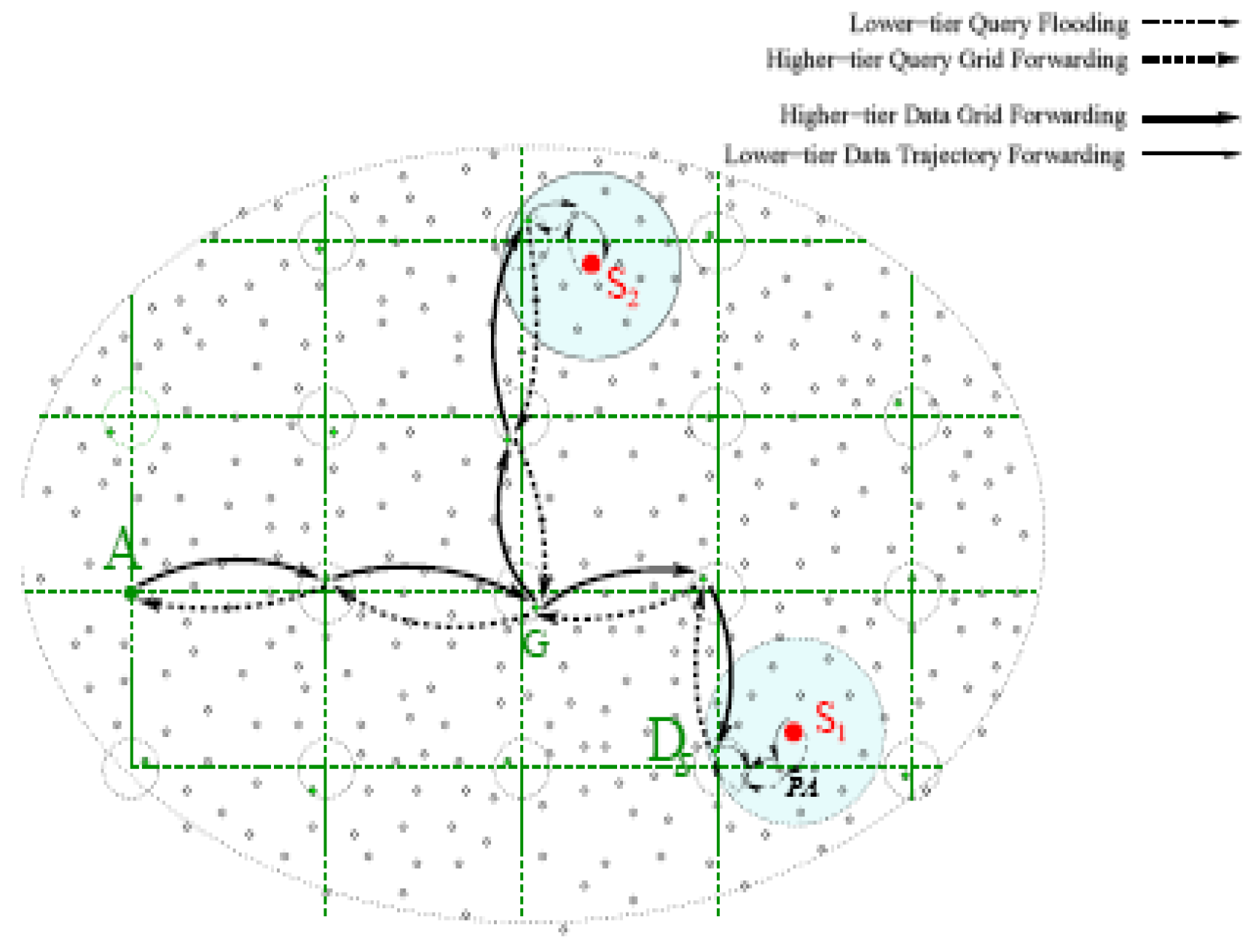
3.3 Grid-based routing


| GLS | TTDD | GBRA | |
| Energy consumption | High | Middle | Low |
| Negotiation-based | No | Yes | Yes |
| Complexity | High | Middle | Low |
| Reliability | High | Middle | Middle |
| Scalability | Low | Good | Middle |
| Mobility | All moving | Sink moving | No |
3.4 Ant algorithm-based intelligent routing
- ♦
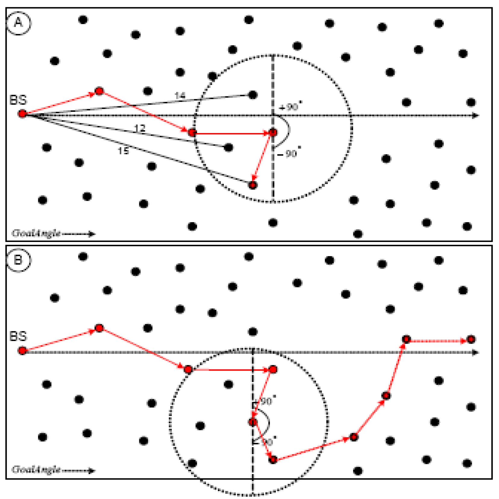
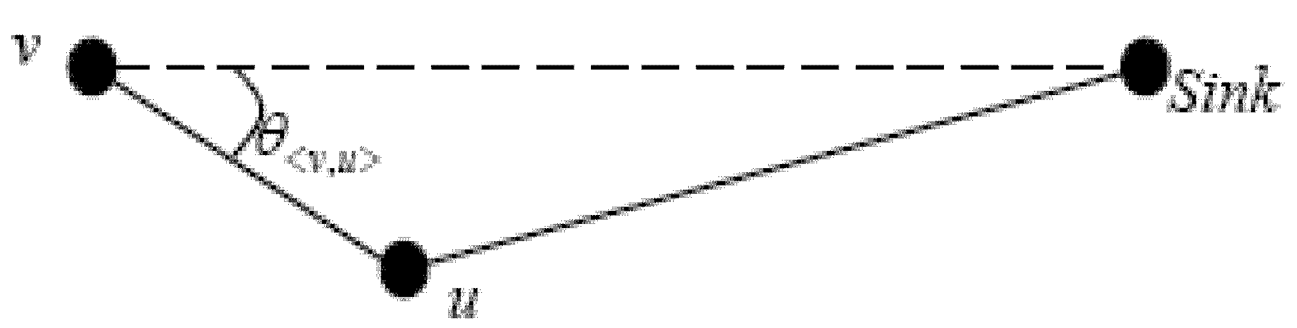
- Based on the coordinates of node v, node and the sink node, calculate the cosine value of angle by the formula of cosines. Then calculate the diverted weight of the node :, where the is the pheromone value of the edge ;
- ♦
- Select the neighbor node which holds the largest diverted value as the next hop node. If there are several nodes satisfied the condition , choose the node which owned the longest edge () as the next hop node.
3.5 Performance comparison
| Flood-based | Curve-based | Grid-based | Ant algorithm-based | |
| Energy consumption | High | Low | Low | Middle |
| Negotiation-based | No | No | Yes | Yes |
| Complexity | Low | Low | Middle | High |
| Reliability | High | Middle | Middle | Middle |
| Scalability | Low | Good | Good | Middle |
| Multipath | Yes | Yes | No | Possible |
| Data aggregation | No | No | Possible | No |
| Query-based | No | No | No | Yes |
4. Conclusion and Open Issues
- (1)
- The redundancy detection mechanism. In WSN, node is typically dense deployment. It is unnecessary that all these sensors simultaneously work. How to control the number of working sensors is valuable. Especially, the strategy combining the coverage algorithms with routing technology is hopeful. Another interesting idea is exploiting effective sensor-density control algorithms.
- (2)
- The secure routing problem. Security is very difficult to assure because the unsymmetrical encryption strategy is unsuitable for the energy requirement. Only the symmetrical encryption strategy can be used, which also make key assignment and time synchronization difficult. Most of current routing algorithms aim to optimize the energy consumption. Though there are some security strategies for routing, more attention still needs to be paid to satisfy the application requirement, such as battlefield environment.
- (3)
- QoS routing problem. To the video and imaging sensors and real-time applications, QoS routing in WSN should ensure suitable bandwidth (or delay) through the duration of connection as well as providing the use of most energy efficient path. Currently, there is very little research on routing strategy with QoS requirements in resource constrained environment, which is also a challenge task.
- (4)
- Intelligent routing mechanism. In WSN, most effort aims to design simple routing strategy, which is easy to realize and energy-aware. Considering those complicated application requirements, the intelligent routing technology is suitable when the sensors have more usable resources. Combining with position information, it’s hopeful to design the energy-aware intelligent routing.
- (5)
- Node mobility problem. Most of the current protocols assume that the sensor nodes are stationary. However, the moving sink or sensors can not be avoided in some special applications, which make nodes’ position change frequently. If the node position is updated frequently or not is a problem. New position-based routing ideas are needed in order to balance the topology update and the energy consumption.
- (6)
- Data fusion strategy. As an energy-aware operation, data fusion or aggregation is important and popular in hierarchical routing. Though most position-based routing algorithms are flat routing, it seems that data fusion is hard to use. Considering the grid-based routing algorithms, there are natural clusters making data fusion. How to realize data fusion in one grid is also an interesting problem to explore.
Acknowledgements
References
- Akyildiz, I.F.; Su, W.; Sankarasubramaniam, Y.; Cayirci, E. Wireless sensor networks: a survey. Computer Networks 2002, 38(4), 393–422. [Google Scholar] [CrossRef]
- Kahn, J. M.; Katz, R.H.; Pister, K.S.J. Next century challenges: mobile networking for smart dust. In Proceedings of ACM MobiCom, Seattle; 1999; pp. 271–278. [Google Scholar]
- Xiao, Renyi; Wu, Guozheng. A survey on routing in wireless sensor networks. Progress in natural science 2007, 17(3), 261–269. [Google Scholar]
- Jamal, N. Al-Laraki; Ahmed, E. Kamal. Routing techniques in wireless sensor networks: a survey. IEEE wireless communication 2004, 11(6), 6–28. [Google Scholar]
- Stojmenovic, I. Handbook of sensor networks: algorithms and architectures; John Wiley & Sons: New York, NY, USA, 2005. [Google Scholar]
- Delin, L.A.; Jackson, S.P.; Johnson, D.W.; Burleigh, S.C.; Woodrow, R.R.; McAuley, M.; Britton, J.T.; Dohm, J.M.; Ferré, T.P.A.; Felipe, I.; Rucker, D.F.; Baker, V.R. Sensor web for spatio-temporal monitoring of a hydrological environment. In Proceedings of Lunar and Planetary Science Conference, League City; 2004; pp. 1430–1438. [Google Scholar]
- Hill, J.; Szewczyk, R.; Woo, A. System architecture directions for networked sensors. In Proceedings of ASPLOS-IX, Cambridge; 2000; pp. 1–18. [Google Scholar]
- Perrig, A.; Szewczyk, R.; Tygar, J.D. SPINS: Security Protocols for Sensor Networks. Wireless Networks 2002, 8, 521–534. [Google Scholar] [CrossRef]
- Corke, P.; Hrabar, S.; Peterson, R.; Rus, D.; Saripalli, S.; Sukhatme, G. Autonomous deployment and repair of a sensor network using an unmanned aerial vehicle. In Proceedings of IEEE International Conference on Robotics and Automation, Kenmore; 2004; pp. 3602–3608. [Google Scholar]
- Callaway, E.H. Wireless Sensor Networks: Architectures and Protocols; CRC Press: Boca Raton, FL, USA, 2004. [Google Scholar]
- Akkaya, K.; Younis, M. A survey on routing protocols for wireless sensor networks. Ad Hoc Networks 2005, 3, 325–349. [Google Scholar] [CrossRef]
- Langendoen, K.; Reijers, N. Distributed localization in wireless sensor networks: a quantitative comparison. Computer Networks 2003, 43(4), 499–518. [Google Scholar] [CrossRef]
- Mao, G.; Barıs¸, F.; Anderson, B.D.O. Wireless sensor network localization techniques. Computer Networks 2007, 51(10), 2529–2553. [Google Scholar] [CrossRef]
- Koks, D. Numerical calculations for passive geolocation scenarios. Tech. Rep. DSTO-RR-0000, 2005. [Google Scholar]
- Rappaport, T.; Reed, J.; Woerner, B. Position location using wireless communications on highways of the future. IEEE Communications Magazine 1996, 34(10), 33–41. [Google Scholar] [CrossRef]
- Niculescu, D.; Nath, B. Ad hoc positioning system (APS) using AoA. In Proceedings of INFOCOM, San Francisco; 2003; pp. 1734–1743. [Google Scholar]
- Schmidt, R. Multiple emitter location and signal parameter estimation. IEEE Transactions on Antennas and Propagation 1986, 34(3), 276–280. [Google Scholar] [CrossRef]
- Roy, R.; Kailath, T. ESPRIT-estimation of signal parameters via rotational invariance techniques. IEEE Transactions on Acoustics, Speech, and Signal Processing 1989, 37(7), 984–995. [Google Scholar] [CrossRef]
- Priyantha, N.; Chakraborty, A.; Balakrishnan, H. The cricket location-support system. In Proceedings of the Sixth Annual ACM International Conference on Mobile Computing and Networking (MOBICOM), Boston; 2000; pp. 32–43. [Google Scholar]
- Savvides, A.; Han, C.-C.; Strivastava, M. B. Dynamic fine-grained localization in ad-hoc networks of sensors. In Proceedings of the 7th annual international conference on Mobile computing and networking (MobiCom), Rome; 2001; pp. 166–179. [Google Scholar]
- Prasithsangaree, P.; Krishnamurthy, P.; Chrysanthis, P. On indoor position location with wireless LANs. In Proceedings of 13th IEEE International Symposium on Personal, Indoor and Mobile Radio Communications, Lisbon; 2002; pp. 720–724. [Google Scholar]
- Bahl, P.; Padmanabhan, V. RADAR: an in-building RF-based user location and tracking system. In Proceedings of IEEE INFOCOM, Tel-Aviv; 2000; pp. 775–784. [Google Scholar]
- He, T.; Huang, C.; Blum, B. M.; Stankovic, J. A.; Abdelzaher, T. Range-free localization schemes for large scale sensor networks. In Proceedings of the 9th annual international conference on Mobile computing and networking (MobiCom), San Diego; 2003; pp. 81–95. [Google Scholar]
- Nagpal, R.; Shrobe, H.; Bachrach, J. Organizing a global coordinate system from local information on an ad hoc sensor network. In Proceedings of Second International Workshop on Information Processing in Sensor Networks (IPSN), Palo Alto; 2003; pp. 333–348. [Google Scholar]
- Niculescu, D.; Nath, B. Ad hoc positioning system (APS). In Proceedings of GLOBECOM, San Antonio; 2001; pp. 2926–293. [Google Scholar]
- Masoomeh, Rudafshani; Suprakash, Datta. Localization in wireless sensor networks. In Proceedings of the 6th International Conference on Information Processing in Sensor Networks, Cambridge,USA; 2007; pp. 51–60. [Google Scholar]
- Wu, J.; Li, H. A dominating-set-based routing scheme in ad hoc wireless networks. Telecommunication Systems Journal 2001, 18, 13–36. [Google Scholar] [CrossRef]
- Alzoubi, K. M.; Wan, P.-J.; Frieder, O. Message-optimal connected dominating sets in mobile ad hoc networks. In Proceedings of the International Symposium on Mobile Ad Hoc Networking and Computing (MobiHoc), Lausanne, Switzerland; 2002; pp. 157–164. [Google Scholar]
- Slijepcevic, S.; Potkonjak, M. Power efficient organization of wireless sensor networks. In Proceedings of the International Conference on Communications (ICC), Helsinki, Finland; 2001; pp. 472–476. [Google Scholar]
- Lin, F.Y.S.; Chiu., P. L. A near-optimal sensor placement algorithm to achieve complete coverage/discrimination in sensor networks. IEEE Communications Letters 2005, 9(1), 43–45. [Google Scholar]
- Tian, D; Georganas, N.D. A node scheduling scheme for energy conservation in large wireless sensor networks. Wireless Communications and Mobile Computing 2003, 3(2), 271–290. [Google Scholar] [CrossRef]
- Gupta, H; Das, S.R.; Gu, Q. Connected sensor cover: Self-Organization of sensor networks for efficient query execution. In Proceedings of the ACM International Symposium on Mobile Ad Hoc Networking and Computing(MobiHOC), Annapolis, USA; 2003; pp. 189–200. [Google Scholar]
- Heinzelman, W.; Kulik, J.; Balakrishnan, H. Adaptive protocols for information dissemination in wireless sensor networks. In Proceedings of the 5th Annual ACM/IEEE International Conference on Mobile Computing and Networking (MobiCom), Seattle, USA; 1999; pp. 174–185. [Google Scholar]
- Braginsky, D.; Estrin, D. Rumor routing algorithm for sensor networks. In Proceedings of the 1st ACM international workshop on wireless sensor networks and applications, Atlanta, USA; 2002; pp. 22–31. [Google Scholar]
- Banka, T.; Tandon, G.; Jayasumana, A.P. Zonal rumor routing for wireless sensor networks. In Proceedings of International Conference on Information Technology, Coding and Computing, Las Vegas, USA; 2005; pp. 562–567. [Google Scholar]
- Shokrzadeh, H.; Haghighat, A. T. Directed Rumor Routing in Wireless Sensor Networks. In Proceedings of ICEE, Iran; 2007. [Google Scholar]
- Shokrzadeh, H.; Haghighat, A. T.; Tashtarian, F.; Nayebi, A. Directional Rumor Routing in Wireless Sensor Networks. In Proceedings of 3rd IEEE/IFIP International Conference in Central Asia on Internet, Tashkent, Uzbekistan; 2007; pp. 1–5. [Google Scholar]
- Son, J.; Ha, N.; Kim, K.; Ryu, J.; Son, J.; Han, K. A Limited Flooding Scheme for Query Delivery in Wireless Sensor Networks. In Proceedings of International Workshop on Sensor Networks, volume 3842 of Lecture Notes in Computer Science, Harbin, China; 2006; pp. 276–280. [Google Scholar]
- Zhang, J. On Routing Algorithms Based on Position Information for Sensor Networks. Master dissertation, Hunan University, Changsha, 2004. [Google Scholar]
- Zhang, J.; Lin, Y. P. An Angle-Area-Based Flood Routing Algorithm for Sensor Networks. Computer Engineering & Science 2005, 27(9), 59–61. (In Chinese) [Google Scholar]
- Ko, Y. B.; Vaidya, N. H. Location-Aided Routing (LAR) in mobile ad hoc networks. Wireless Networks 2000, 6, 307–321. [Google Scholar] [CrossRef]
- Johnson, D. B.; Maltz, D. A. Dynamic source routing in ad hoc wireless networks. Mobile Computing 1996, 353, 153–181. [Google Scholar]
- Finn, G. Routing and addressing problems in large metropolitan-scale internetworks. Technical Report ISI Research Report ISI/RR-87-180, University of Southern California, March 1987. [Google Scholar]
- Niculescu, D.; Nath, B. Trajectory based forwarding and its applications. In Proceedings of 9th Annual International Conference on Mobile Computing and Networking, San Diego, USA; 2003; pp. 260–272. [Google Scholar]
- Zhang, J.; Lin, Y. P.; Lin, M.; Li, P.; Zhou, S. W. Curve-Based Greedy Routing Algorithm for Sensor Networks. In Proceedings of International Conference on Computer Network and Mobile Computing, Lecture Notes in Computer Science, Zhangjiajie, China; 2005; vol. 2619, pp. 1125–1133. [Google Scholar]
- Yuksel, M.; Pradhan, R.; Kalyanaraman, S. An Implementation Framework for Trajectory-Based Routing in Ad Hoc Networks. In Proceedings of IEEE International Conference on Communications’ 04, Paris, France; 2004; pp. 4062–4066. [Google Scholar]
- Cheng, F. H.; Zhang, J. A Reliable Routing Algorithm for Sensor Network Based on Multi-path. In Proceedings of 9th International Conference on Control, Automation, Robotics and Vision, Singapore; 2006; pp. 1–3. [Google Scholar]
- Li, J. Y.; Jannotti, J.; De, D. S. J.; David, C.; Karger, R.; Morris, R. A Scalable Location Service for Geographic Ad Hoc Routing. In Proceedings of the 6th ACM International Conference on Mobile computing and Networking (MobiCom'00), Boston, USA; 2000; pp. 120–130. [Google Scholar]
- Luo, H. Y.; Ye, F.; Cheng, J.; Lu, S. W.; Zhang, L. X. TTDD: Two-Tier Data Dissemination in Large-Scale Wireless Sensor Networks. Wireless Networks 2005, 11, 161–175. [Google Scholar] [CrossRef]
- Zhang, J.; Li, G. A Density-Based Energy-Effective Routing for Sensor Networks. In Proceedings of the 6th World Congress on Control and Automation, Chongqing, China; 2006; pp. 3801–3804. [Google Scholar]
- Peng, T. G.; Zhang, J. Grid-Based Routing Algorithm for Sensor Networks. In Proceedings of International Conference on Wireless Communications, Networking and Mobile Computing, Shanghai, China; 2007; pp. 2242–2245. [Google Scholar]
- Intanagonwiwat, C.; Govindan, R.; Estrin, D. Directed Diffusion: A Scalable and Robust Communication Paradigm for Sensor Networks. In Proceedings of ACM International Conference on Mobile Computing and Networking (MobiCom), Boston, USA; 2000; pp. 56–67. [Google Scholar]
- Ye, F.; Zhong, G.; Lu, S.; Zhang, L. GRAdient broadcast: a robust data delivery protocol for large scale sensor networks. Wireless Networks 2005, 11(3), 285–298. [Google Scholar] [CrossRef]
- Karp, B.; Kung, H. T. GPSR: Greedy perimeter stateless routing for wireless networks. In Proceedings of the Sixth Annual ACM/IEEE International Conference on Mobile Computing and Networking (MobiCom), Boston, USA; 2000; pp. 243–254. [Google Scholar]
- Dorigo, M.; Gambardella, L.M. Ant colonies for the traveling salesman problem. BioSystems 1997, 43(2), 73–81. [Google Scholar] [CrossRef]
- Yu, J.P.; Lin, Y.P.; Lin, M.; Yi, Y.Q. Multi-constrained anycast routing based on ant algorithm. Chinese Journal of Electronics (CJE) 2006, 15(1), 133–137. [Google Scholar]
- Yu, J.P.; Lin., Y.P.; Zheng, J.H. Ant-based query processing for replicated events in wireless sensor networks. In Proc of the 2008 IEEE World Congress on Computational Intelligence (IEEE WCCI 2008), Hongkong, China; 2008; pp. 138–145. [Google Scholar]
- Dorigo, M.; Birattari, M.; Stützle, T. Ant colony optimization-Artificial ants as a computational intelligence technique. IEEE Computational Intelligence Magazine 2006, 1(4), 28–39. [Google Scholar] [CrossRef]
- Li, W.; Lin, Y.P.; Tong, T.S.; Chen, Y.; Yu, J.P. A distributed data-centric routing algorithm based on ant algorithm for sensor networks. Mini-Micro Systems 2005, 26(5), 788–792. (In Chinese) [Google Scholar]
- Li, S.; Yang, C.; Kang, J. An ant algorithm for data broadcasting and gathering in the sensor network. Jounal of Wuhan University (Natural Science Edition) 2006, 52(1), 100–104. (In Chinese) [Google Scholar]
- Liao, W. H.; Kao, Y. C.; Fan, C. M. Data aggregation in wireless sensor networks using ant colony algorithm. Journal of Network and Computer Applications 2008, 31(4), 387–401. [Google Scholar] [CrossRef]
© 2009 by the authors; licensee Molecular Diversity Preservation International, Basel, Switzerland. This article is an open-access article distributed under the terms and conditions of the Creative Commons Attribution license (http://creativecommons.org/licenses/by/3.0/).
Share and Cite
Jin, Z.; Jian-Ping, Y.; Si-Wang, Z.; Ya-Ping, L.; Guang, L. A Survey on Position-Based Routing Algorithms in Wireless Sensor Networks. Algorithms 2009, 2, 158-182. https://doi.org/10.3390/a2010158
Jin Z, Jian-Ping Y, Si-Wang Z, Ya-Ping L, Guang L. A Survey on Position-Based Routing Algorithms in Wireless Sensor Networks. Algorithms. 2009; 2(1):158-182. https://doi.org/10.3390/a2010158
Chicago/Turabian StyleJin, Zhang, Yu Jian-Ping, Zhou Si-Wang, Lin Ya-Ping, and Li Guang. 2009. "A Survey on Position-Based Routing Algorithms in Wireless Sensor Networks" Algorithms 2, no. 1: 158-182. https://doi.org/10.3390/a2010158