High Frequency Waves Propagating in Octagonal Bars: a Low Cost Computation Algorithm

Abstract

In this paper a hybrid semi-analytical Finite Element formulation is proposed to efficiently calculate the time dependent response due to stress waves propagating in a slender solid with uniform cross-section when excited by impulsive forces. The formulation takes advantage of the direct and inverse Fourier transform to formulate and solve the governing wave equation. The framework is applied to an octagonal viscoelastic isotropic steel bar.

1. Introduction

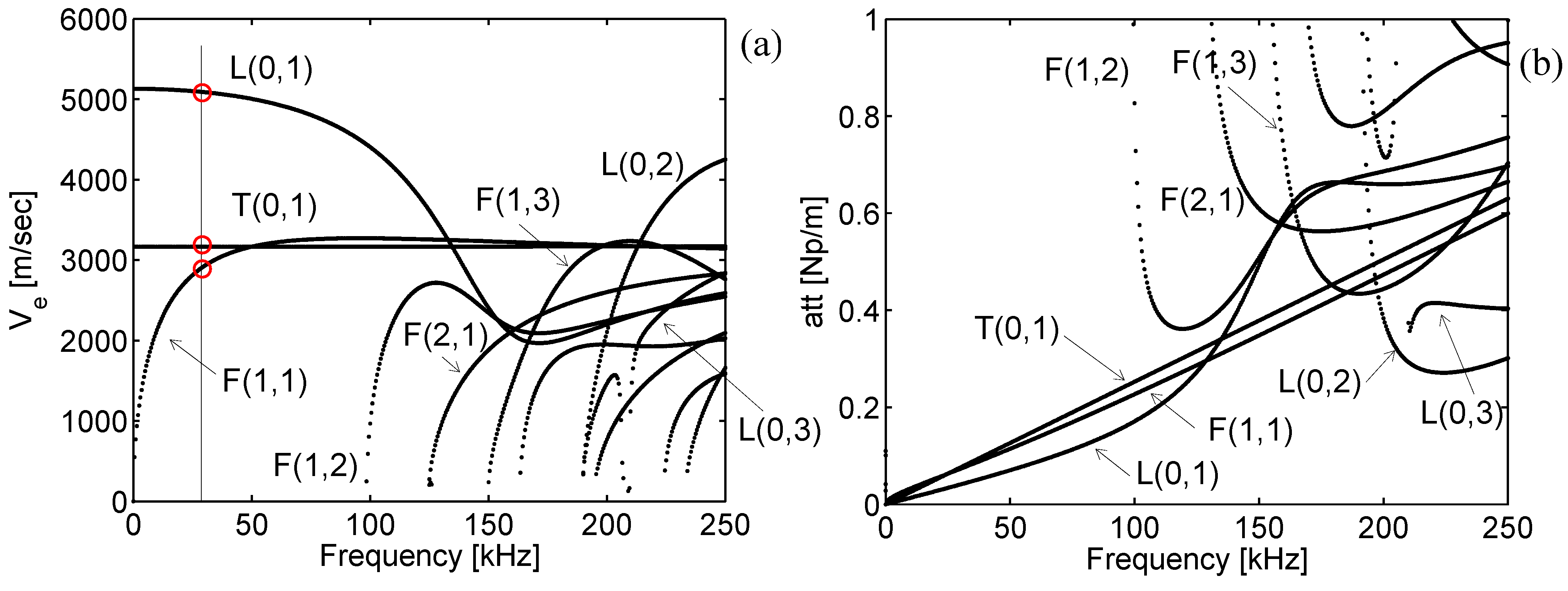
A force with a high frequency content acting at a point on a slender solid with uniform cross section (waveguide) generates mechanical waves. These waves, generally termed as Guided Waves (GWs) due to the fact that the solid serves as a waveguide, propagate with defined wavelength, phase velocity, energy velocity, attenuation and wavestructure (wave shape over the waveguide cross-section). Due to the interaction between the wave’s wavelength and the waveguide cross-section geometry, some or all of these wave features change when varying the frequency of propagation (dispersive behavior). Today, GWs are employed in several industrial applications for material characterization, impact and shock-induced wave propagation, acoustic focusing and advanced material design. Modeling these propagating waves in complex waveguides is not an easy task, especially at high frequency, where the wavelengths are small and the wavestructures have a complex shape.

Among others, Spectral Finite Element (SFE) formulations are well established algorithms to simulate guided waves propagating in waveguides. The key point of SFE formulations consists in the hybrid displacement field adopted to describe the motion of a propagative guided wave. A transient wave is described, in fact, coupling a bi-dimensional finite element mesh over the waveguide cross-section and harmonic functions along the wave propagation direction. Next, a displacement-based variational scheme and the application of Fourier transform contractions leads to the governing wave equation in the frequency-wavenumber domain as a system of algebraic equations. Non trivial solutions of the homogenous part of the wave equation, easily calculated by using standard routines for eigenvalue problems, allow tracing the dispersive spectrum of the waveguide. Compared to other methods the main advantages in this calculation are: no missing roots; capability to handle waveguides of arbitrary cross-section; possibility to model high degree anisotropic waveguides with no extra effort; fast and reliable high frequency computation. A literature review on SFE formulations, acknowledged also as semi-analytical finite element (SAFE) formulations or waveguide finite element (WFE) methods, can be found in the book by Liu and Xi [1].

The SFE calculated waveguide spectrum, can also be exploited for the construction of the time-transient response due to the waves excited by a time-varying load. Time-transient response is essential to actuators design, quantitative non-destructive evaluation of cracks size and location as well as for structural health monitoring purposes. In brief, the time-transient response at a point can be obtained by means of the inverse Fourier transform, which turns into the time domain the waveguide frequency response calculated as a summation of the modal data contribution at that point weighted with the spectrum of the applied load. Applications of this procedure to calculate the time-transient response in undamped waveguides, such as plates [2] and pipes [3], have been proposed in the past.

Lately, some work has been devoted to extend SFE procedures to damped waveguides. In particular Bartoli et al., [4] generalized the SFE formulation to compute the modal spectrum in lossy waveguides by accounting for material damping, at the finite element level, by introducing complex constitutive viscoelastic relations.

The scheme proposed in [4] has been next used to extract the damped dispersion curves in pipes [5] and helical waveguides [6], and subsequently exploited to extend SFE formulations to the calculation of the time-transient response in damped pipes [7] and rails [8].

In particular, in [7] where the scheme proposed in [4] was fully used, the SFE formulation is based on the analytical derivation of the complex stiffness matrices from the material acoustic properties. This also allows handling of frequency dependent linear viscoelastic rehological models, once the bulk properties are known. However, since the formulation in [7] was purposely developed for damped axially symmetric waveguides it is limited to them.

The formulation proposed in [8], can also deal with waveguides with generic cross section. However, the damping is simply introduced by adding an imaginary “stiffness” proportional to real “stiffness”, simulating thus a sort of hysteretic material for the waveguide.

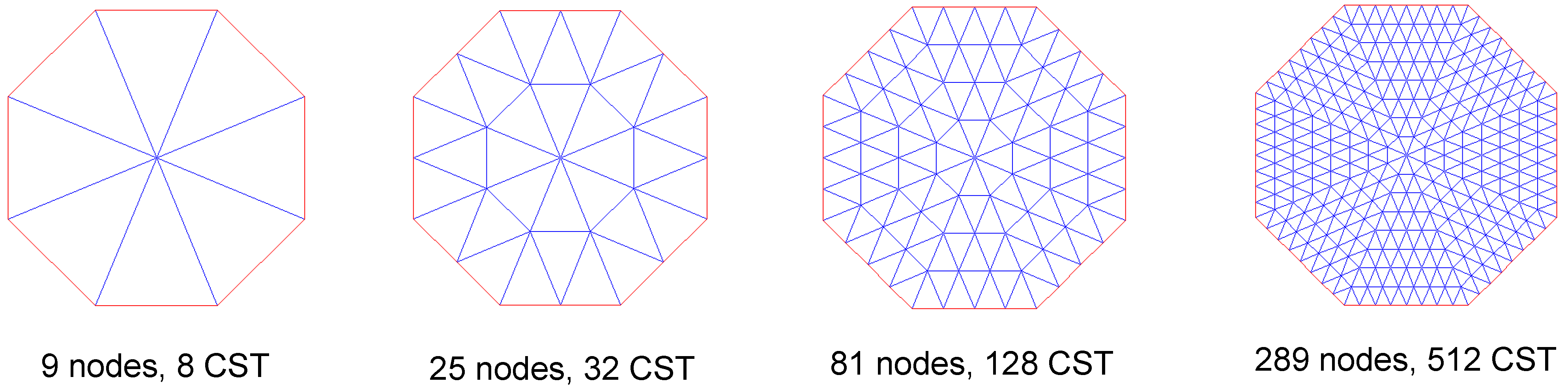
Herein, a damped spectrally formulated plane triangular finite element with constant strain description (CST) is proposed to extend the formulation in [7] to waveguides of arbitrary cross-section. Damping is accounted analytically starting from the damped bulk properties of the material.

The proposed algorithm can thus provide the dispersion curves as well as calculate the time transient response in waveguides of arbitrary cross-section accounting for any linear viscoelastic constitutive model that can be formulated in the frequency domain.

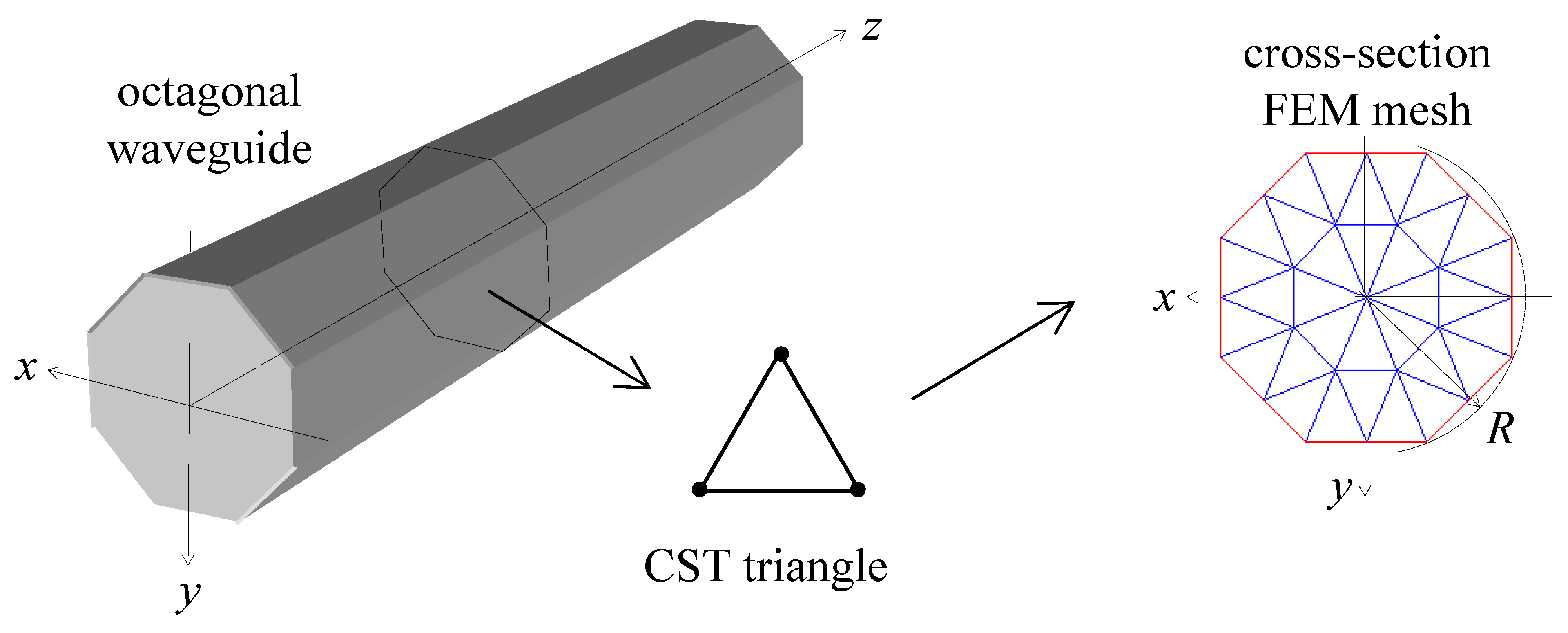
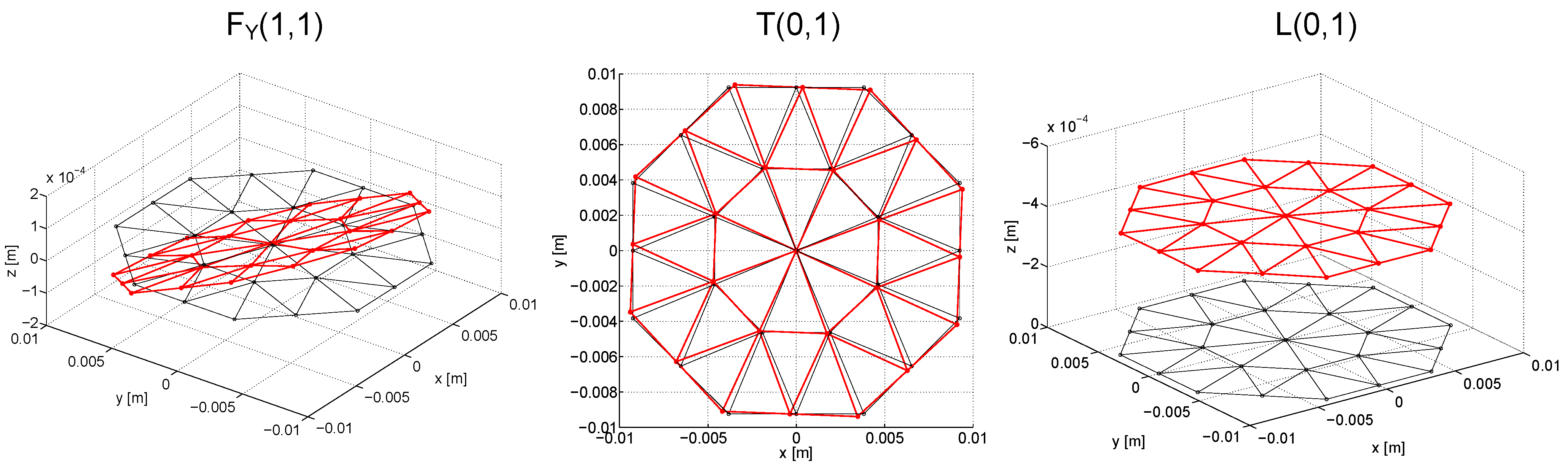
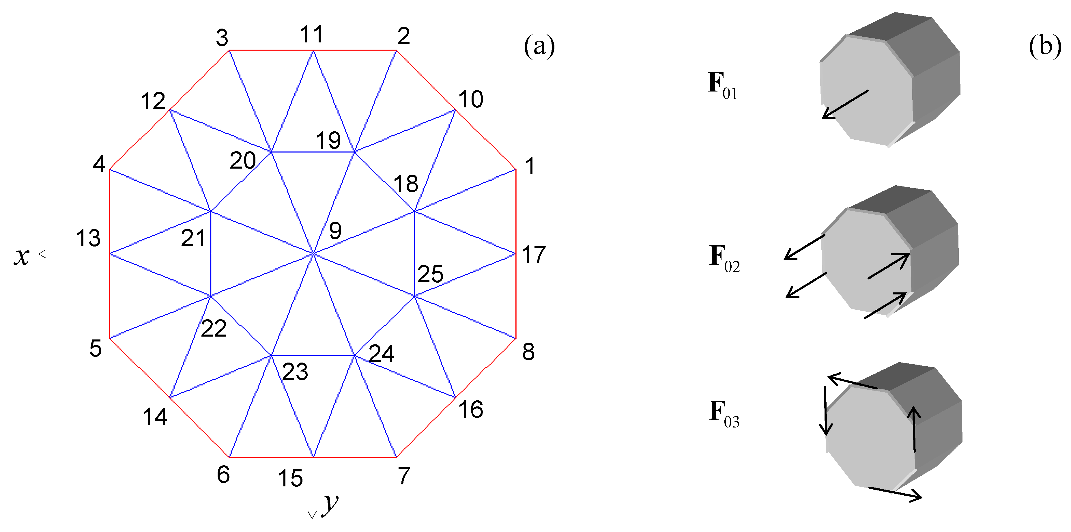
The formulation is next adopted to analyze the problem of guided waves propagating in octagonal damped bars that to the authors’ best knowledge has never been addressed. Octagonal bars, having a generic cross section, are representative of any arbitrary cross section waveguide and therefore useful to prove the reliability of the formulation. In addition since an octagonal bar has a behavior somehow similar to the one well-known of an equivalent rod with circular cross-section, the formulation and its results were controlled by means of the algorithm developed in [5] for axially symmetric waveguides.

Finally, stress waves in octagonal bars are of interest since they can reveal some useful information on the behaviour of guided waves propagating in octagonal tubes, largely used for highway signal marks and lighting poles. These structures present two critical regions that are susceptible of corrosion because of the deposit of water: the base of the pole at the street level and the underground zone where the pole joins the concrete foundation. While the base of the pole can be rapidly inspected in several ways, the screening of the underground zone presents more difficulties.

Therefore, a guided waves based non-destructive technique that operating from the outside near surface is capable to reveal the state of corrosion in the underground zone could be really appealing. Here, the basis for the numerical simulation are set. In this study several cases have been investigated to show the performance of the proposed procedure by considering different source-receiver distances and different excitations.

1.1. Matlab Overall Strategy

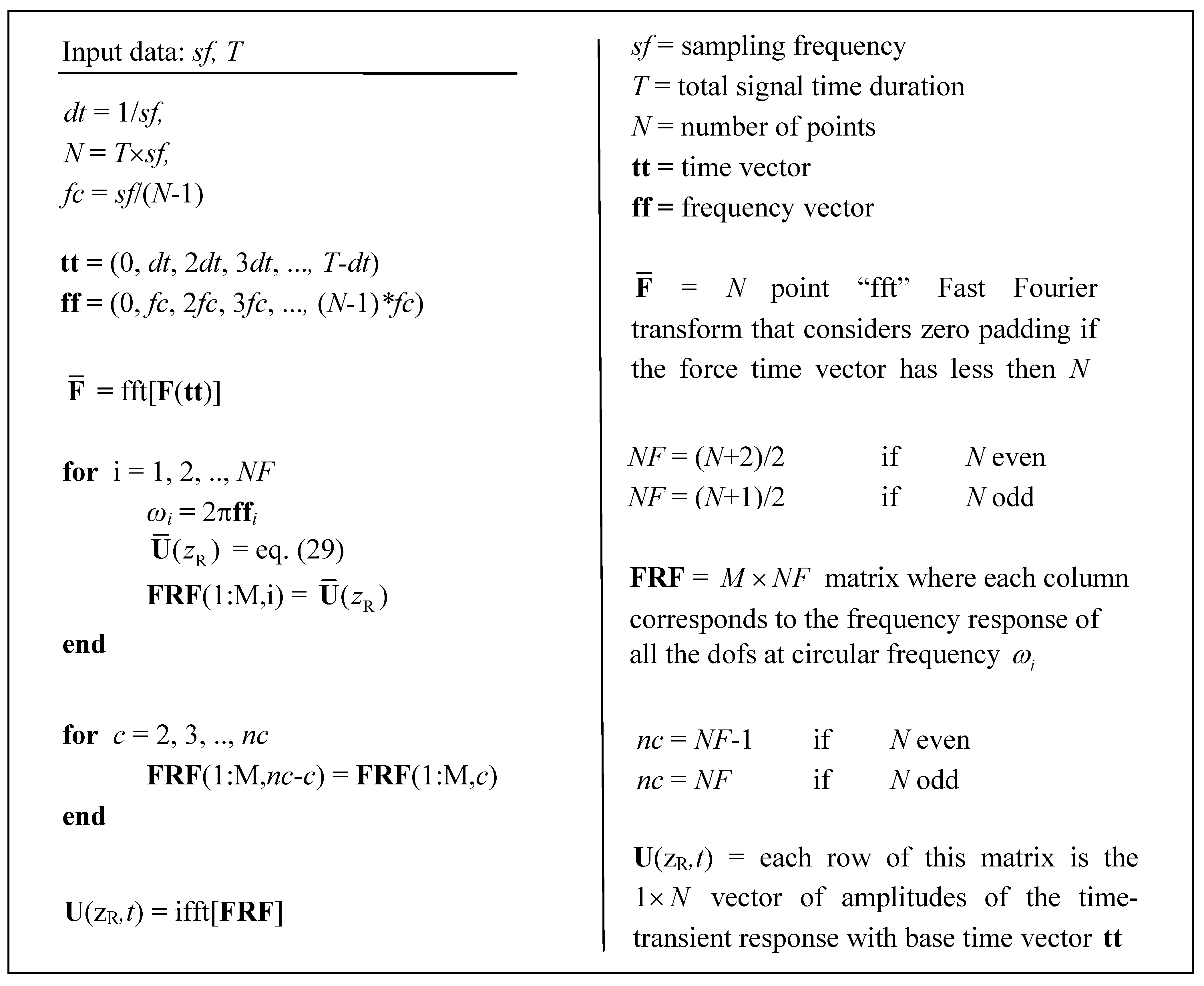
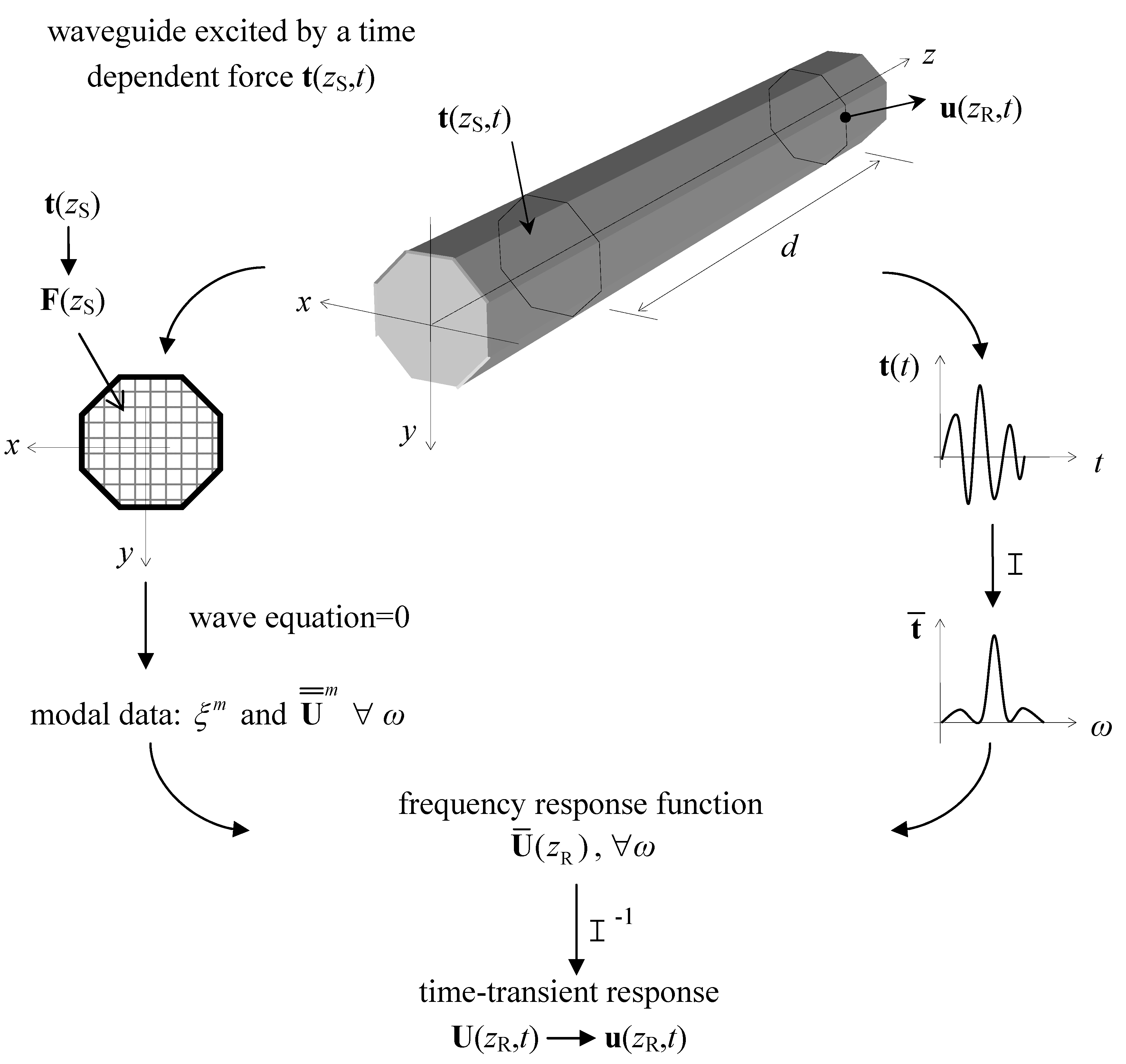
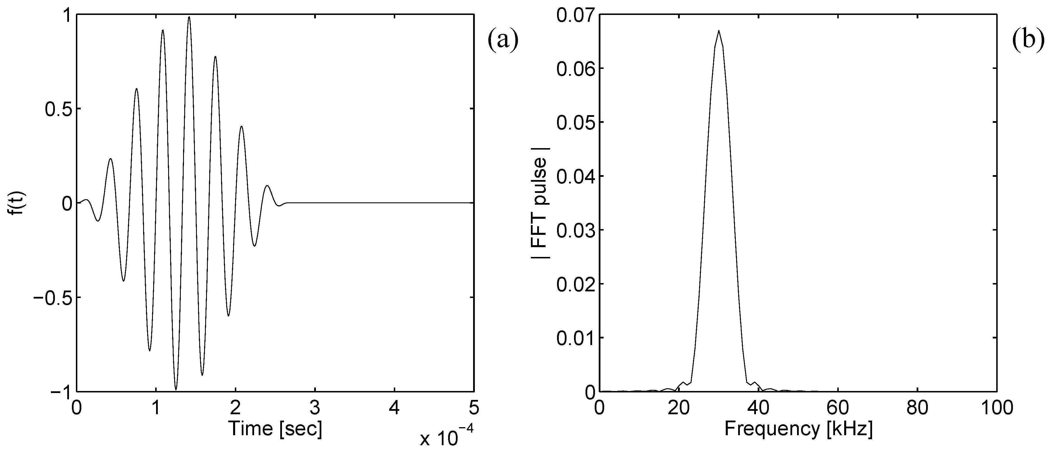
The procedure for the construction of the damped time-transient response is described in the following. First, home made routines are developed to set the spectral damped CST finite element. The “pdetool” of Matlab is next used to draw the cross-section of the waveguide and to create the plane finite element mesh data. Then, a standard finite element assembly procedure generates the frequency-wavenumber dependent homogeneous governing wave equation. In parallel, the applied forcing function at a certain z-coordinate $t(z_{\text{S}},t)$ (where the subscript S stands for source location) is discretized over the finite element mesh $F(z_{\text{S}})$ and its frequency spectrum $\overline{t}=t(\omega )$ is calculated by means of the “fft” function of Matlab.

For a given frequency in input ($\omega =2\pi f$), the solution of the homogeneous form of the wave equation using the function “eig” leads to all the complex wavenumbers (${\xi }^m$) and wavestructures (${\overline{\overline{U}}}^m$) of the $m=1,2,3,\mathrm{...},2M$ existing waves at that frequency, where $M$ is the number of degrees of freedom (dofs) of the mesh. The waves phase/energy velocity and attenuation are calculated from these modal properties by means of simple formulae.

Figure 1. Schematic representation of the overall strategy.

Figure 1. Schematic representation of the overall strategy.

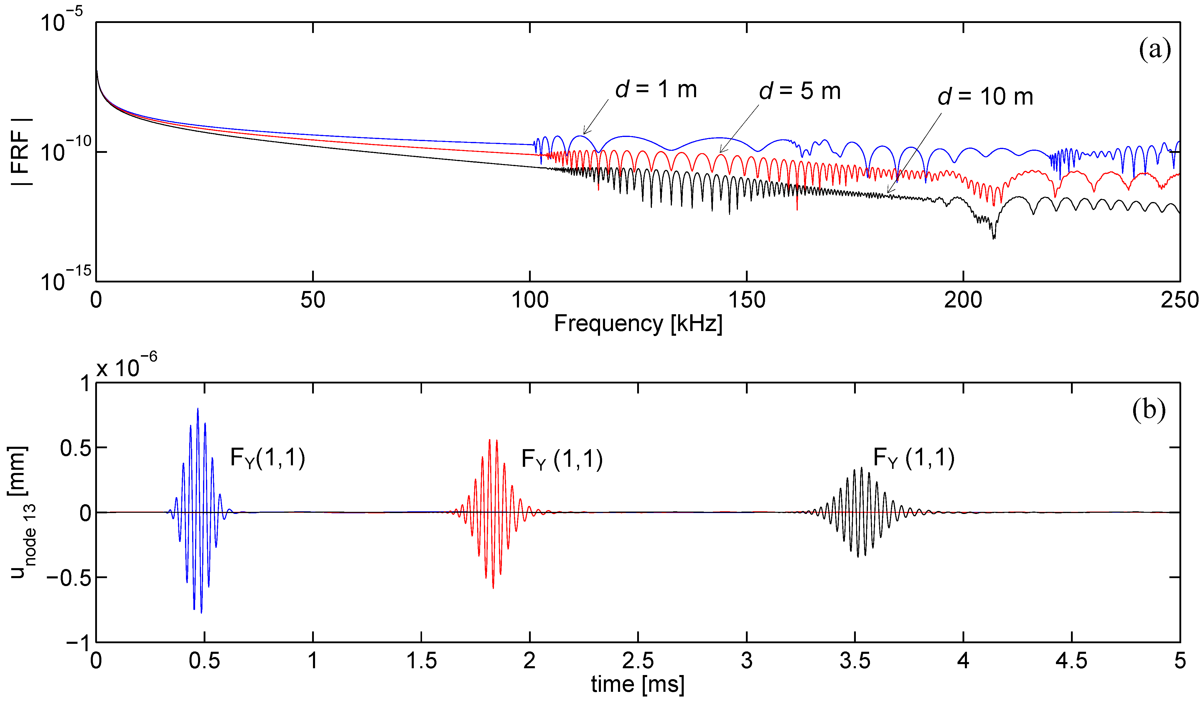
Also, the modal properties (ξ^m, ${\overline{\overline{U}}}^m$) weighted by the spectrum of the applied force at the given frequency $\overline{F}(z_S)=F(z_S)\overline{t}$ yield the waveguide frequency response $\overline{U}(z_{\text{R}})$ of all the mesh dofs at a distance $d=z_R-z_S$ away from the wave source (where the subscript R stands for receiver point). Repeating this procedure for all the frequencies of interest allows both to trace the dispersion curves and to collect the frequency response $\overline{U}(z_{\text{R}})$, in other words to set up the frequency response function (FRF). Finally, the FRF is transformed into the time-transient damped response U(z_R,t) (damped time-transient Green’s function) by means of the time inverse Fourier transform (“ifft”), from which the response u(z_R,t), can be easily extracted. A schematic representation of the overall proposed strategy is shown in Figure 1.

2. Spectral Wave Equation for Uniform Cross-section Waveguides

2.1. Mechanical Variables

The mathematical model is presented here for the case of guided waves propagating in a uniform cross-section waveguide made of linear viscoelastic materials. The waveguide is considered in vacuum by assuming a stress-free condition on the waveguide outer surface. A reference Cartesian system is assumed as shown in Figure 1. The time dependent mechanical variables of the problem at a point $\mathbf{x}\equiv \left(x,y,z\right)$ of the waveguide are the displacement $u$, the stress $\sigma$, the strain $\epsilon$ and the load vector $t$ with components:

$$u(\mathbf{x},t)={\left[uvw\right]}^{\text{T}}$$

(1)

$$\mathsf{\sigma }(\mathbf{x},t)={\left[{\sigma }_{xx}{\sigma }_{yy}{\sigma }_{zz}{\sigma }_{yz}{\sigma }_{xz}{\sigma }_{xy}\right]}^{\text{T}}$$

(2)

$$\mathsf{\epsilon }(\mathbf{x},t)={\left[{\epsilon }_{xx}{\epsilon }_{yy}{\epsilon }_{zz}{\gamma }_{yz}{\gamma }_{xz}{\gamma }_{xy}\right]}^{\text{T}}$$

(3)

$$t(\mathbf{x},t)={\left[t_x{t}_y{t}_z\right]}^{\text{T}}$$

(4)

where the superscript T means a transpose vector. The field variables are chained by the linear viscoelastic constitutive and linear strain compatibility equations:

$$\mathsf{\sigma }=\tilde{C}(t)\mathsf{\epsilon }$$

(5)

$$\mathsf{\epsilon }=\left[L_x\frac{\partial }{\partial x}+L_y\frac{\partial }{\partial y}+L_z\frac{\partial }{\partial z}\right]u$$

(6)

where the $6\times 3$ $L_i$ operators are defined as:

$$L_x=\left[\begin{array}{ccc}1& 0& 0\\ 0& 0& 0\\ 0& 0& 0\\ 0& 0& 0\\ 0& 0& 1\\ 0& 1& 0\end{array}\right],\hspace{1em}{L}_y=\left[\begin{array}{ccc}0& 0& 0\\ 0& 1& 0\\ 0& 0& 0\\ 0& 0& 1\\ 0& 0& 0\\ 1& 0& 0\end{array}\right],\hspace{1em}{L}_z=\left[\begin{array}{ccc}0& 0& 0\\ 0& 0& 0\\ 0& 0& 1\\ 0& 1& 0\\ 1& 0& 0\\ 0& 0& 0\end{array}\right]$$

(7)

In Equation (5) $\tilde{C}(t)$ is the time-dependent material linear viscoelastic operator with at most 21 independent coefficients.

2.2. CST Damped Finite Element for Waveguide Problems

The starting point of the SFE formulation consists in building a spectrally formulated finite element to mesh the waveguide cross-section. Considering a constant strain triangular (CST) element, with 3 dofs per node associated to the displacements u, v and w, the displacement vector $u$ at a point within the generic e-th element can be approximated as:

$$u_h(\mathbf{x},t)=N(x,y)\mathbf{q}(z,t)$$

(8)

where $N(x,y)$ is a $3\times 9$ matrix with the element shape functions and $\mathbf{q}(z,t)$ is a $9\times 1$ column vector containing the e-th element nodal displacements. The approximate strain vector can be expressed as:

$${\mathsf{\epsilon }}_h(\mathbf{x},t)={\mathbf{B}}_{xy}\mathbf{q}+{\mathbf{B}}_z\mathbf{q}{,}_z$$

(9)

where ${\mathbf{B}}_{xy}=L_x{N}_{,x}+L_y{N}_{,y}$ and ${\mathbf{B}}_z=L_{z}N$ are $6\times 9$ matrices in which $N{,}_x$ and $N{,}_y$ are the differentiations of the shape functions matrix with respect to the x and y, respectively, and $\mathbf{q}{,}_z$ is the derivative of the nodal displacements with respect to z. The discrete weak form of the governing equation can be obtained by applying the Hamilton’s principle. If n_el is the total number of finite elements used to mesh the cross-section, the Lagrangian of the waveguide reads:

$$L=\frac{1}{2}{\displaystyle \underset{e=1}{\overset{n_{el}}{\cup }}{\displaystyle \underset{-\infty }{\overset{\infty }{\int }}{\displaystyle \underset{{\mathsf{\Omega }}_e}{\int }\left[{\rho }^e{\dot{u}}_h^{\text{T}}{\dot{u}}_h-{\mathsf{\epsilon }}_h^{\text{T}}{\tilde{C}}^e{\mathsf{\epsilon }}_h+{u_h}^{\text{T}}{t}^e\right]}}}dxdydz$$

(10)

where ${\mathrm{\Omega }}_e$ is the e-th element surface domain and the overdot means derivative with respect to time.

After the substitution of eqs. (8)-(9) into Equation (10), some algebra leads to:

$${\displaystyle \underset{e=1}{\overset{n_{el}}{\cup }}\left[k_{3}q{,}_{zz}-k_{2}q{,}_z-k_{1}q-m\ddot{q}+f\right]}=0$$

(11)

where:

$$k_3={\displaystyle \underset{{\mathrm{\Omega }}_e}{\int }\left(B_z^{\text{T}}{\tilde{C}}^e{B}_z\right)}dxdy$$

$$k_2={\displaystyle \underset{{\mathrm{\Omega }}_e}{\int }\left(B_{xy}^{\text{T}}{\tilde{C}}^e{B}_z-B_z^{\text{T}}{\tilde{C}}^e{B}_{xy}\right)}dxdy$$

$$k_1={\displaystyle \underset{{\mathrm{\Omega }}_e}{\int }\left(B_{xy}^{\text{T}}{\tilde{C}}^e{B}_{xy}\right)}dxdy$$

$$m={\displaystyle \underset{{\mathrm{\Omega }}_e}{\int }\left({\rho }^e{N}^{\text{T}}N\right)}dxdy,\hspace{1em}\hspace{1em}f={\displaystyle \underset{{\mathrm{\Omega }}_e}{\int }\left(N^{\text{T}}{t}^e\right)}dxdy$$

In the above equations ${\rho }^e$ is the element mass density, ${\tilde{C}}^e={\tilde{C}}^e(t)$ is the $6\times 6$ viscoelastic operator and $t^e$ is traction vector for the generic e-th element. Those quantities are considered to be constant over ${\mathsf{\Omega }}_e$. Applying the time Fourier transform to Equation (11) yields the wave equation in the frequency-space domain for the generic harmonic ω:

$${\displaystyle \underset{e=1}{\overset{n_{el}}{\cup }}\left[{\overline{k}}_3\overline{q}{,}_{zz}-{\overline{k}}_2\overline{q}{,}_z-{\overline{k}}_1\overline{q}+{\omega }^{2}m\overline{q}+\overline{f}\right]}=0$$

(12)

where $\overline{f}(z)$ and $\overline{q}(z)$:

$$\overline{f}\left(z\right)={\displaystyle \underset{-\infty }{\overset{\infty }{\int }}f\left(z,t\right)e^{-i\omega t}}dt\hspace{1em}\hspace{1em}\overline{q}\left(z\right)={\displaystyle \underset{-\infty }{\overset{\infty }{\int }}q\left(z,t\right)e^{-i\omega t}}dt$$

(13)

are the time Fourier transforms of $f(z,t)$ and $\mathbf{q}(z,t)$, and means force and displacement complex vectors for harmonic waves at the angular frequency ω. The overbar sign on the stiffness matrices ${\overline{k}}_i$ of Equation (12) denotes the fact that at the given frequency ω these matrices are calculated by replacing the time dependent viscoelastic constitutive operator ${\tilde{C}}^e={\tilde{C}}^e(t)$ with the corresponding complex operator ${\overline{\overline{C}}}^e={\overline{\overline{C}}}^e(\omega )$, that describes the viscoelastic properties of the material at a point within the e-th element at that particular frequency [9].

2.3. Harmonic Elastodynamic Response in the Frequency-wavenumber Domain

Considering a generic cross-section waveguide, as the one represented in Figure 2, a standard finite element mesh assembling procedure on Equation (12) leads to a system of M equations:

$${\overline{K}}_3\overline{U}{,}_{zz}-{\overline{K}}_2\overline{U}{,}_z-{\overline{K}}_1\overline{U}+{\omega }^2\overline{M}\overline{U}=-\overline{F}$$

(14)

where $\overline{U}(z)$ and $\overline{F}(z)$ are the frequency dependent column vectors of assembled nodal displacements $\overline{q}(z)$ and forces $\overline{f}(z)$, respectively.

The z-dependence of Equation (14) is treated by means of the Fourier integral transform. Applying the spatial Fourier transform to Equation (14) leads to the spectral form of the governing equation as:

$$\left[{\xi }^2{\overline{K}}_3-i\xi {\overline{K}}_2+{\overline{K}}_1-{\omega }^2\overline{M}\right]\overline{\overline{U}}=\overline{\overline{\mathbf{F}}}$$

(15)

where:

$$\overline{\overline{\mathbf{F}}}={\displaystyle \underset{-\infty }{\overset{\infty }{\int }}\overline{F}(z)e^{-i\xi z}dz}\overline{\overline{U}}={\displaystyle \underset{-\infty }{\overset{\infty }{\int }}\overline{U}(z)e^{-i\xi z}dz}$$

(16)

are the Fourier transform of $\overline{F}(z)$ and $\overline{U}(z)$, respectively, and where $\xi$ is their spatial frequency (wavenumber) along the $z$-direction.

Figure 2. Schematic representation of the plane CST cross-section mesh.

Figure 2. Schematic representation of the plane CST cross-section mesh.

The matrices ${\overline{K}}_1$ and ${\overline{K}}_3$ are complex symmetric matrices, while the matrix ${\overline{K}}_2$ is a complex skew symmetric matrix. The matrix M is real and symmetric. In line with other works [4,10], an M×M transformation diagonal matrix T is introduced to eliminate the imaginary unit in Equation (15). The elements of T corresponding to the u and v displacement components are equal to 1, while those corresponding to w are equal to the imaginary unit. The matrices in Equation (15) are pre-multiplied by T and post-multiplied by T. This algebra manipulation does not alter the symmetric matrices and leads to a complex symmetric matrix ${\tilde{K}}_2=T\left(-i{\overline{K}}_2\right)T$. The final form of the discrete wave equation is:

$${\left[{\xi }^2{\overline{K}}_3+\xi {\tilde{K}}_2+{\overline{K}}_1-{\omega }^2\overline{M}\right]}_M\overline{\overline{U}}=\overline{\overline{\mathbf{F}}}$$

(17)

In order to calculate the frequency response for a given harmonic force, first the homogeneous part of Equation (17), which has the form of a two-parameter $(\xi -\omega )$ eigensystem, must be solved.

Considering the wave frequency ω a real positive quantity, Equation (17) can be solved by assuming $\xi$ as the eigenvalue parameter transforming the M-dimensional second order eigenproblem in the axial wavenumber into a 2M first order form as:

$${\left[A-\xi B\right]}_{2M}\overline{\overline{V}}=\overline{\overline{P}}$$

(18)

where:

$$A={\left[\begin{array}{cc}0& {\overline{K}}_1-{\omega }^{2}M\\ {\overline{K}}_1-{\omega }^{2}M& {\tilde{K}}_2\end{array}\right]}_{2M}\begin{array}{cccc}B={\left[\begin{array}{cc}{\overline{K}}_1-{\omega }^{2}M& 0\\ 0& -{\overline{K}}_3\end{array}\right]}_{2M}& \overline{\overline{V}}={\left[\begin{array}{c}\overline{\overline{U}}\\ \xi \overline{\overline{U}}\end{array}\right]}_{2M}& P={\left[\begin{array}{c}0\\ \overline{\overline{F}}\end{array}\right]}_{2M}& \end{array}$$

(19)

Non trivial solutions of the homogeneous part of Equation (18) for a given input frequency $\omega$, leads to $m=1,2,3,\mathrm{...},2M$ complex wavenumbers ${\xi }^m={\xi }_{\mathrm{Re}}^m+i{\xi }_{\mathrm{Im}}^m$ and the corresponding right ${\overline{\overline{V}}}_R^m$ and left ${\overline{\overline{V}}}_L^m$ eigenvectors. Solving the problem at different frequencies leads the waveguide spectrum $\xi -\omega$ to be represented. In the force of the symmetry of A and B the right and left hand eigenvectors satisfy the following bi-orthogonality conditions:

$${\left({\overline{\overline{V}}}_L^p\right)}^{\text{T}}B{\overline{\overline{V}}}_R^m={\delta }_{pm}{D}_m,\hspace{1em}{\left({\overline{\overline{V}}}_L^p\right)}^{\text{T}}A{\overline{\overline{V}}}_R^m={\delta }_{pm}{\xi }^m{D}_m\hspace{1em}(p,m=1,2,\cdots ,2M)$$

(20)

where ${\delta }_{pm}$ is the Kronecker delta and $D_m$ is a complex coefficient.

It is here worth to remember that the introduction of the transformation diagonal matrix T leads to a complex eigenproblem (18) with identical right and left eigenvectors, i.e. ${\overline{\overline{V}}}_L^m={\overline{\overline{V}}}_R^m$ for $m=1,2,3,\mathrm{...},2M$. In the proposed computational scheme, therefore, only the right eigenvectors need to be calculated.

2.4. GW Dispersive Modal Properties

From each ${\xi }^m$, the phase velocity [m/s] and the attenuation [Np/m] of the m-th guided wave can be computed, respectively, as:

$$c_{ph}^m=\omega /{\xi }_{\mathrm{Re}}^m,\hspace{1em}at{t}^m={\xi }_{\mathrm{Im}}^m$$

(21)

where an attenuation of ${\xi }_{\mathrm{Im}}^m$ Nepers per meter means that a wave of unit amplitude is reduced to an amplitude of $e^{-{\xi }_{\mathrm{Im}}^m}$ after traveling one meter ($1\text{dB}=ln(10)/20\text{Np}$).

From the half upper part of m-th right wavestructure, ${\overline{\overline{U}}}_R^m$, the complex modal spectral amplitude ${\overline{\overline{q}}}^m$ for each finite element in the mesh can be extracted, and the modal element displacement ${\overline{\overline{u}}}_h^m$, strain ${\overline{\overline{\epsilon }}}_h^m$ and stress ${\overline{\overline{\mathsf{\sigma }}}}_h^m$ amplitudes at a point reconstructed. All these mechanical variables are complex and behave harmonically in the time-wavenumber domain with frequency $\omega$.

The wave energy velocity [m/s] for the m-th mode, ${V_e}^m$, i.e. the velocity at which a damped guided wave travels along the waveguide, can be obtained as [9]:

$${V_e}^m=\frac{\frac{1}{\mathrm{\Omega }}{\displaystyle \underset{\mathrm{\Omega }}{\int }\left(P_T^m\cdot \widehat{z}\right)d\mathrm{\Omega }}}{\frac{1}{\mathrm{\Omega }}{\displaystyle \underset{\mathrm{\Omega }}{\int }\left({\text{S}}_T^m+{\text{K}}_T^m\right)}d\mathrm{\Omega }}$$

(22)

where $\widehat{z}$ is a unit vector along the z-direction, $P_T^m$ is the power flow density vector [J/(s m²)] (Poynting vector) at a point for the m-th mode:

$$P_T^m={\left[P_x^m{P}_y^m{P}_z^m\right]}^{\text{T}}=-\frac{1}{2}\mathrm{Re}\left[{\overline{\overline{s}}}_h^m\text{conj}\left({\overline{\overline{\dot{u}}}}_h^m\right)\right]$$

(23)

where ${\overline{\overline{s}}}_h^m$ is the classical 3×3 stress tensor derived by simply reorganizing the 6×1 stress vector ${\overline{\overline{\mathsf{\sigma }}}}_h^m$ in the opportune manner. In Equation (22) ${\text{S}}_T^m$ and ${\text{K}}_T^m$ are the time-averaged strain and kinetic energy densities [J/m³] (at a point) for the m-th guided wave [11,12]:

$${\text{S}}_T^m=\frac{1}{2}\mathrm{Re}\left[\frac{1}{2}{\left({\overline{\overline{\mathsf{\sigma }}}}_h^m\right)}^{\text{T}}\text{conj}\left({\overline{\overline{\mathsf{\epsilon }}}}_h^m\right)\right],\hspace{1em}{\text{K}}_T^m=\frac{1}{2}\left[\frac{{\rho }_e}{2}{\left({\overline{\overline{\dot{u}}}}_h^m\right)}^{\text{T}}\text{conj}\left({\overline{\overline{\dot{u}}}}_h^m\right)\right]$$

(24)

For lossy media, the energy velocity coincides with the group velocity $c_g^m$ [13], for which a simpler formula can be used [4]. Iterative routines are built in Matlab to formulate and solve Equation (18) and to calculate and collect the guided wave features ($\xi$, $c_{ph}$, $att$, $V_e$), while varying the input frequency. The dispersive damped spectrum of the waveguide in terms of wavenumbers, phase velocity, attenuation and energy velocity can thus be represented for the frequency range of interest.

The calculated eigendata at each frequency also serves to compute the damped time-transient response.

2.5. GW Frequency Response Function (FRF)

Using the modal expansion technique, and applying the orthogonality relations of Equation (20), the response in the frequency-wavenumber domain $\widehat{U}$ for a given frequency $\omega$ can be written as:

$$\overline{\overline{U}}={\displaystyle \sum _{m=1}^{2M}\frac{{\left({\xi }^m{\overline{\overline{U}}}_L^m\right)}^{\mathrm{T}}\overline{\overline{F}}}{D_{nm}\left({\xi }^m-\xi \right)}}{\overline{\overline{U}}}_R^m$$

(25)

Next, the frequency response at an abscissa $z=z_R$ due to an excitation $\overline{\overline{\mathbf{F}}}$, where the subscript R stands for the receiver location, can be evaluated as spatial inverse Fourier transform of Equation (25):

$$\overline{U}(z_R)=\frac{1}{2\pi }{\displaystyle \underset{-\infty }{\overset{+\infty }{\int }}\overline{\overline{U}}}{e}^{i\xi z_R}d\xi$$

(26)

Since we consider the force located at $z=z_S$, at the calculation frequency the force vector can be expressed as $\overline{F}(z)=\overline{F}\delta (z-z_S)$, where $\delta (\cdots )$ is the Dirac delta, that in force of Equation (16) reads:

$$\overline{\overline{\mathbf{F}}}={\displaystyle \underset{-\infty }{\overset{\infty }{\int }}\overline{F}\delta (z-z_S)e^{-i\xi z}}dz=\overline{F}{e}^{-i\xi z_S}$$

(27)

After the substitution of Equation (25) into Equation (26) and having considered the excitation force as in Equation (27), the frequency response can be rewritten as:

$$\overline{U}(z_R)=-\frac{1}{2\pi }{\displaystyle \sum _{m=1}^{2M}\left[\frac{{\left({\xi }^m{\overline{\overline{U}}}_L^m\right)}^{\mathrm{T}}\overline{F}{\overline{\overline{U}}}_R^m}{D_{nm}}{\displaystyle \underset{-\infty }{\overset{+\infty }{\int }}\frac{1}{\left(\xi -{\xi }^m\right)}{e}^{i\xi \left(z_R-z_S\right)}}d\xi \right]}$$

(28)

Since the integrand of Equation (28) has singularities only for $\xi ={\xi }_m$, the integral can be evaluated by using the Cauchy residue theorem that for the $M_D$ right going waves only (${V_e}^m\ge 0$) leads to:

$$\overline{U}(z_R)=-i{\displaystyle \sum _{m=1}^{M_D}\frac{{\xi }^m}{D_{nm}}{\left({\overline{\overline{U}}}_L^m\right)}^{\mathrm{T}}\overline{F}{\overline{\overline{U}}}_R^m{e}^{i{\xi }_m\left(z_R-z_S\right)}}\hspace{1em}\text{where}\hspace{1em}{D}_{nm}={\left({\overline{\overline{V}}}_L^m\right)}^{\text{T}}B{\overline{\overline{V}}}_R^m$$

(29)

Equation (29) is the system frequency response at the calculation frequency $\omega$ (steady-state) of all the mesh dofs at a distance $d=z_R-z_S$ away from the wave source.

Figure 3. Schematic flowchart of the numerical framework.

Figure 3. Schematic flowchart of the numerical framework.

2.6. GW Time-transient Domain Response

Once Equation (29) has been calculated for each frequency of interest (obtaining the frequency response function) the time-domain response can be calculated by taking its time inverse Fourier transform as:

$$U\left(z_R,t\right)=\frac{1}{2\pi }{\displaystyle \underset{-\infty }{\overset{+\infty }{\int }}\overline{U}(z_R)}{e}^{i\omega t}d\omega$$

(30)

where $U\left(z_R,t\right)$ represents the time-transient response at a distance $z_R$ from the reference mesh, used to build the wave equation and placed at $z=z_S$.

The flowchart of Figure 3 presents the steps taken to yield an accurate time-transient response by exploiting the resolution and symmetry of the functions “fft” and “ifft” of Matlab. In our numerical framework, only the sampling frequency ($sf$) and the total duration ($T$) need to be assumed. The sampling frequency is chosen to be at least twice the highest excited frequency in the system in order to satisfy the Shannon’s sampling theorem and avoid aliasing in the time-transient response reconstruction, while the total duration is assumed lasting enough to fully capture the slowest guided wave at the given distance source-receiver d.

3. Application to an Octagonal Viscoelastic Bar

3.1. Plane Finite Element Mesh Design

An octagonal steel bar of overall radius R = 10 mm is assumed (see Figure 2). The steel is considered as a hysteretic linear viscoelastic material with the following nominal properties [13]:

○

longitudinal bulk wave speed c_L = 5,900 m/s,

○

shear bulk wave speed c_T = 3,190 m/s,

○

density ρ= 7,800 kg/m³,

○

longitudinal bulk wave attenuation κ_L = 0.003 Np/λ,

○

shear bulk wave attenuation κ_T = 0.008 Np/λ.

Starting from these data, the viscoelastic constitutive operator ${\overline{\overline{C}}}^e$ for the e-th finite element can be easily computed [4]. In this case, since the octagonal bar is all made of the same material, the operator ${\overline{\overline{C}}}^e$ results to be identical for each finite element of the mesh. In addition, since a hysteretic rheological model leads to a frequency independent constitutive operator, the ${\overline{k}}_i$ matrices of Equation (12) need to be calculated only once and hold for any frequency in input.

The Matlab “pdetool” mesh parameters were set in such a way to have a mesh of similar triangles for accuracy reasons. In Figure 4 four different mesh refinements are shown. In each refinement, a single finite element has been subdivided into four identical triangles.

As indicated by the mesh accuracy criterion for SFE formulations proposed in Reference [14], the mesh of linear finite elements can yield accurate waves representation up to a maximum frequency $f_{\max }=c_{\text{T}}/(10L_{\text{max}})$, where $L_{\text{max}}$ is the maximum finite element side length.

The four meshes proposed in Figure 4, having elements with maximum edge length equal to 10 mm, 5 mm, 2.5 mm and 1.25 mm, guarantee accuracy results up to 31.9 kHz, 63.8 kHz, 127.6 kHz and 255.2 kHz, respectively.

Figure 4. Different plane meshes of CST triangles.

Figure 4. Different plane meshes of CST triangles.

3.2. Dispersion Curves and Wavestructures

In Figure 5 the dispersion curves for the octagonal bar are given in terms of: (a) energy velocity and (b) attenuation. These plots have been obtained by using the mesh with 512 CTS triangles, that provides accurate results up to 255.2 kHz, and considering an attenuation threshold of 100 dB/m (i.e. approximately 11.5 Np/m). In other words, all the modes with attenuation higher than 11.5 Np/m are not represented in this figure. This is why the energy velocity branches of high order modes result interrupted when they approach the frequency axis for very low energy speed (high modes attenuation).

Figure 5. Dispersion curves for the octagonal bar of overall radius R = 10 mm, in terms of (a) energy velocity and (b) attenuation (512 CST triangles mesh).

Figure 5. Dispersion curves for the octagonal bar of overall radius R = 10 mm, in terms of (a) energy velocity and (b) attenuation (512 CST triangles mesh).

As it can be seen, below 100 kHz only three guided modes are clearly visible. In analogy with waves propagating in an equivalent cylindrical steel rod, we can term them as Flexural F(1,1), Torsional T(0,1) and Longitudinal L(0,1) wave. In reality in the considered damped octagonal bar four propagating modes exist in the 0-100 kHz frequency range with attenuation smaller than 100 dB/m. In fact, two Flexural modes with identical wavenumber but different mode shape, one that presents mainly bending behavior around the x-axis, F_X(1,1), and the dual flexural mode with main bending around the y-axis, F_Y(1,1), exist. These two flexural modes with identical dispersive properties are indicated in Figure 5 with F(1,1) only. Similarly, the high order flexural modes always appear in couples.

The T(0,1) is the only nondispersive mode. As it can be noted from Figure 5(b), based on the hysteretic rheological model assumed, the nondispersive T(0,1) mode has attenuation linearly dependent with the frequency, while all the other modes present a nonlinear dispersive attenuation behavior. The analogy of these modes with those of the equivalent cylindrical rod can also be confirmed by a closer look to their wavestructures. The normalized real component of the F_Y(1,1), T(0,1) and L(0,1) wavestructures, calculated at around 30 kHz, are represented in Figure 6 (red line) along with the undeformed reference mesh over the waveguide cross-section (black line). In order to have easy to read representations, the 32 CST mesh has been used.

Figure 6. Figure 6. Normalized wavestructures at around 30 kHz (32 CST triangles mesh).

Figure 6. Figure 6. Normalized wavestructures at around 30 kHz (32 CST triangles mesh).

While the F_X(1,1), F_Y(1,1) and L(0,1) waves are characterized by non null displacement components in all directions, the T(0,1) mode presents zero displacement in the z-direction and for this reason presented in a plane representation. It is worth noting that the dominant axial z-displacement component, if compared with the in-plane x-y components for the F_Y(1,1) and the L(0,1) modes, is empathized by using a different scale for the z-axis in the plots of Figure 6.

3.3. Waveguide Response

The octagonal bar is excited by applying a time dependent force distributed on a plane at a given z=z_S. To this purpose the vector of assembled nodal forces is assumed as $F\left(x,y,t\right)=F_0\delta \left(z-z_S\right)\times f(t)$ , where $F_0$ is the discrete spatial distribution of the force while $f(t)$ is the time amplification factor. In the following $f(t)$ is assumed as a Hanning-modulated 8 cycle sinusoidal toneburst centred at an excitation frequency of 30 kHz as represented in Figure 7(a) along with the absolute value of its Fourier transform $\overline{f}$ (Figure 7(b)). The force is chosen to excite only up to four damped modes will propagate, allowing a simpler interpretation of the resulting response. The Hanning window and a high number of cycles (8) are applied to reduce energy dispersion away from the central excitation frequency. As it can be seen in Figure 7(b) the highest excited frequency for the pulse described in Figure 7(a) is around 50 kHz. It follows that in the calculation of the frequency response via Equation (29) there will be no contribution for frequencies bigger than 50 kHz. Therefore, a reduced number of finite elements, if compared with the number used to represent accurate dispersion curves up to 250 kHz can be used. In particular, for what seen before, the 32 CST mesh providing accuracy up to 63.8 kHz can be used without loss of accuracy. This mesh is represented in Figure 8(a) along with the nodes label.

Figure 7. (a) Amplification factor $f(t)$: 8 cycles Hanning windowed pulse centered at 30 kHz, (b) absolute value of the Amplification factor spectrum $\left|\overline{f}\right|$.

Figure 7. (a) Amplification factor $f(t)$: 8 cycles Hanning windowed pulse centered at 30 kHz, (b) absolute value of the Amplification factor spectrum $\left|\overline{f}\right|$.

Figure 8. (a) Node numbering for the 32 CST finite element mesh used to calculated the system response, (b) spatial distribution of the considered forcing functions.

Figure 8. (a) Node numbering for the 32 CST finite element mesh used to calculated the system response, (b) spatial distribution of the considered forcing functions.

Three different spatial distributions of $F_0$ are considered: $F_{01}$ that excites the z-dof of the mesh central node (node number 9) with a unit amplitude force, $F_{02}$ that excites node 4 and 5 in the positive z-direction and node 1 and 8 in the negative z-direction with unitary forces, and $F_{03}$ that considers unitary forces on nodes 11, 13, 15 and 17, all pointed in a anticlockwise direction [Figure 8(b)]. The purpose of these three different excitations is to generate in the waveguide the L(0,1) mode only, by using $F_{01}$, mainly the F_Y(1,1) mode when $F_{02}$ is considered, and the T(0,1) mode for the $F_{03}$ force distribution.

Forcing Function F₀₁ 

By using a sampling frequency $sf=500\text{kHz}$ and a total duration $T=2.5\mathrm{ms}$, the calculated frequency response function (FRF) at distances source-receiver (z_R-z_S) equal to 1, 3 and 5 meters for the $F_{01}$ force distribution, are represented in Figure 9(a) in terms of w displacement component of node 9. Damped FRFs (continuous lines) are represented along with the undamped FRFs (dotted lines) that have been calculated by considering a pure elastic steel for the octagonal bar assuming zero longitudinal and shear bulk wave attenuations, κ_L = 0.0 Np/λ and κ_T = 0.0 Np/λ, respectively.

Figure 9. Response for the z-dof of node 9 at three different distances source-receiver d = z_R-z_S for the damped waveguide (continuous line) and for the undamped waveguide (dotted line). (a) absolute value of the scaled frequency response function, (b) time-transient response.

Figure 9. Response for the z-dof of node 9 at three different distances source-receiver d = z_R-z_S for the damped waveguide (continuous line) and for the undamped waveguide (dotted line). (a) absolute value of the scaled frequency response function, (b) time-transient response.

A sampling frequency of 500 kHz, much higher than twice the maximum excited frequency in the system, was assumed in order to calculate an over sampled frequency response function determining a smoother time-transient representation after the inverse time Fourier transform is performed

The frequency responses represented in Figure 9(a) have been scaled by the time spectrum of the applied force and their absolute value have been represented in a semi-logarithmic scale up to the Nyquist frequency (250 kHz).

It can be seen that the frequency response has a smooth behaviour up to the point (at around 200 kHz) where the excited high order longitudinal modes, L(0,2) and L(0,3), have non zero w displacement at the central node. It must be remembered that a direct comparison of the modes behaviour in Figure 5 and the FRFs calculated in this section cannot be made since the responses have been calculated by using a 32 CST element mesh while the dispersion curves in Figure 5 were obtained for the mesh with 512 elements.

Using a coarser mesh, in fact, simulate a stiffer waveguide for which the modes have higher frequency. In other words the curves in Figure 5 slightly shifts towards the higher frequencies when the 32 CST mesh is used. The smooth behaviour of the FRFs in Figure 9(a) was expected since the only excited L(0,1) mode exists from zero frequency and do not present cut-off. It is also evident how the response, presenting decreasing energy for increased distances, is affected by the considered material damping. Even if not shown here, the frequency response was also checked for the u and v displacements at node 9, resulting in magnitudes around 10 orders smaller of the w displacement, i.e. negligible. Additional numerical tests were carried out at the outer node 13, for which the response in the x and z directions was non null while in the y-direction was null, as expected for the symmetric conditions (load and waveguide geometry) of the problem.

The frequency response functions of Figure 9(a) are transformed into the time-transient response by means of Equation (30) and represented in Figure 9(b). As it can be seen only the L(0,1) mode is present as expected. This mode propagates with very low dispersion retaining the pulse shape over long distances. The effect of material damping is well captured by the formulation as it can be easily seen by comparing the amplitudes of the damped L(0,1) pulse for increasing travelled distances in respect to the response calculated for the undamped case.

In addition, the formulation captures properly the mode speed that is consistent with the value of the energy speed dispersion curve at 30 kHz represented in Figure 5(a).

Forcing function F₀₂ 

Here the force distribution $F_{02}$ and the time amplification factor $f(t)$ of the previous case were considered. In this case the presence of the two identical Flexural modes generates some numerical instability to the proposed formulation. These instabilities originate some unexpected peaks in the FRF at very low frequencies and in turn a non zero time transient response before the first arrival.

In order to overcome this problem, an octagonal stretched cross-section characterized by two flexural modes with a slightly different behavior, was adopted. The non symmetric cross-section was obtained by simply scaling the y-coordinates of the mesh nodes by a constant factor while keeping constant their x-coordinates. Using and a sampling frequency of 500 kHz and a total duration $T=5\mathrm{ms}$, the frequency response normalized by the force spectrum for the x-dof of node 13 is represented in Figure 10(a) for three different distances source-receiver (1, 3 and 5 meters, respectively). The results have been carried out considering an octagonal stretched cross-section with node coordinates $x_S=x$ and $y_S=y\times 1.000001$, where x and y are the coordinates of the nodes for the symmetric octagonal cross section, while x_S and y_S are the nodes coordinates of the modified cross-section. Even if for the slight modification considered the two flexural modes were very alike, the change was sufficient to remove all the formulation instabilities. By calculating the FRF and the time transient response for each mode at a time, it was verified that only the F_Y(1,1) mode was excited among the four fundamental modes. This mode, in fact, presenting mainly bending around the y-axis was strongly coupled to the considered forcing vector.

Figure 10. Response for the x-dof of node 13 at different distances source-receiver d=z_R-z_S. (a) absolute value of the scaled frequency response function, (b) time-transient response.

Figure 10. Response for the x-dof of node 13 at different distances source-receiver d=z_R-z_S. (a) absolute value of the scaled frequency response function, (b) time-transient response.

In order to consider the response and collect the information (wavenumber, attenuation, phase and energy velocity) related to each separate mode, a sorting procedure similar to the one proposed in Reference [8] was implemented. Next, in the post-processing phase it was possible to compute Equation(29) for a  single mode. As it can been seen in Figure 10(a) the FRFs have smooth behavior up to around 100 kHz where one of the F(1,2) modes is excited. It can be seen that the proposed formulation well captures the damped behavior of the F_Y(1,1) mode for an increased traveled distance. The dispersive behavior of the F_Y(1,1) wave is slightly visible from the time-transient responses of Figure 10(b). This is due to the fact that the narrow energy content of the forcing function at around its central frequency of 30 kHz generates frequencies within the dispersive F_Y(1,1) wave with similar energy velocity.

Forcing function F₀₃ 

The responses for the $F_{03}$ force distribution are represented in Figure 11 in terms of the y-dof of node 13 in order to highlight the propagating T(0,1) mode. Here, the perfectly symmetric cross-section a sampling frequency of 500 kHz and a total duration $T=4\mathrm{ms}$, were used. In this case the frequency response presenting a smooth behavior reveals that only this mode presents some displacement in the y-direction at node 13. The x and z displacements at node 13 were both negligible if compared to the y-displacement. As it can be seen, the proposed formulation well captures the non dispersive behavior of the T(0,1) mode, its propagating speed that coincides with the shear bulk speed of the material, as well as its attenuation due to material damping. The responses of the undamped waveguide are not presented in this case since the amplitude reduction of the pulses can be attributed completely to material attenuation being the T(0,1) mode totally non dispersive.

Figure 11. Response for the y-dof of node 13 at different distances source-receiver d=z_R-z_S. (a) absolute value of the scaled frequency response function, (b) time-transient response.

Figure 11. Response for the y-dof of node 13 at different distances source-receiver d=z_R-z_S. (a) absolute value of the scaled frequency response function, (b) time-transient response.

4. Discussion and Conclusions

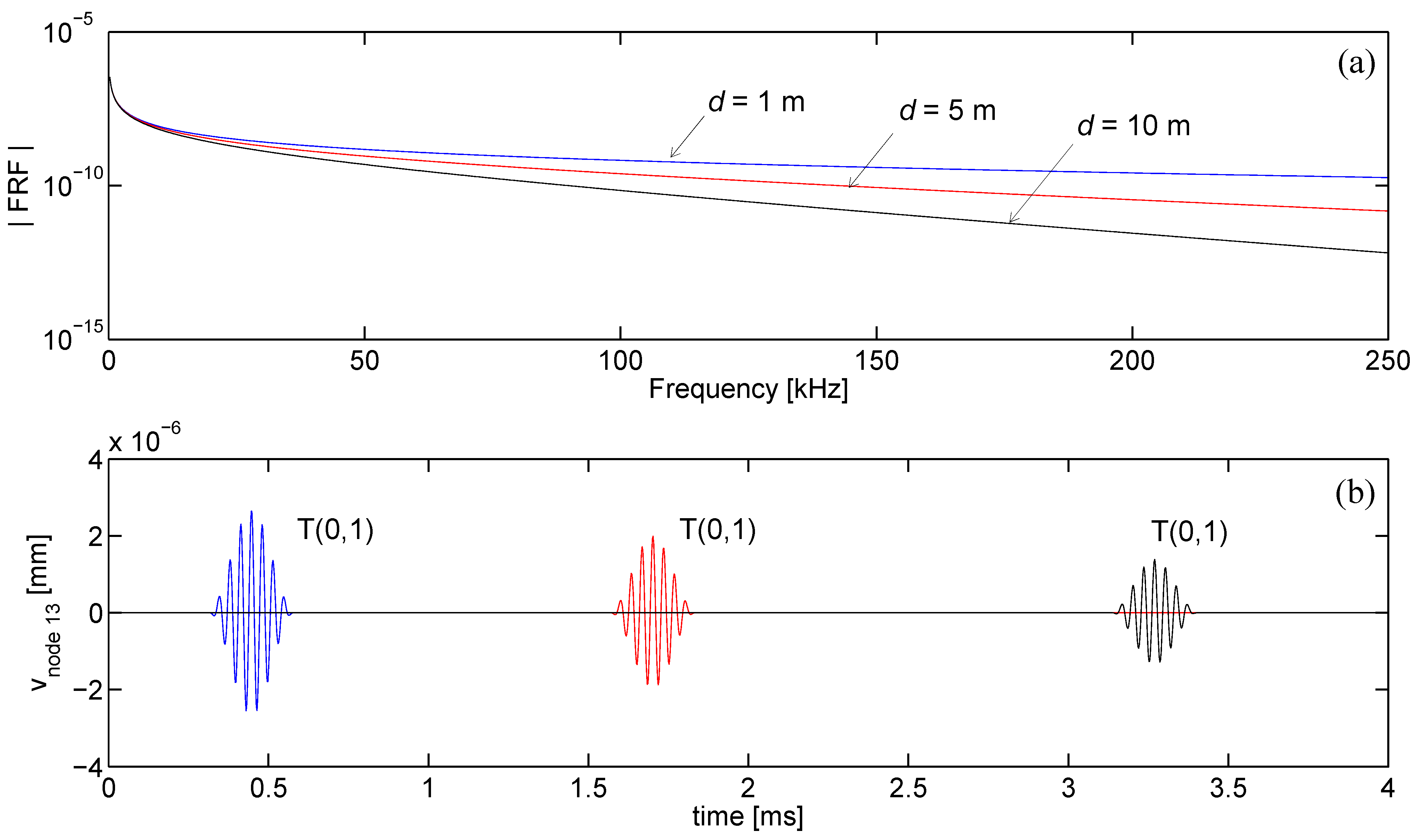
In this study an ad-hoc developed constant strain triangular (CST) finite element has been presented for calculating the three-dimensional time-transient response in a viscoelastic octagonal rod. The Hamilton’s principle has been used to formulate the weak form of the wave equation that is next transformed in the frequency domain. The major benefit of the frequency transformation comes from the possibility to easily account for linear viscoelastic constitutive relations. By solving a complex eigenvalue problem for a given wave frequency, wave equation roots are obtained in terms of complex wavenumbers, describing the spatial frequency and attenuation of the guided waves. A modal summation procedure and the application of the inverse time Fourier transform lead to the time-transient response of the problem for an applied time-dependent load.

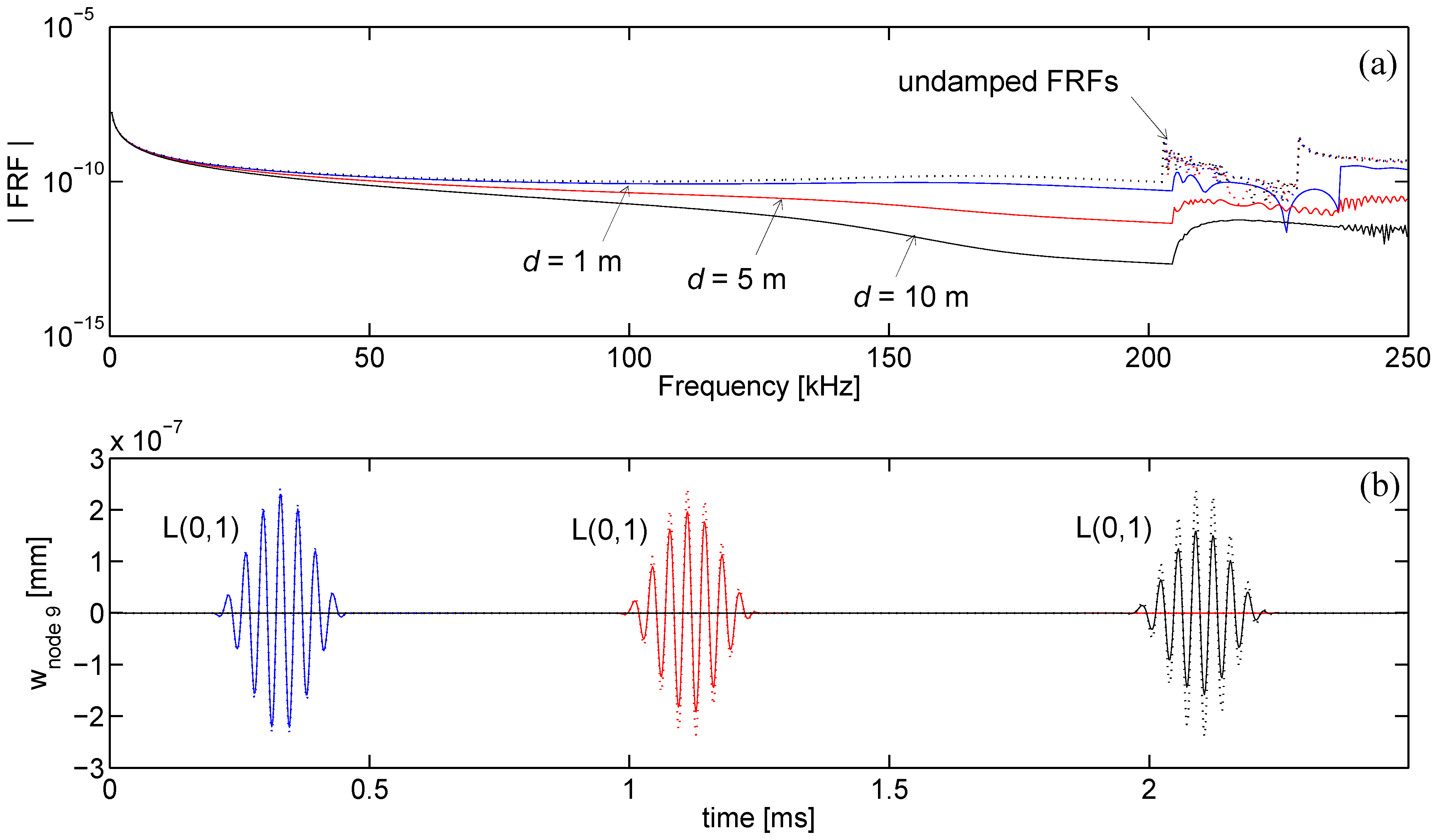
In the computation of the time-transient response, the proposed SFE formulation is reliable, capturing mode separation as well as pulse dispersion, stable, showing no or limited activity before the first arrival, and fast. The computational time mainly depends on the maximum excited frequency that sets the minimum number of finite elements in the mesh and the sampling frequency for which the waveguide frequency response [via Equation (29)] must be calculated to guarantee time-transient solution accuracy. For the proposed formulation the distance source-receiver only marginally affects the computational time and memory requirements, resulting advantageous if compared to a time transient Finite Element simulation for wave problems where an increased propagation distance involves a massive increase of dofs. This is particular true for high frequency computations, where the wavelengths are small and an accurate prediction by FE procedures involves an intensive three-dimensional discretization.

For example, the computation of each FRF and the corresponding time response required approximately 260 seconds using a Pentium 4 processor on a PC with 2 GB of RAM. This computational time is negligible if compared to the time needed by an equivalent full 3D Finite Element simulation to simulate waves at 10 meters distance.

In addition, SFE formulations allow for a very efficient multiple time-transient response calculation by means of an optimized post-processing procedure. In the time-transient response calculation, in fact, the majority of the computational CPU time is required to compute the waveguide eigenvalues and eigenvectors at several different frequencies solving the eigenvalue problem of Equation (18). The required time increases substantially for an increased number of dofs of the considered waveguide mesh. For a given waveguide, and especially for large dofs problems, wavenumbers and wavevectors can be calculated at the several different frequencies of interest only once and stored. Next, these data can be used to quickly calculate the time-transient response of the waveguide at the different dofs of the mesh, considering different distances source-receiver and also different spatial and temporal load distribution.

References and Notes

1. Liu, G.R.; Xi, Z.C. Elastic Waves in Anisotropic Laminates; 1st edition; CRC Press: Boca Raton, FL, USA, 2002. [Google Scholar]
2. Mukdadi, O.M.; Datta, S.K. Transient ultrasonic guided waves in layered plates with rectangular cross section. J. Appl. Phys. 2003, 93, 936–9370. [Google Scholar] [CrossRef]
3. Hayashi, T.; Song, W.J.; Rose, J.L. Guided wave dispersion curves for a bar with an arbitrary cross-section, a rod and rail example. Ultrasonics 2003, 41, 175–183. [Google Scholar] [CrossRef]
4. Bartoli, I.; Marzani, A.; di Scalea, L.F.; Viola, E. Modeling wave propagation in damped waveguides of arbitrary cross-section. J. Sound Vib. 2006, 295, 685–707. [Google Scholar] [CrossRef]
5. Marzani, A.; Viola, E.; Bartoli, I.; di Scalea, L.F.; Rizzo, P. A semi-analytical finite element formulation for modeling stress wave propagation in axisymmetric damped waveguides. J. Sound Vib. 2008, 308, 488–505. [Google Scholar] [CrossRef]
6. Treyssède, F. Elastic waves in helical waveguides. Wave motion 2007, 45, 457–470. [Google Scholar] [CrossRef]
7. Marzani, A. Time-transient response for ultrasonic guided waves propagating in damped cylinders. Int. J. Solids Struct. 2008, 45, 6347–6368. [Google Scholar] [CrossRef]
8. Loveday, P.W. Simulation of piezoelectric excitation of guided waves using waveguide finite elements. IEEE Trans. Ultrason. Ferroelectr. Freq. Control 2008, 55, 2038–45. [Google Scholar] [CrossRef] [PubMed]
9. Auld, B.A. Acoustic Fields and Waves in Solids (two volumes); 2th edition; Krieger Publishing Company: Malabar, FL, USA, 1990. [Google Scholar]
10. Damljanović, V.; Weaver, R.L. Forced response of a cylindrical waveguide with simulation of the wavenumber extraction problem. J. Acoust. Soc. Am. 2004, 115, 1582–1591. [Google Scholar] [CrossRef]
11. Biot, M.A. General theorems on the equivalence of group velocity and energy transport. Phys. Rev. 1957, 105, 1129–1137. [Google Scholar] [CrossRef]
12. Achenbach, J.D. Wave Propagation in Elastic Solids; North Holland Series in Applied Mathematics and Mechanics: Amsterdam, 1984. [Google Scholar]
13. Bernard, A.; Lowe, M.J.S.; Deschamps, M. Guided waves energy velocity in absorbing and non-absorbing plates. J. Acoust. Soc. Am. 2001, 110, 186–196. [Google Scholar] [CrossRef]
14. Galan, J.M.; Abascal, R. Numerical simulation of Lamb wave scattering in semi-finite plates. Int. J. Numer. Methods Eng. 2002, 53, 1145–1173. [Google Scholar] [CrossRef]