1. Introduction
Sensors allow computers to perceive the world that surrounds them. By the use of sensors, like thermostats or photocells, computers can meassure the temperature or lighting conditions of a room. In the last years,the deployment of multisensor networks has become popular due to the cut down on sensor prizes. This networks can include different kind of sensors, maybe more complex, like cameras, indoor location systems (ILS), microphones, etc …By the use of sensor networks computer systems can take more accurate decissions due to the richer information about the environment that they have.
A common task in sensor processing is the recognition of situations in the environment perceived. If these situations to recognize are known a priori, i.e. there is a set of labels that describe each situation, the problem can be tackled as a classification task. Then, the problem to solve is to find a model relating the data from sensor readings with situation labels. Some sensor data may be too noisy, and other not provide any information for label prediction. Relevant sensor data has to be identified to build the model from them, not including irrelevant data.
An application where the use of sensor networks can be useful is Human Activity Recognition, i.e., the understanding by the computer of what humans are doing. This field has received increasing attention in the last years, due to their promising applications that have in surveillance, human computer interaction or ambient intelligence, and the interests that governments and commercial organizations have placed in the area. Human Activity Recognition systems can be integrated with existing systems as the proposed by Corchado
et al. [
1] to monitor alzehimer patients. If a patient falls to the floor, the system can alert a nurse to attend the accident. Human Activity Recognition systems can also be integrated with the system proposed by Pavón
et al. [
2], detecting forbidden activities being performed and alerting security staff.
Human activity recognition may be considered as a classification task, and human activity recognizers can be created using supervised learning. A set of activities to recognized has to be defined a priori. Different observations about the activities to recognize are extracted using different sensors. Then, the problem to solve is to find the function that best relates observations to activity labels. Data from sensors is not free from noise, so relevant attributes have to be identified before training the activity recognizer. Better results are expected to be obtained when this previous step is performed.
The sensors that provides the most information for Human Activity Recognition are video cameras. Works in activity recognition from video could be divided in two groups [
3]: (1) those that are centered in small duration activities (i.e. walking, running,…); and (2) those that deal with large duration activities (i.e. leaving place, going to living room,…). The former are centered in choosing good features for activity recognition, whereas the latter usually tackle the temporal structure in the classifier.
Regarding small duration activities, Neural networks, Neuro-fuzzy systems and C4.5 have been succesfully employed [
4]. Also, time delay neural networks have been used to recognize the case where the activities are hand gestures [
5]. In [
6] is shown how to perform feature extraction, feature selection and classification using a simple bayesian classifier to solve the small duration activity recognition problem. In their approach, they use ground truth data from CAVIAR
* dataset of people bounding boxes instead of a blob tracker output. Perez
et al. [
7] use different time averaged speed measures to classify the activities present in the CAVIAR dataset using HMM.
Robertson
et al. [
3] uses trajectory and velocity concatenated data for five frames, and blob optical flow, to decide what is the current small duration activity. This small duration activity is then introduced in a Hidden Markov Model (HMM) to decide which is the small duration activity performed.
To classify large duration activities, Brand
et al. [
8] have used HMMs for modelling activities performed in an office. They use different spatial meassures taken from the blob bounding ellipse.The HMM approach has been extended in [
9] to model activities involving two agents, using a Coupled-HMM. They use different velocity meassures as features, being all of them invariant with respect to camera rotations and translations, providing camera independent recognizers.
HMMs are recognized as one effective technique for activity classification, because they offer dynamic time warping, have clear bayesian semantics and well-understood training algorithms. In this paper a method to adapt them, selecting the best features in the observation space, is defined, trying to maximize its accuracy for classifying short durative activities. HMMs will be incrementally built using both heuristic search and genetic algorithms. A comparative of the performance obtained using these algorithm for HMM construction will be shown. Our approach differs from the proposed by Ribeiro et al. in some aspects: (1) blob tracker output is used instead of ground truth data; (2) the foreground mask of the blob tracker is used to extract features; (3) the classifier used for the recognition of activities is an HMM; (4) we use different temporal window sizes; and (4) we use different search methods for feature selection.
This paper is organized as follows: on
section 2, an overview of the activity recognition system where the feature selection is going to be performed is given; on
section 3, the feature selection algorithms that are used to build HMMs are presented; on
section 4, experiments selecting good features for human activity recognition are performed and results are discussed; finally, on
section 5 conclusions of this work are presented and future lines are discused.
3. Feature selection for HMMs using Heuristic and Genetic Algorithms
Discriminant features have to be used in any classification problem to obtain good results. Also, HMMs have been widely used for activity classification, because activities can be easily represented using this abstraction. It seems to be of interest to study how HMMs could be built using feature selection techniques, because it is not clear that some commonly used features [
7] provide the necessary separability of the activities.
3.1. Feature subset evaluation
To evaluate the utility of a given feature subset an HMM
wrapper is going to be used. The utility of the feature subset will be the accuracy of the HMM for classifying some small duration activity sequences. Given a set of training sequences
,
containing
m different activities, and their corresponding set of hidden states
,
, the estimation of HMM parameters is straightforward. The HMM will have
m hidden states, one per activity. To estimate he initial state probability distribution, the frequency of each state to be the first in each training sequence has to be computed. The state transition probability distribution is going to be computed using the frequency of each state transition along the training sequences. To simplify even more the estimation of parameters, the observation symbol robability distribution is supposed to be a single multivariate gaussian distribution. Other type of distributions, like Gaussian Mixtures or KDE [
17] can be used, but the construction of the HMM will be harder, and it is not important for the objective of this work. The parameters of each state emission distribution to be estimated are the mean and covariance matrices.
Once that the Hidden Markov Model has been estimated, a test sequence can be classified using Viterbi Algorithm. The obtained state sequence is compared to ground truth data, and the accuracy of the model for predicting each hidden state is taken as the subset utility.
3.2. Searching the feature space
Given a set of N features, the number of possible feature subsets to evaluate is . As N grows, the feature selection problem becomes intractable and exhaustive search methods become unpractical. To avoid this course of dimensionality, suboptimal search methods have to be employed. In this paper two different methods are proposed: Best First Search and Genetic Search.
Best First Search (BFS) [
18] is a tree search method that explores the search tree expanding the best node at each level. In this case, the best node is the one who has the best accuracy on its level. Algorithm pseudocode is shown on 1. This search method does not guarantee to find the optimal solution, only a local optima, because when selecting only the best child, the path to the optimal solution could be left unexplored.
| Algorithm 1 Best First Search |
|
To search the feature subset space using Best First Search, the root node of the tree will be the empty feature set. The successors of a node will be that nodes that contain the same features that its parent plus a new one that its parent does not have. The search will finish were the accuracy of children is equal or smaller than the accuracy of their parent.
Genetic Algorithms (GA) [
19] are powerful search techniques inspired in the Darwinian Evolution Theory. Populations of individuals, where each one represents a different solution to the problem, are evolved using crossover and mutation operators. The pseudocode of a simple genetic algorithm can be seen on 2. Again, this search method does not guarantee to find the optimal solution, and even if it is found, there is no way to ensure that is the optimum.
| Algorithm 2 Genetic Algorithm |
while stop condition is not satisfied do end while
|
The individual that is going to be used to explore the feature subset space is a bit string of length N, being N the total number of given features. If the ith bit is set to 1, it means that the ith feature is selected, whereas if it is set to 0, it means that the ith feature is not selected.
4. Experimental validation
4.1. Experimental setup
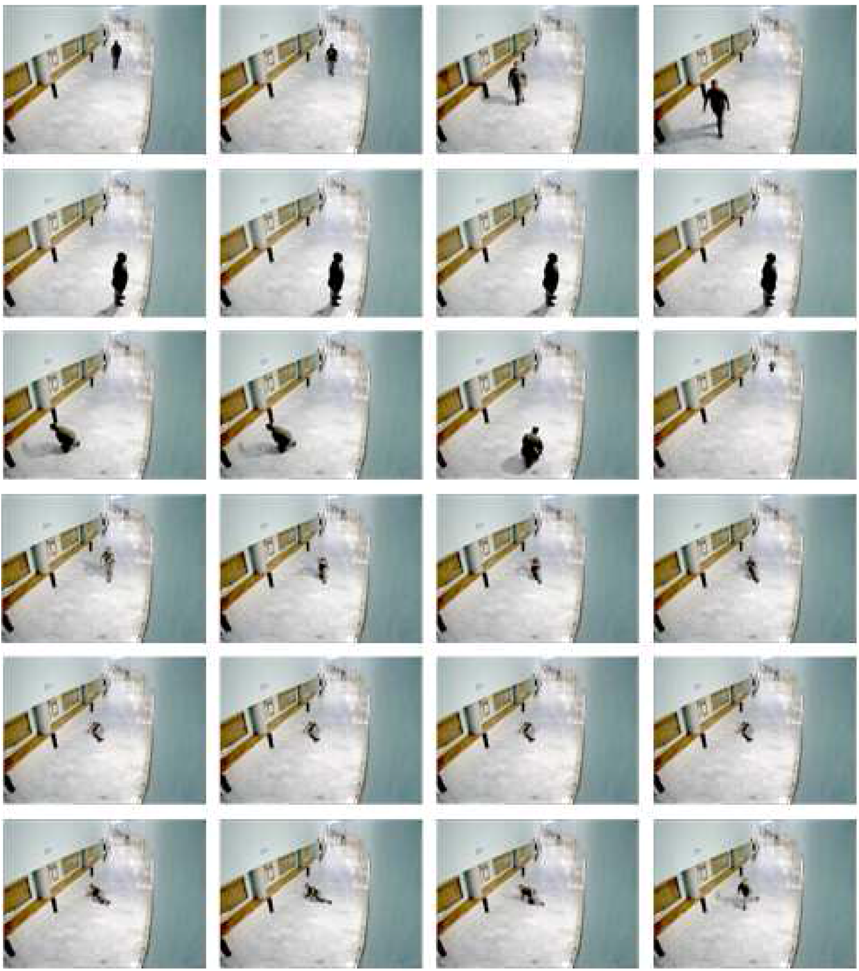
A video has been recorded at 25 fps on a corridor using a Sony SSC-DC598P video surveillance camera located about 3 meters from the ground. An actor has performed six different small duration activities:
walking,
stopped,
bending,
falling,
lied down and
rising (see
Figure 4). A blob tracker has been used to extract the actor bounding box on each frame where the actor appears. Using the bounding box, all the features presented on
section 2.2. have been extracted, using temporal windows from 3 to 25 frames, giving 780 different features per frame. The blob tracker has divided the original video on 11 video sequences where the activity being performed on each frame has been manually annotated. The content of each sequence could be seen on
Table 3.
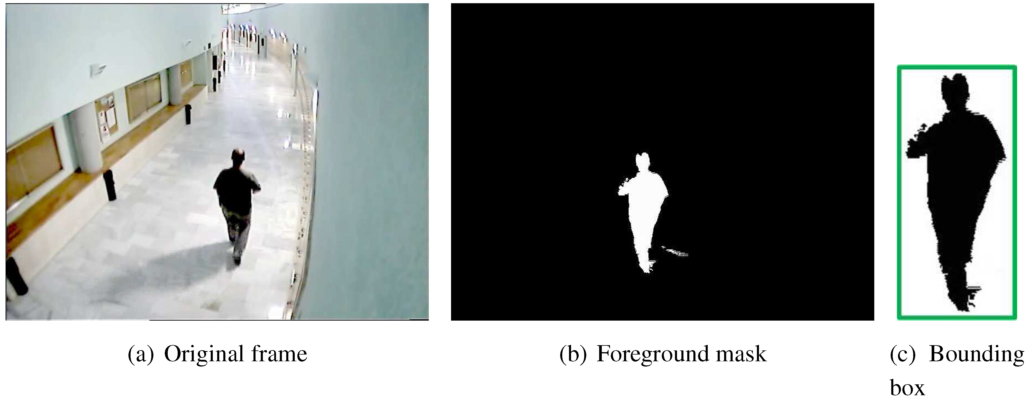
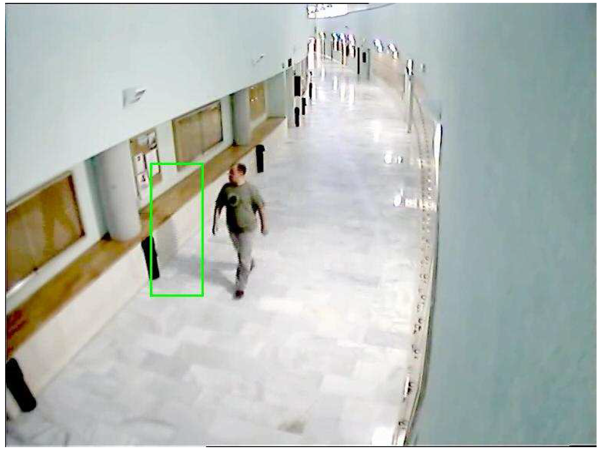
The blob tracker has produced some erroneous outputs, where the bounding box does not contain the actor for some frames (see
Figure 5. These errors may be produced by scene illumination changes, or by the initialization of a false track that is associated to the actor later. In this cases, the frame has been annotated with the especial activity
error. It has been considered that is important to have that label to be able to detect these type of false alarms when the system is working.
An HMM is going to be build for each set of small duration activities to be recognized using both BFS and GA. To evaluate the utility of a candidate feature subset, leave-one-out cross-validation (LOOCV) of the generated HMM is going to be performed with the sequences to be employed on each experiment. LOOCV consist on generate the model with all the sequences unless one and test the model with that sequence. This process is repeated for every sequence to be employed. Using this training strategy, possible overfittings are minimized, because the model has not been built with the sequence used to meassure its quality.
Figure 4.
Examples of the activities to recognize. First row, walking. Second row, stopped. Third row, lowing. Fourth row, falling. Fifth row, lied down. Last row, rising
Figure 4.
Examples of the activities to recognize. First row, walking. Second row, stopped. Third row, lowing. Fourth row, falling. Fifth row, lied down. Last row, rising
Table 3.
Content of the sequences used. W stands for walking, S for stopped, F for falling, D for lyed down, R for rising, L for bending and E for error. The number of frames that the activity last is shown between parenthesis
Table 3.
Content of the sequences used. W stands for walking, S for stopped, F for falling, D for lyed down, R for rising, L for bending and E for error. The number of frames that the activity last is shown between parenthesis
| Sequence | Content |
| 1 | W(220), S(214), W(113), E(197), S(161), W(221) |
| 2 | W(107), S(172), W(116), S(268), W(12) |
| 3 | W(50), S(134), W(112), S(202), W(224), S(181), W(145), S(239), E(5), S(30), W(269), S(190), W(250), E(55) |
| 4 | W(56), S(131), W(215), F(27), D(211), R(64), W(174), F(57), D(171), R(97), W(115), S(69), W(156), F(68), D(58), R(61) |
| 5 | W(139), F(57), D(79), R(88), W(130), F(54), D(172), R(80), W(176), F(52), D(52), R(82), W(236), E(22) |
| 6 | L(281), W(283), L(208), W(213), L(173), W(156), L(168), W(167), E(23) |
| 7 | W(62), L(134), W(146), L(43), W(222), L(157), W(158), L(110), W(80), L(180), W(133), L(168), W(28), E(18) |
| 8 | W(733), E(10) |
| 9 | W(760), E(48) |
| 10 | E(155), W(271), E(307) |
| 11 | W(65), E(1) |
Figure 5.
Example of the error activity. Bounding box (in green) does not contain the actor.
Figure 5.
Example of the error activity. Bounding box (in green) does not contain the actor.
GA has been employed using a configuration of 780 individuals and a mutation rate of . The selection technique employed has been tournament selection of 3 individuals. The population of the genetic algorithm is initialized with one random gen set to true. As the length of the individual is 780 and the population 780, it is expected to have each bit set to true in the population at least one time. Population evolution has stopped when the fitness value of the best individual has been without changing for 10 generations. The algorithm has been run 20 times for each experiment, because GAs are random search techniques and different results may be achieved in different trials. The result shown is the best one found.
4.2. Experiment I: three activities
A first attempt to solve the problem will be done using a set of sequences containing sequences 1, 2 and 3. It contains three different activities:
stopped,
walking and
noise. Results obtained with GA and BFS can be seen on
Table 4. Relative confusion matrix for the solution obtained by BFS is shown on
Table 5 and relative confusion matrix of the solution obtained by GA is shown on
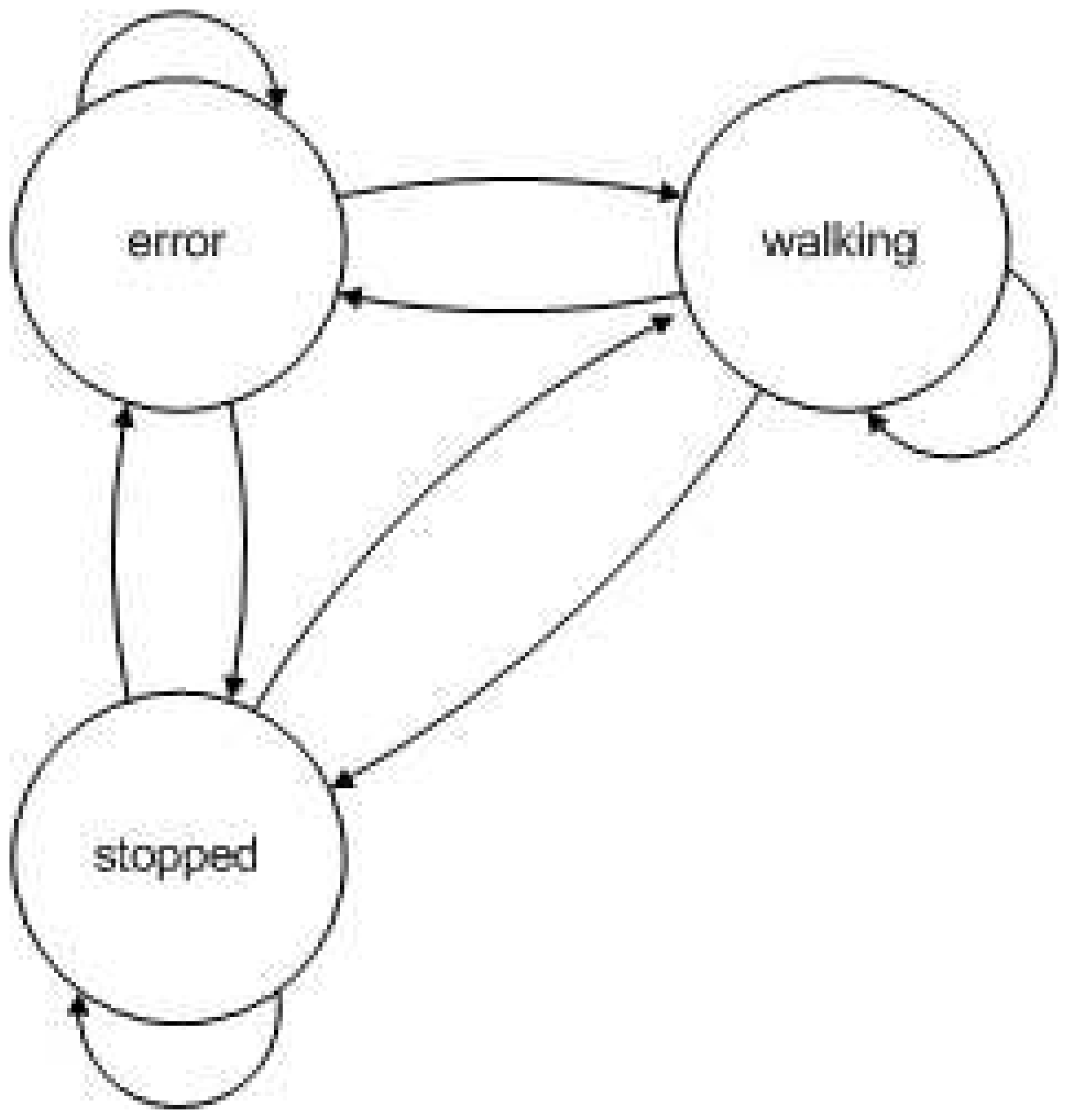
Table 6. Relative confusion matrices show the frequency of predicting errors per class. The HMM induced can be seen on
Figure 6
Table 4.
Features found by by Best First Search (BFS) and Genetic Algorithm(GA) for classificating three activities
Table 4.
Features found by by Best First Search (BFS) and Genetic Algorithm(GA) for classificating three activities
| Algorithm | Accuracy | Selection |
| BFS | 0.8699 | |
| GA | 0.9046 | |
The solution found by GA is better than the solution found by BFS according to the global accuracy. Also, taking a look in the confusion matrices of both classifiers (
Table 5 and
Table 6) reveals that the solution found by GA is better than the solution found by BFS for the accuracy of all the classes to predict. In both cases, the hardest class to predict is the
error class, maybe because it is the class with less examples.
Solution obtained by BFS algorithm includes different meassures of the optical flow. Solution obtained by GA includes velocity along y axes and different optical flow meassures.
Table 5.
Relative Confusion matrix for the HMM generated using BFS to classify the activities walking, stopped and error
Table 5.
Relative Confusion matrix for the HMM generated using BFS to classify the activities walking, stopped and error
| | prediction | error | walking | stopped |
| class | |
| error | 0.5869 | 0.4161 | 0 |
| walking | 0.0505 | 0.8984 | 0.0511 |
| stopped | 0.0531 | 0.0796 | 0.8673 |
Figure 6.
Structure of the HMM used in experiment 1
Figure 6.
Structure of the HMM used in experiment 1
Table 6.
Relative Confusion matrix for the HMM generated using GA to classify the activities walking, stopped and error
Table 6.
Relative Confusion matrix for the HMM generated using GA to classify the activities walking, stopped and error
| | prediction | error | walking | stopped |
| class | |
| error | 0.7521 | 0.0427 | 0.2051 |
| walking | 0.0238 | 0.9260 | 0.0502 |
| stopped | 0.0828 | 0.0251 | 0.8921 |
4.3. Experiment II: six activities
Two more sequences have been added to the set previously used: X and Y. Three new activities are going to be classified:
falling,
rising, and
lyed down. Results obtained with GA and BFS can be seen on
Table 7.
Table 7.
Features found by by Best First Search (BFS) and Genetic Algorithm(GA) for classificating six activities
Table 7.
Features found by by Best First Search (BFS) and Genetic Algorithm(GA) for classificating six activities
| Algorithm | Accuracy | Selection |
| BFS | 0.7051 | |
| GA | 0.7779 | |
Table 8.
Relative Confusion matrix for the HMM generated using BFS to classify the activities walking, stopped, falling, lyed down, rising and error
Table 8.
Relative Confusion matrix for the HMM generated using BFS to classify the activities walking, stopped, falling, lyed down, rising and error
| | prediction | error | walking | stopped | falling | lyed down | rising |
| class | |
| error | 0.2760 | 0.5082 | 0.0820 | 0.0984 | 0.0027 | 0.0328 |
| walking | 0.0098 | 0.8134 | 0.0225 | 0.0640 | 0.0060 | 0.0843 |
| stopped | 0.0050 | 0.1267 | 0.8092 | 0.0056 | 0.0195 | 0.0340 |
| falling | 0.0957 | 0.0319 | 0.0106 | 0.6596 | 0.2021 | 0 |
| lyed down | 0.0687 | 0.0102 | 0.3163 | 0.0037 | 0.5793 | 0.0219 |
| rising | 0.1588 | 0.5829 | 0.0118 | 0 | 0.0024 | 0.2441 |
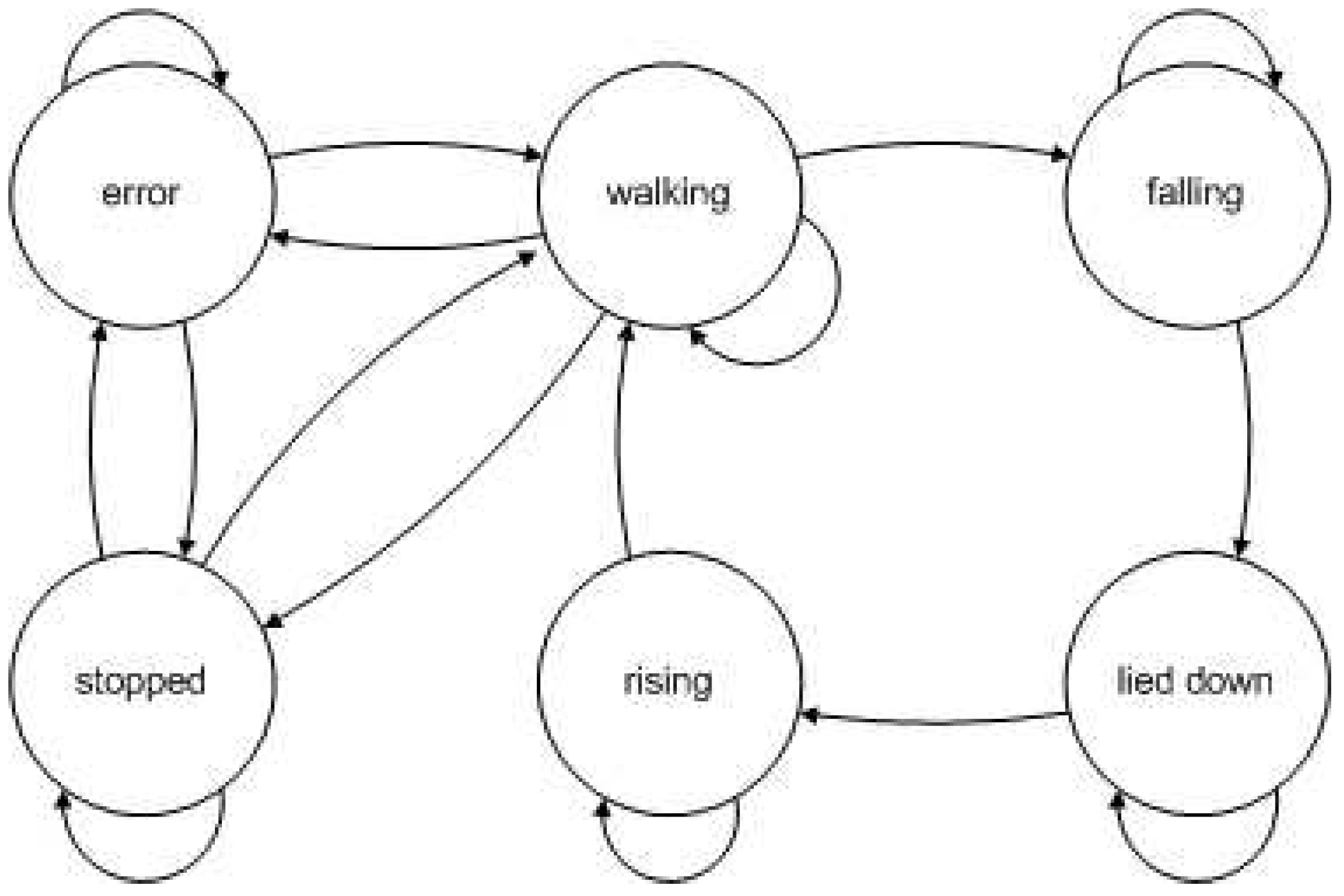
Figure 7.
Structure of the HMM used in experiment 2
Figure 7.
Structure of the HMM used in experiment 2
Again, the solution found by GA is better than the solution found by BFS if the global accuracy of the HMM induced (see
Figure 7 ) by the feature subset is considered. But now, taking a look into the
Table 9.
Relative Confusion matrix for the HMM generated using GA to classify the activities walking, stopped, falling, lyed down, rising and error
Table 9.
Relative Confusion matrix for the HMM generated using GA to classify the activities walking, stopped, falling, lyed down, rising and error
| | prediction | error | walking | stopped | falling | lyed down | rising |
| class | |
| error | 0.2509 | 0.5818 | 0.0982 | 0.04 | 0.0036 | 0.0255 |
| walking | 0.0163 | 0.8656 | 0.0291 | 0.0404 | 0.0041 | 0.0445 |
| stopped | 0.0671 | 0.0439 | 0.7803 | 0.0044 | 0.0623 | 0.0421 |
| falling | 0.0939 | 0.0712 | 0.0421 | 0.5243 | 0.1165 | 0.1521 |
| lyed down | 0.0012 | 0.0731 | 0.0899 | 0.0024 | 0.8046 | 0.0288 |
| rising | 0.0227 | 0.4434 | 0.0097 | 0.0032 | 0.0162 | 0.5049 |
confusion matrices of both classifiers (
Table 8 and
Table 9) reveals that the solution found by BFS is better for predicting classes
error,
stopped and
falling, while the solution found by GA is better for
walking,
lyed down and
rising.
Solution found by BFS includes optical flow and trajectory eccentricity meassures. GA includes also a shape descriptor.
Table 10.
Results obtained by Best First Search (BFS) and Genetic Algorithm(GA) using all the training sequences
Table 10.
Results obtained by Best First Search (BFS) and Genetic Algorithm(GA) using all the training sequences
| Algorithm | Accuracy | Selection |
| BFS | 0.7442 | |
| GA | 0.7501 | |
Table 11.
Relative Confusion matrix for de HMM generated using Best First Search
Table 11.
Relative Confusion matrix for de HMM generated using Best First Search
| | prediction | error | walking | bending | stopped | falling | lied down | rising |
| class | |
| error | 0.5514 | 0.1479 | 0.0210 | 0.1189 | 0.0040 | 0.0999 | 0.0569 |
| walking | 0.0111 | 0.8676 | 0.0603 | 0.0136 | 0.0118 | 0.0035 | 0.0320 |
| bending | 0.0318 | 0.3043 | 0.6304 | 0.0093 | 0.0039 | 0.0202 | 0 |
| stopped | 0.0606 | 0.0818 | 0.0596 | 0.7513 | 0.0139 | 0.0176 | 0.0153 |
| falling | 0.1293 | 0.2239 | 0.1139 | 0.0656 | 0.3301 | 0.0676 | 0.0695 |
| lied down | 0.0058 | 0.0361 | 0.2300 | 0.0926 | 0.0039 | 0.6218 | 0.0097 |
| rising | 0.0108 | 0.3459 | 0.1811 | 0.0405 | 0.0622 | 0.0216 | 0.3378 |
4.4. Experiment III: seven activities
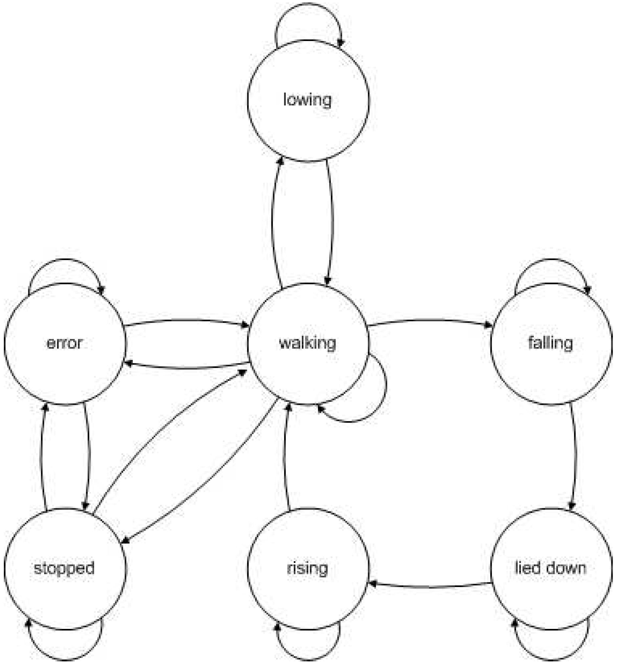
Finally, the eleven available sequences have been used to train the HMM models, adding a new activity to the previous experiment configurations:
bending (see HMM on
Figure 8). Results obtained with GA and BFS can be seen on
Table 10.
Table 12.
Relative Confusion matrix for de HMM generated using a Genetic Algorithm
Table 12.
Relative Confusion matrix for de HMM generated using a Genetic Algorithm
| | prediction | error | walking | bending | stopped | falling | lied down | rising |
| class | |
| error | 0.4881 | 0.1512 | 0.0148 | 0.1413 | 0.0267 | 0.1176 | 0.0603 |
| walking | 0.0101 | 0.8562 | 0.0701 | 0.0174 | 0.0166 | 0.0032 | 0.0264 |
| bending | 0.0196 | 0.2844 | 0.6815 | 0.0116 | 0.0029 | 0 | 0 |
| stopped | 0.0571 | 0.0421 | 0.0870 | 0.7758 | 0.0086 | 0.0122 | 0.0172 |
| falling | 0.0874 | 0.6053 | 0.0390 | 0.0031 | 0.2059 | 0.0265 | 0.0328 |
| lied down | 0.0692 | 0.0125 | 0.0999 | 0.0011 | 0.0170 | 0.7753 | 0.0250 |
| rising | 0.1486 | 0.2635 | 0.0203 | 0.0034 | 0.0304 | 0.0034 | 0.5304 |
Figure 8.
Structure of the HMM used in experiment 3
Figure 8.
Structure of the HMM used in experiment 3
Taking as the quality meassure the global accuracy of the HMM induced by the result subsets, the solution found by GA is a bit better than the solution found by BFS. According to cobfusion matrices of both classifiers (
Table 11 and
Table 12), solution found by BFS is better for predicting
falling and
error while the easiest are
walking and
stopped, whereas the solution found by GA is better for
bending,
stopped,
lied down and
rising.
Solutions found by both BFS and GA include shape descriptors and optical flow and trajectory eccentricity meassures.
4.5. Overall Discussion
Observing confusion matrices, it can be said that the activities performed on more frames are the best classified. That is due to the feature subset evaluation function used, that tries to maximize the global accuracy of the classifier. This effect can be avoided modifying the feature subset evaluation function to reward the correct classification of activities with fewer frames.
Solutions found by GA are smaller than the solutions found by BFS, so classification using the HMM generated by GA is easier than with the obtained by BFS. Besides classification cost, considering that the time needed to extract all the features is the same, extracting five features need less time than extracting nine, so the overall system using the solution by GA will be quicker. Also, the temporal window needed to extract the features found by GA tend to be smaller than for the features found by BFS (22 vs 11 frames), so the system using that feature set will have to store less information in its memory.


