Comparison of Different Neural Network Approaches for the Tropospheric Profiling over the Inter-tropical lands Using GPS Radio Occultation Data

Abstract

In this study different approaches based on multilayer perceptron neural networks are proposed and evaluated with the aim to retrieve tropospheric profiles by using GPS radio occultation data. We employed a data set of 445 occultations covering the land surface within the Tropics, split into desert and vegetation zone. The neural networks were trained with refractivity profiles as input computed from geometrical occultation parameters provided by the FORMOSAT-3/COSMIC satellites, while the targets were the dry and wet refractivity profiles and the dry pressure profiles obtained from the contemporary European Centre for Medium-Range Weather Forecast data. Such a new retrieval algorithm was chosen to solve the atmospheric profiling problem without the constraint of an independent knowledge of one atmospheric parameter at each GPS occultation.

1. Introduction

Global Positioning System (GPS) radio occultation (RO) is a global sounding technique for the atmospheric profiling useful for numerical weather models and climate studies. The RO technique employs GPS receivers placed on Low-Earth Orbit (LEO) satellites to sound the Earth’s atmosphere and ionosphere evaluating the additional delay affecting a radio signal when passing through the atmosphere due to the refractivity index variations [1].

This limb-sounding technique works under all-weather conditions due to the insensitivity of the GPS signal wavelength to scattering by clouds, aerosols, and precipitation, with a vertical resolution of about 1 km but a poor horizontal resolution (about 200 km).

Then, such GPS-LEO system is exploited to obtain profiles of refractivity, temperature, pressure and humidity in the atmosphere at global scale. Although the atmospheric refractivity profiling by radio occultation is a well-defined problem, care must be taken to compute temperature and particularly humidity profiles from refractivity [2]. In the troposphere, given an independent knowledge of temperature derived from independent observations (i.e. radiosoundings or data from atmospheric numerical modeling), GPS refractivity measurements are employed to derive water vapor partial pressure [3].

In this paper, we have proposed a new retrieval algorithm based on multilayer perceptron neural networks to derive profile of atmospheric parameters from RO refractivity profiles overcoming the requirement for temperature profile availability at each GPS occultation. In particular, we have implemented and compared different neural network trainings, employing three neural networks at each approach. The inputs are refractivity profiles computed from the occultation parameters observed by the COSMIC Microsat Constellation satellites and provided by the COSMIC Data Analysis and Archive Center (CDAAC) of Boulder (Colorado) [4]. The targets employed in the training are the dry and wet refractivity profiles, together with the dry pressure ones, obtained from the contemporary European Centre for Medium-Range Weather Forecast (ECMWF) analysis data.

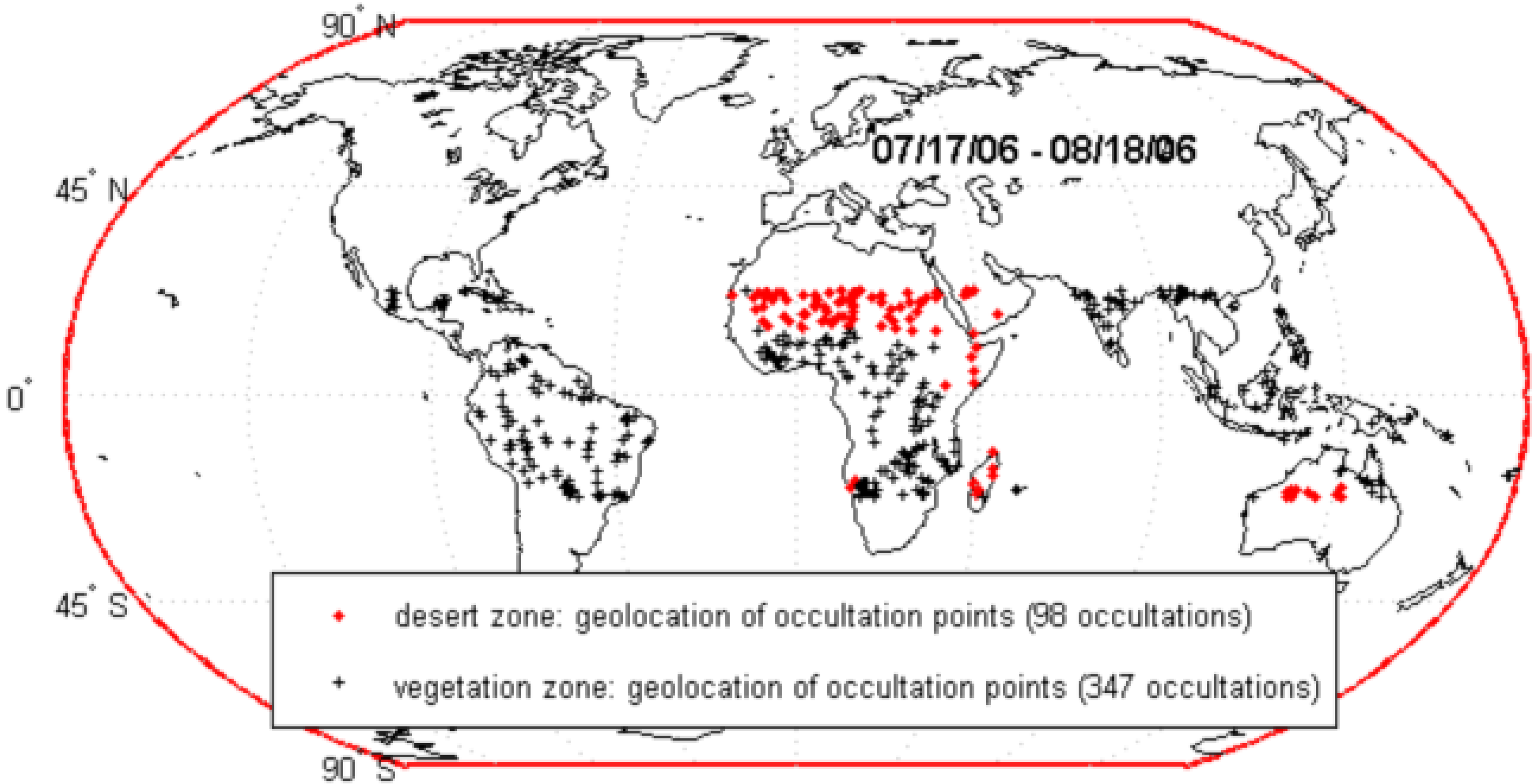
The neural network training and the following independent test were performed over the entire land area between Tropics, split into a desert and vegetation zone, by using the available data set of 445 refractivity profiles on summer 2006, from July 17 to August 18. The three networks estimating wet and dry refractivity and dry pressure allow us to obtain temperature and water vapor pressure profiles, without requiring independent information on atmospheric temperature.

The choice of splitting the entire available data set into desert and vegetation databases is to obtain three neural networks able to recognize homogeneous atmospheric conditions, since the humidity is affected by a large variability in the low troposphere, particularly.

To evaluate the performances of the different approaches, we have computed errors affecting the estimated profiles with respect to ECMWF analysis, assumed as the truth. Such a choice of ECMWF data as reference in the comparisons was also adopted by other authors [5,6], considering that these data provide global coverage and high spatial resolution reconstruction of the atmosphere.

The proposed algorithm shows the possibility to estimate tropospheric parameters included the wet ones only from RO refractivity, after the settlement of the training phase of neural networks, and hence the possibility to increase the atmospheric observations, thanks to a wide spatial coverage of RO soundings. For this purpose, the employment of neural networks proved useful and hence different training approaches were tested and evaluated not only from the standpoint of the retrieval accuracy, but also in terms of computational cost such as time and memory requirements.

2. Neural network input: profiles from radio occultation data

First, we have collected 445 FORMOSAT-3/COSMIC radio occultation events provided by CDAAC [7], covering the inter-tropical land area during the period from July 17 to August 18, 2006. The FORMOSAT-3/COSMIC is a joint Taiwan-U.S. mission of six micro-satellites, launched on April 2006, with onboard receivers registering phase and amplitude of radio waves at the two GPS carrier frequencies (1575.42 and 1227.6 MHz).

GPS radio signals passing through the atmosphere are refracted due to the vertical refractive profile: the overall effect of the atmosphere can be characterized by a total bending angle α, an asymptotic impact parameter a and a tangent radius r_p [2]. With the assumption of local spherical symmetry, the refraction index profile n can be retrieved from measurements of α as a function of a during an occultation by using an Abel transformation as in [8]:

$$n(r_p)=exp\left(\frac{1}{\pi }{\displaystyle \underset{a_{r_p}}{\overset{\infty }{\int }}\frac{\alpha (a)}{\sqrt{a^2-a_{r_p}^2}}da}\right)$$

(1)

where a_rp = n(r_p) · r_p is the impact parameter for the ray whose tangent radius is r_p. The refractivity profile is then N=(n-1) · 10⁶.

As a second step, we have computed the refractivity as in eq. (1) using the impact parameters and the bending angles profiles provided by CDAAC, vertically spaced from 4 m to 50 m in the low and high atmosphere, respectively.

The distribution of the considered GPS-RO events is shown in Figure 1. The FORMOSAT-3/COSMIC GPS occultations and the corresponding ECMWF observations have been co-located, in time and space, with a maximum time difference of 1 hour and a maximum geographical coordinate distance of 0.5°.

Figure 1. Distribution of FORMOSAT-3/COSMIC GPS occultation employed in the neural networks.

Figure 1. Distribution of FORMOSAT-3/COSMIC GPS occultation employed in the neural networks.

In order to train and test the neural networks we have created two uniform databases (desert and vegetation) of refractivity profiles sampled at the same altitude intervals for each RO observation. As a result, the desert database contains 98 profiles with 56 fixed altitude levels, representing the atmosphere from 1.1 to 12.1 km, i.e. the troposphere, and the vegetation database contains 347 profiles with 54 fixed altitude levels, representing the atmosphere from 1.4 to 12 km. Each profile is characterized by the vertical resolution of 200 m.

We have chosen RO with the minimum altitude of 1.1 km and 1.4 km over desert and vegetation area respectively as a trade-off between the requirement of a adequate number of observations to train the networks and the need of tropospheric profile estimation as much as possible close to the surface.

3. Neural network output: profiles from ECMWF data

The targets for the neural network training and the references for the following independent test are the dry and wet refractivity profiles and the dry pressure profiles. These profiles were obtained by processing data provided by the ECWMF belonging to the “ECMWF 91 model levels” data set, representing the atmosphere from 75 km to the ground with a vertical resolution spanning from 5 km to 25 m in the high and low atmosphere, respectively [9].

First, we have computed the water vapour partial pressure profile and then the dry pressure profile by subtracting the partial pressure of water vapor from the total pressure profile.

Hence, we have computed the atmospheric refractivity at microwave wavelength by [10]:

$$N=77.6\frac{P_d}{T}+72\frac{P_w}{T}+3.75\cdot {10}^5\frac{P_w}{T^2}$$

(2)

where P_d is the dry air pressure in mbar, P_w the water vapour partial pressure in mbar, T is the atmospheric temperature in Kelvin. Finally, we have vertically interpolated these profiles at the same altitude levels of the neural network input profiles.

In conclusion, the neural network outputs are the dry N_d and wet N_w refractivity profiles and the dry pressure profiles P_d, where N_d is:

$$N_d=77.6\frac{P_d}{T}$$

(3)

while N_w is the remaining part of eq. (2):

$$N_w=72\frac{P_w}{T}+3.75\cdot {10}^5\frac{P_w}{T^2}$$

(4)

The choice of these output profiles is justified as follows: to solve the atmospheric profiling problem, i.e. to retrieve T, P_d and P_w given N, the additional constraints of ideal gas and hydrostatic equilibrium laws are conventionally used in literature [2], [5]. Such an approach introduces another unknown, the air density ρ, leading to a system of three equations and four unknowns (T, P_d , P_w and ρ). Therefore it is necessary to have an independent knowledge of one of the four parameters to solve the atmospheric profiling problem [5], usually the temperature profile derived from independent observations or weather analysis [2]. Therefore, employing neural networks with inputs and outputs as described above, the atmospheric profile retrieval from refractivity can be solved using only eq. (2), overcoming the need of knowing the temperature profile at each GPS occultation.

Also, the networks act as a virtual equation describing the statistical information of the input and output data. It is worth noting that even if the GPS LEO retrieved refractivity profiles (input of the neural network) are affected by errors, the neural network outputs (dry and wet refractivity) are more consistent with the ECMWF profiles assumed as the truth, showing a kind of multivariate calibration ability of the trained networks.

In the next section, different training techniques will be proposed and compared to evaluate the neural network performances.

4. Tropospheric profiling with neural networks

As previously described, to solve the atmospheric profiling problem of GPS LEO occultations overcoming the need of external information, we have considered different neural network approaches for both desert and vegetation databases. For each database and each approach, we have trained three neural networks where predictors are the total refractivity profiles N computed from RO data using eq. (1), and the targets are the corresponding dry N_d and wet N_w refractivity profiles and the dry pressure profiles P_d computed from ECMWF data.

Over desert area between Tropics, the neural network training and the following independent test were performed by using 88 profiles for the training and the remaining 10 for the independent test, that represent 90% and 10% of the entire desert data set.

Over vegetation area between Tropics, we have proceeded in the same way by choosing 312 profiles for the training and the remaining 35 for the independent test.

First, before the training phase, we have pre-processed input and target features, with columns representing atmospheric parameter profiles, standardizing each row’s means to 0 and standard deviations to 1 [11]. After standardization, we have exploited different approaches for the neural networks learning, as described in the following section.

4.1 Early stopping technique

At first, we have applied the early stopping technique [11] to define the optimal number of training epochs for the training of the three neural networks. By using this technique, we have divided the available events in two disjoint subsets: the training set and the validation set. The first one is used for the learning itself, the second one to choose the number of training epochs. Learning ends when the error on the validation set begins to rise even if the error on the training set could be further reduced. In practice, the validation set improves the ability of generalization of the network. Since overtraining could occur even on the validation set, a further test subset should be used to assess the capacity of generalization of the network. Then we have divided the training desert data set (88 samples) and the training vegetation data set (312 samples) in three subsets respectively: the training subset used for the learning itself, the validation subset and the test subset, by assigning them randomly the 70% (62 and 218 samples for desert and vegetation lands respectively), the 15% (13 and 47 samples) and the 15% (13 and 47 samples) of the whole data sets, respectively.

Instead of the standard back-propagation, we have used the Levenberg-Marquardt optimization that is often the fastest back-propagation algorithm for training moderate-sized feed-forward neural networks, in agreement with the early stopping technique [12,13].

4.2 Early stopping technique with Principal Component Analysis

In the second approach, we have applied the same early stopping technique as described above, with the same division of the available data set, but we have processed the input and target matrices by the Principal Component Analysis (PCA). The PCA decomposes the 56-level and 54-level profiles, for desert and vegetation area respectively, on a basis of empirical orthogonal functions called principal components [14]. The PCA permits a reduction of the number of descriptive profile levels by exploiting the correlation among values at different altitudes, ensuring a faster processing and a reduction of computer memory requirements in comparison with the original data (full profiles). We have chosen to employ a number of principal components representing the 99.9% of the total variance of the original data [11], leading to the use of only 15 and 14 principal components for the total refractivity instead of the original 56 and 54 levels, over desert and vegetation lands respectively. Concerning the neural network targets, the number of components for dry refractivity, wet refractivity and dry pressure profiles are 11, 14 and 8 for the desert area. The need of a bigger number of wet refractivity principal components with respect to dry refractivity and dry pressure is an evidence of a greater variability in the troposphere of the wet parameters with respect to the dry ones, particularly over desert zones with respect to vegetation ones. In fact, concerning the neural network targets of the vegetation area, the number of components for dry and wet refractivity and dry pressure profiles are 11, 11 and 7 respectively, maybe sign of the perseverance of wet conditions over these sub-tropical zones, mainly for those ones closest to the equator.

4.3 Cross validation technique

Finally, we have applied the cross validation technique, together with the early stopping, useful in the case the available data set contains few profiles for training and testing neural networks. We have decided to use this approach for the shortage of profiles belonging to the desert data sets. Cross validation technique consists in dividing the whole considered data set in K subsets by training the neural networks with the profiles belonging to K-1 subsets and validating them with the profiles of the remaining subset. This process recurs K times by changing the validation set every time. The percentage of profiles used to train the neural networks is 1-1/K and, in this way, all the profiles are used in the learning and validating phase in turn. The only drawback of this technique is the need to repeat the learning K times, increasing the computational costs. For this reason, only profiles reduced with the PCA technique were employed, so cutting down the overall time processing.

Therefore, we have trained the neural networks with the cross validation technique applying both K=4 and K=8, that is with a validation subset corresponding to 25% and 12.5% of training data set.

Then we have divided the training desert data set (88 samples) and the training vegetation data set (312 samples) in the training subset and in the validation subset by assigning them, for K=4, the 75% (66 and 234 samples for desert and vegetation lands respectively) and the 25% (22 and 78 samples) of the whole data sets. Similarly, for K=8, the 87.5% (77 and 273 samples for desert and vegetation lands respectively) and the 12.5% (11 and 39 samples) of data sets.

5. Choice of neural network architectures

For each technique, we have considered feed-forward neural networks having, besides the input layer, a number (1 to 3) of hidden layers with tan-sigmoid transfer functions and an output layer with linear transfer functions [11]. To select the most suitable architecture, we have used a growing technique adding 1 neuron in the first hidden layer at each training session, until a maximum of 20 neurons for each hidden layer. We have considered a maximum of 3 hidden layers, choosing among the possible combinations the architecture with the lower Root Mean Square (RMS) error computed comparing the network outputs of the test session with the corresponding ECMWF profiles, where the test session employs the profiles not used in the training phase (10 and 35 observations from desert and vegetation databases, respectively).

The best neural network topologies in terms of performance for the dry refractivity, wet refractivity and dry pressure retrieval are reported in Table 1 and in Table 2 for desert and vegetation area, respectively. The optimal number of training epochs is greater for the early stopping with full profiles (less than 20 epochs), decreasing to about a half applying the PCA and the cross validation.

Table 1. Best neural network topologies over desert zone obtained for each neural network approach: input, HL1, HL2, HL3 and output columns report the number of neurons for the input, hidden layer 1, hidden layer 2, hidden layer 3 and output, respectively. Each approach employs 3 neural networks, named N Dry (for dry refractivity estimation), N Wet (for wet refractivity estimation) and P Dry (for dry pressure estimation).

Desert zone
EARLY STOPPING - PCA
	Input	HL1	HL2	HL3	Output
N Dry	15	11	2	-	11
N Wet	15	15	15	9	14
P Dry	15	6	6	5	8
EARLY STOPPING – Full Profile
N Dry	56	10	10	2	56
N Wet	56	9	8	-	56
P Dry	56	19	15	-	56
CROSS VALIDATION (25%) - PCA
N Dry	15	20	20	18	11
N Wet	15	15	15	13	14
P Dry	15	19	8	-	8
CROSS VALIDATION (12.5%) - PCA
N Dry	15	7	4	-	11
N Wet	15	16	13	-	14
P Dry	15	6	6	3	8

Table 1. Best neural network topologies over desert zone obtained for each neural network approach: input, HL1, HL2, HL3 and output columns report the number of neurons for the input, hidden layer 1, hidden layer 2, hidden layer 3 and output, respectively. Each approach employs 3 neural networks, named N Dry (for dry refractivity estimation), N Wet (for wet refractivity estimation) and P Dry (for dry pressure estimation).

Desert zone
EARLY STOPPING - PCA
	Input	HL1	HL2	HL3	Output
N Dry	15	11	2	-	11
N Wet	15	15	15	9	14
P Dry	15	6	6	5	8
EARLY STOPPING – Full Profile
N Dry	56	10	10	2	56
N Wet	56	9	8	-	56
P Dry	56	19	15	-	56
CROSS VALIDATION (25%) - PCA
N Dry	15	20	20	18	11
N Wet	15	15	15	13	14
P Dry	15	19	8	-	8
CROSS VALIDATION (12.5%) - PCA
N Dry	15	7	4	-	11
N Wet	15	16	13	-	14
P Dry	15	6	6	3	8

Table 2. Best neural network topologies over vegetation zone obtained for each neural network approach: input, HL1, HL2, HL3 and output columns report the number of neurons for the input, hidden layer 1, hidden layer 2, hidden layer 3 and output, respectively. Each approach employs 3 neural networks, named N Dry (for dry refractivity estimation), N Wet (for wet refractivity estimation) and P Dry (for dry pressure estimation).

Vegetation zone
EARLY STOPPING - PCA
	Input	HL1	HL2	HL3	Output
N Dry	14	6	6	3	11
N Wet	14	12	8	-	11
P Dry	14	10	10	10	7
EARLY STOPPING – Full Profile
N Dry	54	15	8	-	54
N Wet	54	12	5	-	54
P Dry	54	10	10	10	54
CROSS VALIDATION (25%) - PCA
N Dry	14	10	10	3	11
N Wet	14	4	-	-	11
P Dry	14	13	13	9	7
CROSS VALIDATION (12.5%) - PCA
N Dry	14	17	9	-	11
N Wet	14	12	12	12	11
P Dry	14	13	11	-	7

Table 2. Best neural network topologies over vegetation zone obtained for each neural network approach: input, HL1, HL2, HL3 and output columns report the number of neurons for the input, hidden layer 1, hidden layer 2, hidden layer 3 and output, respectively. Each approach employs 3 neural networks, named N Dry (for dry refractivity estimation), N Wet (for wet refractivity estimation) and P Dry (for dry pressure estimation).

Vegetation zone
EARLY STOPPING - PCA
	Input	HL1	HL2	HL3	Output
N Dry	14	6	6	3	11
N Wet	14	12	8	-	11
P Dry	14	10	10	10	7
EARLY STOPPING – Full Profile
N Dry	54	15	8	-	54
N Wet	54	12	5	-	54
P Dry	54	10	10	10	54
CROSS VALIDATION (25%) - PCA
N Dry	14	10	10	3	11
N Wet	14	4	-	-	11
P Dry	14	13	13	9	7
CROSS VALIDATION (12.5%) - PCA
N Dry	14	17	9	-	11
N Wet	14	12	12	12	11
P Dry	14	13	11	-	7

6. Results

As a first assessment of the employed training approaches, the vertically averaged RMS error is evaluated comparing N obtained as output of the different neural network trainings (N=N_d+N_w), hereafter named as the autotest result, with the corresponding ECMWF profiles. Also, the vertically averaged RMS error of N computed from Abel transformation, i.e. the input of the networks, and the mean standard deviation of the entire ECMWF database are reported in Table 3 and in Table 4, for desert and vegetation zone respectively. The ECMWF standard deviation can be assumed as an index of the climatological variability of a given atmospheric parameter, than a good accuracy of a retrieval algorithm is obtained when its RMS error is clearly below it. From these tables, we deduce the good performances of the proposed approaches, with the cross validation technique (12.5%) exhibiting the best results.

Table 3. Desert zone: mean standard deviation of ECMWF refractivity N, vertically averaged RMS error of refractivity N from Abel transformation and vertically averaged RMS error of refractivity N as output of neural network autotest (88 events) using the different approaches. E.S.: Early Stopping; C.V.: Cross Validation. The best result is highlighted.

Desert zone
Mean standard deviation of N from ECMWF	Vertically averaged RMS error of N from Abel transformation	Output autotest (88 events): vertically averaged RMS errors of N (N-units)
		E.S PCA	E.S. Full Profile	C.V. (25%) PCA	C.V. (12.5%) PCA
6.20 N-units	5.33 N-units	4.08 N-units	3.80 N-units	3.91 N-units	2.70 N-units

Table 3. Desert zone: mean standard deviation of ECMWF refractivity N, vertically averaged RMS error of refractivity N from Abel transformation and vertically averaged RMS error of refractivity N as output of neural network autotest (88 events) using the different approaches. E.S.: Early Stopping; C.V.: Cross Validation. The best result is highlighted.

Desert zone
Mean standard deviation of N from ECMWF	Vertically averaged RMS error of N from Abel transformation	Output autotest (88 events): vertically averaged RMS errors of N (N-units)
		E.S PCA	E.S. Full Profile	C.V. (25%) PCA	C.V. (12.5%) PCA
6.20 N-units	5.33 N-units	4.08 N-units	3.80 N-units	3.91 N-units	2.70 N-units

Table 4. Vegetation zone: mean standard deviation of ECMWF refractivity N, vertically averaged RMS error of refractivity N from Abel transformation and vertically averaged RMS error of refractivity N as output of neural network autotest (312 events) using the different approaches. E.S.: Early Stopping; C.V.: Cross Validation. The best result is highlighted.

Vegetation zone
Mean standard deviation of N from ECMWF	Vertically averaged RMS error of N from Abel transformation	Output autotest (312 events): vertically averaged RMS errors of N (N-units)
		E.S. PCA	E.S. Full Profile	C.V. (25%) PCA	C.V. (12.5%) PCA
7.11 N-units	4.76 N-units	3.70 N-units	4.06 N-units	3.80 N-units	3.41 N-units

Table 4. Vegetation zone: mean standard deviation of ECMWF refractivity N, vertically averaged RMS error of refractivity N from Abel transformation and vertically averaged RMS error of refractivity N as output of neural network autotest (312 events) using the different approaches. E.S.: Early Stopping; C.V.: Cross Validation. The best result is highlighted.

Vegetation zone
Mean standard deviation of N from ECMWF	Vertically averaged RMS error of N from Abel transformation	Output autotest (312 events): vertically averaged RMS errors of N (N-units)
		E.S. PCA	E.S. Full Profile	C.V. (25%) PCA	C.V. (12.5%) PCA
7.11 N-units	4.76 N-units	3.70 N-units	4.06 N-units	3.80 N-units	3.41 N-units

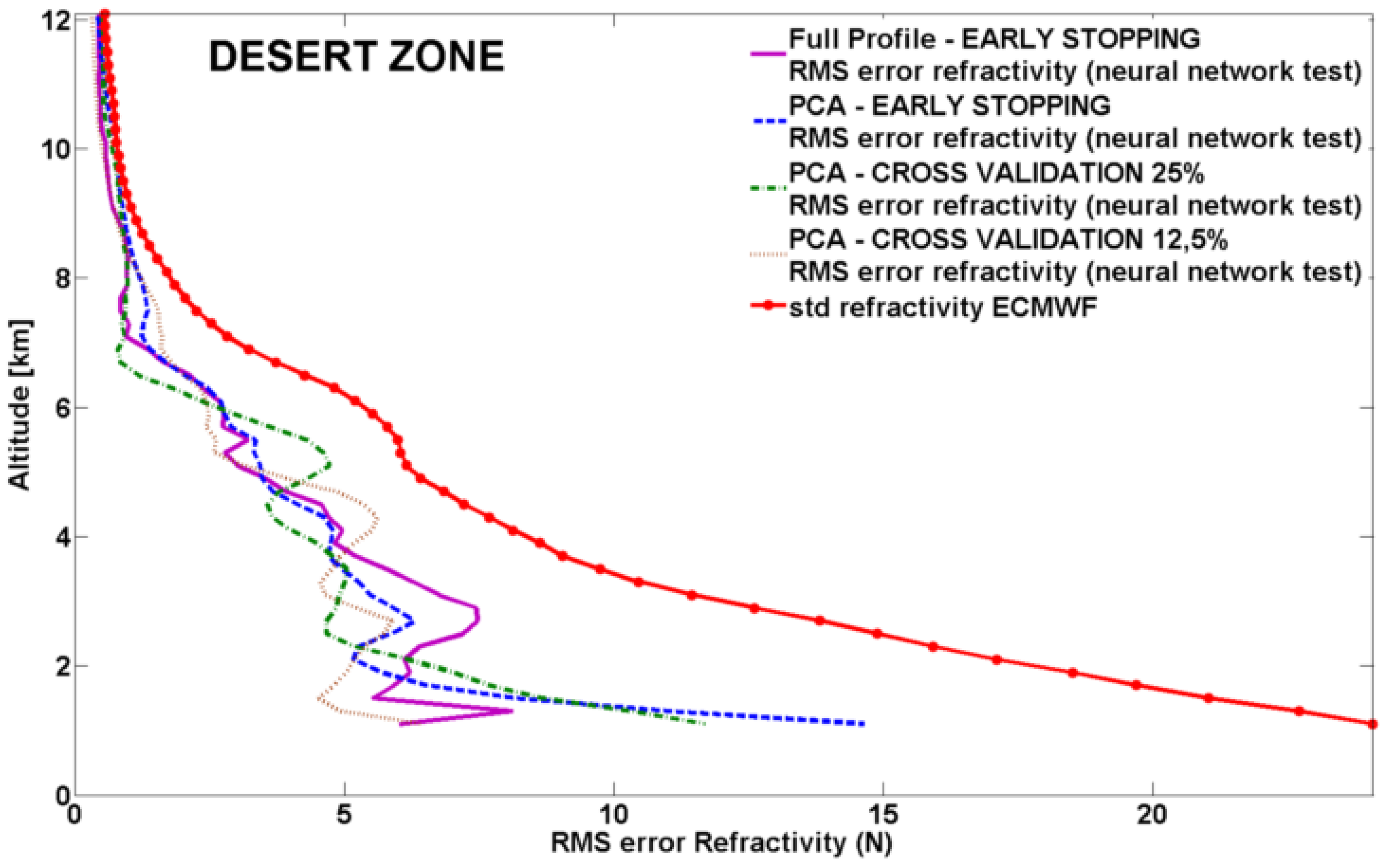
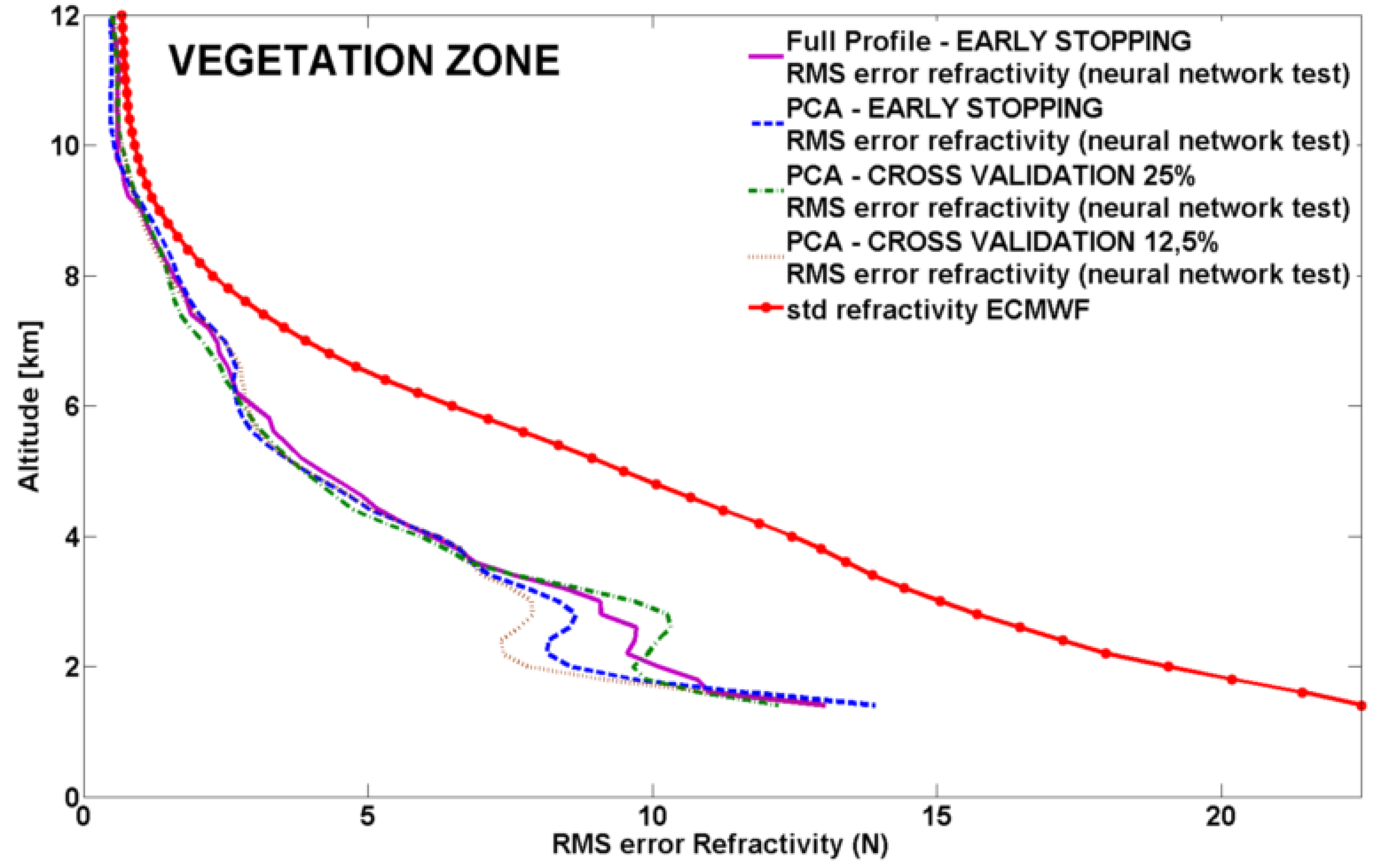
To evaluate performance and generalization capability of each neural network approach, the RMS error profiles for N (N=N_d+N_w) employing the independent test set of 10 and 35 occultations for desert and vegetation zones, are shown in Figure 2 and Figure 3, superimposed to the corresponding ECMWF standard deviation profiles.

Figure 2. Desert zone, neural network independent test (10 occultations): RMS error profiles for N using the different neural network approaches.

Figure 2. Desert zone, neural network independent test (10 occultations): RMS error profiles for N using the different neural network approaches.

Figure 3. Vegetation zone, neural network independent test (35 occultations): RMS error profiles for N using the different neural network approaches.

Figure 3. Vegetation zone, neural network independent test (35 occultations): RMS error profiles for N using the different neural network approaches.

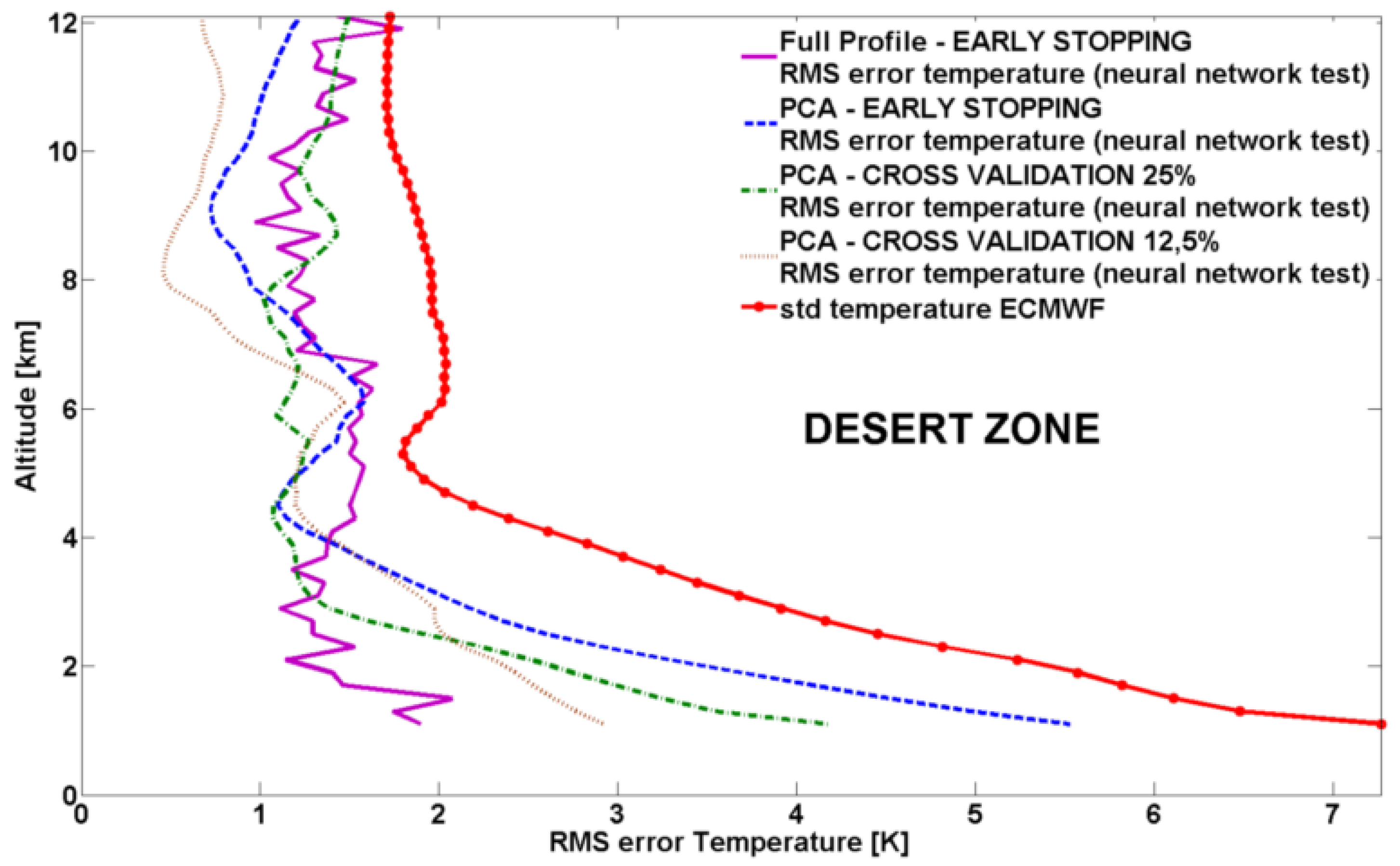
As underlined in the previous sections, choosing to train three networks for each approach enables us to retrieve atmospheric profiles without the constraint of temperature profile availability at each GPS occultation, only using eq. (2). In particular, with the availability of N_d, N_w and P_d, first we can solve for temperature T in a straightforward way from the dry refractivity using eq. (3), and then for partial pressure of water vapor P_w from the wet refractivity using eq. (4).

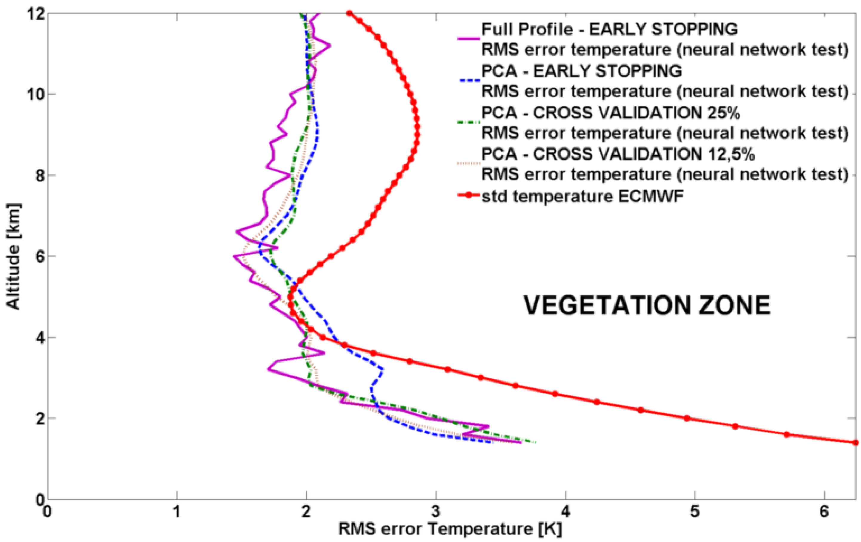
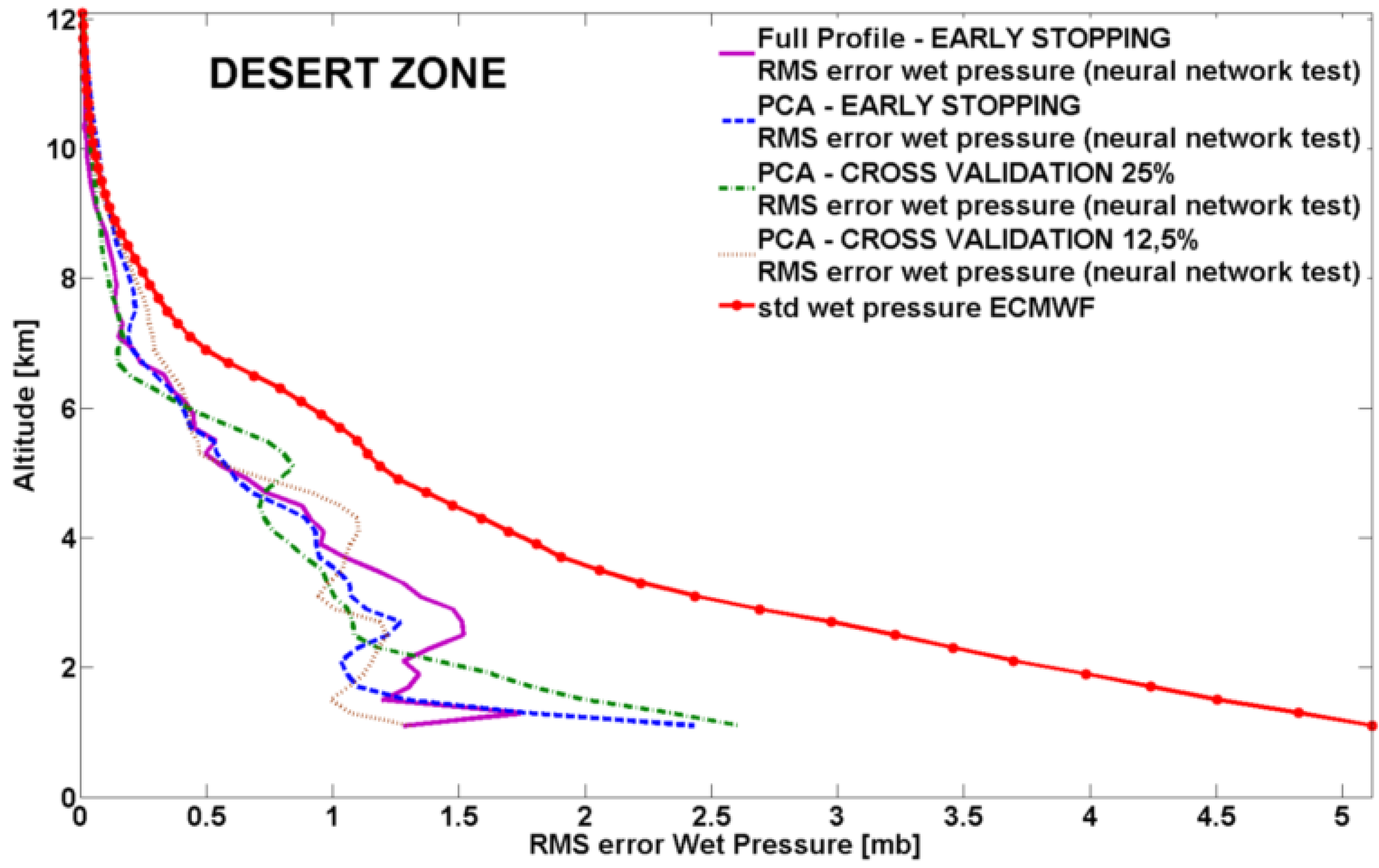
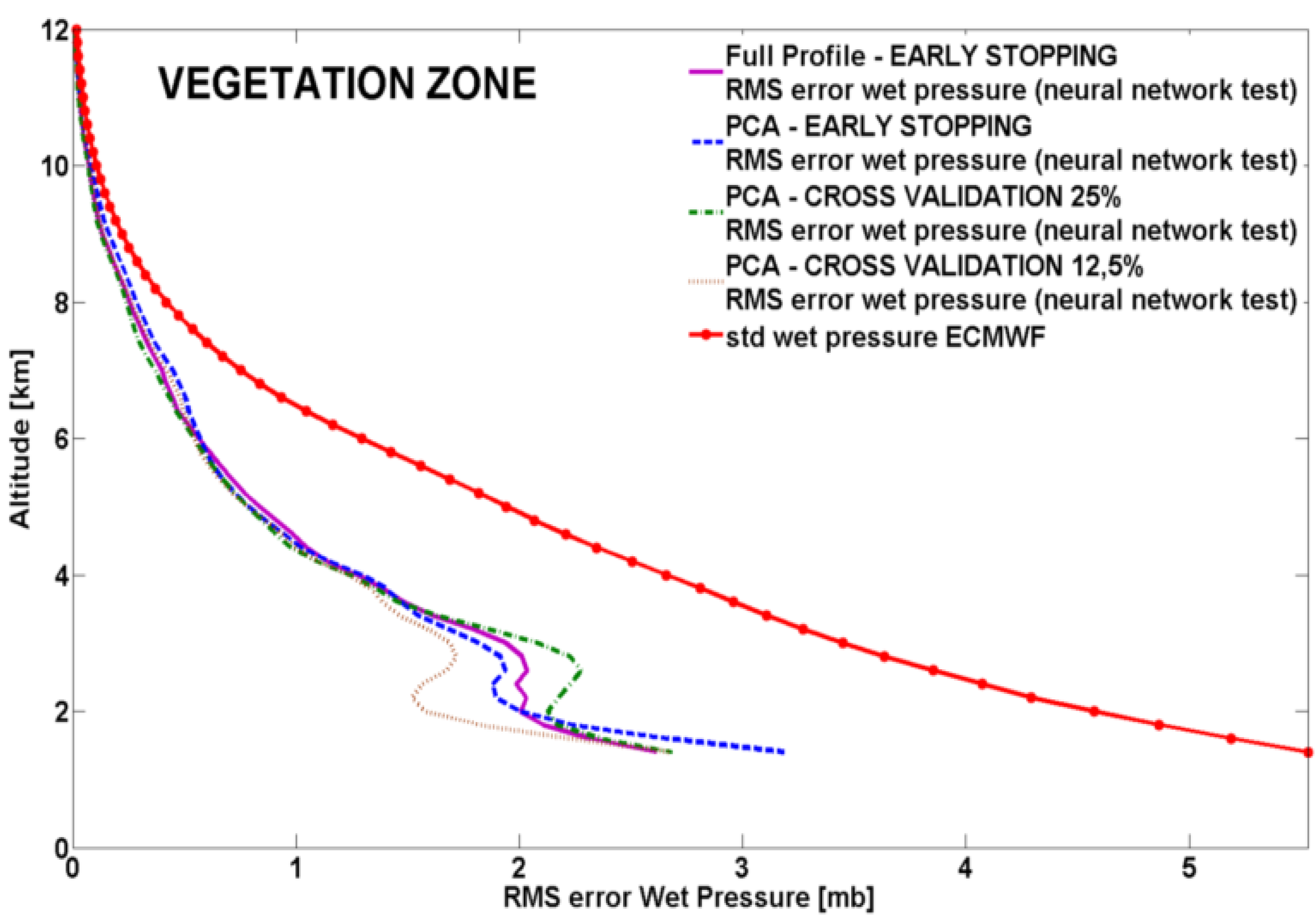
In Figure 4 and Figure 5 the RMS error profiles for T and in Figure 6 and Figure 7 the RMS error profiles for P_w are shown superimposed to the corresponding ECMWF standard deviation profiles, for desert and vegetation zone respectively.

Figure 4. Desert zone, neural network independent test (10 occultations): RMS error profiles for T using the different neural network approaches.

Figure 4. Desert zone, neural network independent test (10 occultations): RMS error profiles for T using the different neural network approaches.

Figure 5. Vegetation zone, neural network independent test (35 occultations): RMS error profiles for T using the different neural network approaches.

Figure 5. Vegetation zone, neural network independent test (35 occultations): RMS error profiles for T using the different neural network approaches.

Figure 6. Desert zone, neural network independent test (10 occultations): RMS error profiles for P_w using the different neural network approaches.

Figure 6. Desert zone, neural network independent test (10 occultations): RMS error profiles for P_w using the different neural network approaches.

Figure 7. Vegetation zone, neural network independent test (35 occultations): RMS error profiles for P_w using the different neural network approaches.

Figure 7. Vegetation zone, neural network independent test (35 occultations): RMS error profiles for P_w using the different neural network approaches.

In order to summarize the performances of each neural network approach on the ability to reconstruct all the analyzed tropospheric profiles, i.e. N_d, N_w, N, T, P_w and P (P=P_w+P_d), their vertically averaged RMS error values with respect to ECMWF data for the independent test are reported in Table 5 and Table 6. In the tables, the corresponding ECMWF mean standard deviations of the entire data set are also reported.

Analyzing the results, the ability of the neural networks to retrieve the atmospheric parameters is evident. By comparing the proposed approaches, it’s noticeable that each one produces good results, the best ones provided by using the early stopping with full profiles but especially by the cross validation with the PCA. Particularly, adequate accuracy is achieved in the lower troposphere over both the desert and vegetation zone, where the presence and the variability of the water vapour is more consistent. However, considering these approaches from the standpoint of the computational cost in terms of time and memory requirements, the cross validation with the PCA is less expensive than the only early stopping but with the full profiles.

7. Conclusion

In this work, we have proposed a method to estimate tropospheric profiles employing GPS RO observations over the entire land area between Tropics, during the summer time climatic conditions.

To overcome the necessity to know the true temperature profile at each occultation, we have trained three neural networks, by using different approaches, with targets permitting to solve the atmospheric profiling problem by using only RO data as input.

The results have shown globally good performances for each approach, especially if compared with the climatological variability of the data set. Moreover, neural networks trained with the cross validation technique exhibit good accuracy, where the use of profiles decomposed with the principal component analysis, i.e without preserving all the profile levels, ensures less expensive computational costs.

Table 5. Desert zone: mean standard deviation of ECMWF profiles, vertically averaged RMS error of dry refractivity (N Dry), wet refractivity (N Wet), total refractivity (N), dry pressure (P Dry), wet pressure (P Wet), total pressure (P) and temperature (T) profiles obtained by neural network independent test (10 events) using the different approaches. E.S.: Early Stopping; C.V.: Cross Validation. The best results are highlighted.

Desert zone
Parameters	ECMWF mean standard deviation	Output independent test (10 events): vertically averaged RMS error
		E.S. PCA	E.S. Full Profile	C.V. (25%) PCA	C.V. (12.5%) PCA
N Dry	1.52 N-units	0.94 N-units	0.74 N-units	0.86 N-units	0.79 N-units
N Wet	6.08 N-units	2.63 N-units	2.64 N-units	2.68 N-units	2.53 N-units
N	6.20 N-units	3.00 N-units	2.84 N-units	2.87 N-units	2.59 N-units
P Dry	2.44 mbar	1.42 mbar	1.42 mbar	1.12 mbar	1.21 mbar
P Wet	1.23 mbar	0.52 mbar	0.53 mbar	0.55 mbar	0.50 mbar
P	2.17 mbar	1.43 mbar	1.44 mbar	1.14 mbar	1.20 mbar
T	2.64 K	1.61 K	1.42 K	1.49 K	1.22 K

Table 5. Desert zone: mean standard deviation of ECMWF profiles, vertically averaged RMS error of dry refractivity (N Dry), wet refractivity (N Wet), total refractivity (N), dry pressure (P Dry), wet pressure (P Wet), total pressure (P) and temperature (T) profiles obtained by neural network independent test (10 events) using the different approaches. E.S.: Early Stopping; C.V.: Cross Validation. The best results are highlighted.

Desert zone
Parameters	ECMWF mean standard deviation	Output independent test (10 events): vertically averaged RMS error
		E.S. PCA	E.S. Full Profile	C.V. (25%) PCA	C.V. (12.5%) PCA
N Dry	1.52 N-units	0.94 N-units	0.74 N-units	0.86 N-units	0.79 N-units
N Wet	6.08 N-units	2.63 N-units	2.64 N-units	2.68 N-units	2.53 N-units
N	6.20 N-units	3.00 N-units	2.84 N-units	2.87 N-units	2.59 N-units
P Dry	2.44 mbar	1.42 mbar	1.42 mbar	1.12 mbar	1.21 mbar
P Wet	1.23 mbar	0.52 mbar	0.53 mbar	0.55 mbar	0.50 mbar
P	2.17 mbar	1.43 mbar	1.44 mbar	1.14 mbar	1.20 mbar
T	2.64 K	1.61 K	1.42 K	1.49 K	1.22 K

Table 6. Vegetation zone: comparison between mean standard deviation of ECMWF profiles, vertically averaged RMS error of dry refractivity (N Dry), wet refractivity (N Wet), refractivity (N), dry pressure (P Dry), wet pressure (P Wet), pressure (P) and temperature (T) profiles obtained by neural network independent test (35 events) using the different approaches. E.S.: Early Stopping; C.V.: Cross Validation. The best results are highlighted.

Vegetation zone
Parameters	ECMWF mean standard deviation	Output independent (35 events): vertically averaged RMS error
		E.S. PCA	E.S. Full Profile	C.V. (25%) PCA	C.V. (12.5%) PCA
N Dry	1.60 N-units	1.12 N-units	1.10 N-units	1.09 N-units	1.06 N-units
N Wet	7.75 N-units	3.83 N-units	3.82 N-units	3.81 N-units	3.51 N-units
N	7.11 N-units	3.64 N-units	3.81 N-units	3.74 N-units	3.53 N-units
P Dry	3.06 mbar	1.99 mbar	1.98 mbar	1.96 mbar	1.92 mbar
P Wet	1.54 mbar	0.76 mbar	0.74 mbar	0.75 mbar	0.68 mbar
P	2.49 mbar	1.86 mbar	1.82 mbar	1.77 mbar	1.82 mbar
T	2.85 K	2.12 K	1.97 K	2.08 K	2.02 K

Table 6. Vegetation zone: comparison between mean standard deviation of ECMWF profiles, vertically averaged RMS error of dry refractivity (N Dry), wet refractivity (N Wet), refractivity (N), dry pressure (P Dry), wet pressure (P Wet), pressure (P) and temperature (T) profiles obtained by neural network independent test (35 events) using the different approaches. E.S.: Early Stopping; C.V.: Cross Validation. The best results are highlighted.

Vegetation zone
Parameters	ECMWF mean standard deviation	Output independent (35 events): vertically averaged RMS error
		E.S. PCA	E.S. Full Profile	C.V. (25%) PCA	C.V. (12.5%) PCA
N Dry	1.60 N-units	1.12 N-units	1.10 N-units	1.09 N-units	1.06 N-units
N Wet	7.75 N-units	3.83 N-units	3.82 N-units	3.81 N-units	3.51 N-units
N	7.11 N-units	3.64 N-units	3.81 N-units	3.74 N-units	3.53 N-units
P Dry	3.06 mbar	1.99 mbar	1.98 mbar	1.96 mbar	1.92 mbar
P Wet	1.54 mbar	0.76 mbar	0.74 mbar	0.75 mbar	0.68 mbar
P	2.49 mbar	1.86 mbar	1.82 mbar	1.77 mbar	1.82 mbar
T	2.85 K	2.12 K	1.97 K	2.08 K	2.02 K