Algorithm for Active Suppression of Radiation and Acoustical Scattering Fields by Some Physical Bodies in Liquids

Abstract

An algorithm for the suppression of the radiation and scattering fields created by vibration of the smooth closed surface of a body of arbitrary shape placed in a liquid is designed and analytically explored. The frequency range of the suppression allows for both large and small wave sizes on the protected surface. An active control system is designed that consists of: (a) a subsystem for fast formation of a desired distribution of normal oscillatory velocities or displacements (on the basis of pulsed Huygens’ sources) and (b) a subsystem for catching and targeting of incident waves on the basis of a grid (one layer) of monopole microphones, surrounding the surface to be protected. The efficiency and stability of the control algorithm are considered. The algorithm forms the control signal during a time much smaller than the minimum time scale of the waves to be damped. The control algorithm includes logical and nonlinear operations, thus excluding interpretation of the control system as a traditional combination of linear electric circuits, where all parameters are constant (in time). This algorithm converts some physical body placed in a liquid into one that is transparent to a special class of incident waves. The active control system needs accurate information on its geometry, but does not need either prior or current information about the vibroacoustical characteristics of the protected surface, which in practical cases represents a vast amount of data.

1. Introduction

The presence of any body in a liquid is acoustically proclaimed by its radiation and scattering fields. The absence of these fields means that body is “acoustically invisible”. Invisible bodies are desirable in many cases, and this has led to numerous works devoted to the control of acoustical radiation and scattering fields created by bodies placed in liquids [1,2,3,4,5,6,7,8,9,10,11,12,13,14,15,16,20,21,22,24,25,26,27,28,29]. This problem is often divided into three subproblems: radiation suppression, suppression of backscattering, suppression of forward-scattering. It is always desirable to achieve effective suppression if: (1) the amount of available information about the boundary problem is minimum; (2) the amount of information about the incident waves is minimum; (3) the size of the suppressing sound system is minimum (for example, thickness of the protective coating, i.e., D_V/h>>1, λ/h >> 1, where D_V - body’s size, λ -length of the wave to be damped, h - coating thickness); (4) wide frequency range of the waves to be damped, i.e. ω_max/ω_min>>1 (where ω_max and ω_min are the maximum and minimum frequencies of the waves to be suppressed).

1.1. Passive Methods (Passive Coatings)

Passive methods to reduce the scattering field and radiating field require equipment of the protected body with some coating which uses wave absorption or interference, or a complicated coating based on metamaterials, but always without use of any outside source of energy.

Figure 1. Traditional thick passive coating for absorption (h>>λ) suppresses the body’s radiation and its back scattering, but does not suppress forward scattering (a); (cloaking [3,4,5,6,7]) thick (h>>λ) passive coating, constructed from metamaterials, makes the body transparent, but does not suppress the body’s radiation (b); thin (h<<λ) active coating, which suppresses both scattering to the back and forward scattering and radiation of the protected body. The horizontal parallel lines on the left side of (a-c) represent the power flux lines.

Figure 1. Traditional thick passive coating for absorption (h>>λ) suppresses the body’s radiation and its back scattering, but does not suppress forward scattering (a); (cloaking [3,4,5,6,7]) thick (h>>λ) passive coating, constructed from metamaterials, makes the body transparent, but does not suppress the body’s radiation (b); thin (h<<λ) active coating, which suppresses both scattering to the back and forward scattering and radiation of the protected body. The horizontal parallel lines on the left side of (a-c) represent the power flux lines.

1.1.1. Absorbing Coatings

Absorption by coatings can be effective if: (a) the external surface of the coating does (almost) not reflect the incident wave; (b) the incident wave, passing through the coating and reflected from the internal surface of the coating, becomes very weak (due to absorption) when returning to the external surface of coating. The main reasons to choose the such passive coatings are their simplicity, their wideband frequency range of incident waves and the wideband range of angles of incoming incident waves of arbitrary structures. Besides this, such coatings also suppress the radiation of the protected body (Figure 1a). The main drawback of passive coatings are their large thickness h (equivalent to several incident wavelengths λ>>h). This precludes the use of passive coatings in low frequency applications. Besides this, good absorbing coatings can only effectively suppress backscattering, but cannot suppress forward scattering.

Passive absorbing coatings can also be constructed from a large ensemble of passive oscillators with resonant absorption. In principle the thickness of such a coating can be much smaller than the length λ of the incident wave at a wide frequency band. However to absorb incident waves with oscillators, we need to compensate the dynamical interaction of oscillators, for instance, with special electroacoustical chains. In this case the parameters of each oscillator must depend on the arrival direction of each incident wave. This fact presents a great difficulty for effective absorption over a wide range of arrival directions, so a coating becomes very complicated oscillatory system, which is very sensitive to any small perturbation of its parameters. The body which does not produce backscattering and forward-scattering is called a "transparent body". We note again that absorbing coating reduces only back-scattering and creates a "black body", but does not reduce forwardscattering, and in principle cannot create a "transparent body".

Recently work devoted to a passive coating with distributed mechanical connections was published [2]. This coating has less thickness than a classic passive coating, but it reduces (at most) only back-scattering and does not suppress the radiation of the protected body.

1.1.2. Coatings Based on Interference

Multilayer interference coatings can have the thickness close to λ/4. However these coatings are effective only in the narrowband frequency range of incident waves and a narrow band of arrival directions. Interference coatings are used to scatter incident waves in some direction, unexpected by receiver systems (or in an unexpected frequency range).

1.1.3. Coatings Based on Metamaterials

Pendry and others [3,4,5,6,7,8] have provided several very attractive analytical solutions of the problem of transformation of any opaque body into a transparent one. These solutions are obtained with a ray-like representation of the wave fields both for electromagnetic and acoustical waves and are represented by a passive coating. This coating contains metamaterials (where, for instance, the phase and group velocities of a wave have mutually opposite signs). Due to the exotic characteristics of metamaterials, the incident wave avoids the protected body without scattering behind the body (see Figure 1b). For the solution by Pendry and others in its acoustical version [5] we need the anisotropic mass density, which is a difficult problem in practice. The drawbacks of this approach are: (a) the energy concentration of rays (and field intensity) in the tangential area of a coating with thickness h (Figure 1-b) becomes too large if D_V/h>>1;; (b) the thickness h of this coating must be much greater than the length λ of an incident wave (like in the passive absorptive coatings mentioned above) because the wave field is represented by rays; (c) this coating does not suppress any radiation from the protected body; (d) any practical realization of these coatings can achieve the desired exotic parameters only for sufficiently narrowband incident waves, due to the effects of the wave dispersion in the coating.

1.2. Active Methods

Active methods of sound control present an alternative to the passive ones and require an outside source of energy. The main difference between active and passive methods is the radiation of special waves, which have the same propagation direction and magnitude as the controlled waves, but the opposite wave sign. In the monochromatic case this means radiation of anti phase waves. Active methods can be attractive for the reason that active coatings can be of much thinner than the length of the wave to be damped (or an acoustically thin coating). To realize this coating we need very small sensors and actuators, electrically connected with the control center (computer). From a rigorous mathematical point of view, the methods for active control of waves represent a large branch of automatic control theory (or optimal control with criteria of minimum errors or fastest descent,…etc, see for instance the books by I. Lasiecka and others [17,18,19]).

1.2.1. Malyuzhinets’ Method

The possibility of controlling both radiation and scattering fields created by an arbitrary physical body (Figure 1c) was shown [25] by G.D. Malyuzhinets. This becomes possible due to the use of Huygens’ surfaces, characterized by unidirectional radiation (receipt). Practical implementation of this method requires the synthesis of Huygens’ radiating (and receiving) surfaces (with discrete elements) and development of the algorithm which connects them. The Malyuzhinets solution has been formulated for monochromatic fields. Practical solutions require causal algorithmic realization of this system in real time, wideband frequency range, and a spatially discrete form, which lead to great difficulties in a literal realization of Malyuzhinets’ theory. To realize Huygens’ surfaces, we need to use spatially discrete antenna arrays. The latter (and any devices required to attach them) must be acoustically transparent, i.e. the sizes of their elements and the spatial period of their spacing must be much smaller than the length of the waves to be suppressed. This is the reason why the magnitudes of the array’s elements must be much greater than the magnitude of the waves to be cancelled. On the other hand, to retain the unidirectional characteristics of the Huygens surface, the field of the discrete version of the Huygens surface (with addition of the reactive field) must be very small (this permits exclusion of their interaction with the protected body). This interaction could break the unidirectional characteristics of Huygens’ surfaces. This fact requires a permissible, but not very small distance between the array and the surface of a protected body. This creates a large technical difficulty: there is no way of placing a Huygens’ surface immediately on the surface of the protected body. Malyuzhinets’ theory has been tested experimentally and numerically for acoustical and electromagnetic waves [24,25,26,27,28,29].

1.2.2. Bobrovnitskii’s Active Method

Yu.I.Bobrovnitskii [20] has proposed a solution of the problem of an acoustically transparent (nonscattering) body as some expression of external active forces, which are applied to the protected surface, via full acoustical pressure, measured immediately on the protected surface, or via full oscillatory normal velocity, also measured immediately on this surface. The relation between measured and controlled values gives the active force for the compensation of a scattering field, i.e. converts the body into a transparent one. However under the conditions of a body’s neutral floatability in a liquid, active outside forces need mechanical support (i.e. a protected body), and these active forces induce additional oscillations of the protected body. These oscillations can be of very complicated shapes (in the case of a finite relation between elasticity of the body and compressibility of the external fluid) and of very simple shapes (in the case of oscillations of an ideally rigid body in a very compressible fluid). The scattering field can’t be suppressed without knowing these oscillations of the protected body, so we must simulate (by computer) the complicated vibroacoustical characteristics of the protected body very accurately, i.e. know all dynamic parameters of the body. To create the arbitrary desired force applied to body’s boundary we need either: (1) support for mechanical attachment (vibrostat); (2) or control of the body’s oscillations, based on full information about its dynamical behavior. In a lot of cases of practical interest the protected body has neutral floatability. This body is rigid, if it is surrounded by air, but this body is soft for acoustical pressure in a liquid. Vibroacoustical parameters of the body are characterized simultaneously: (1) by a vast volume of information; (2) by fast temporal changes of this information, due to temporal changes of temperature and hydrostatic pressure outside the protected body. This does not permit identification of a body’s parameters with sufficient quickness for effective control [23].

1.2.3. Joint Suppression of Radiating and Scattering Field by a Coating of Controlled Thickness

The algorithm of active coating thickness control to suppress radiation and scattering fields is described in [21]. This coating is interacting both with the protected body and the outside media. For control we need know the instant distributions of oscillatory normal velocity of the inside surface of the coating and the instant sound pressure on the outside surface of the coating. Besides this we must know all (and accurately) the vibroacoustical characteristics of the protected body in a vacuum [23]. In addtion, for the system stability these vibroacoustical characteristics must satisfy some conditions too. Thus, we must exclude interactions between the active system and the protected body. Again we consider Huygens’ sources and the modified approach of Maliuzhinets. The new approach allows quick suppression of scattering fields with minimum information about the boundary problem. The one-sided direction of the radiation of Huygens’ sources allows us to form the distribution of oscillatory velocities (or displacements), which we need, on the outside surface of an active coating, without inducing additional oscillations of the protected body [25,36,37]. At this point the analogy between Malyuzhinets’s method and our approach is over.

1.2.4. Rules of Chain Substitution

As the basis of the suggested approach, we took the way of fast tuning of normal velocity, its matching with incident waves: if the normal velocity of the external surface of a coating is identical with the projection of particle velocities (normal to the body surface ), caused by an incident wave in uniform media (i.e. in the absence of scattering bodies), then the scattered wave is absent. In this way we solve the problem of radiation suppression in the absence of incident waves: normal velocity of surface must be zero (and the radiation zero).

Figure 2. The half-infinite line of wave transmission (broken at the length L₀); i₀, u₀ -current and voltage (complex magnitudes) on the left end is induced by source ε₀ before cutting. i₁, u₁ - current and voltage (complex magnitudes) in the broken point before cutting. There are three equivalent boundary conditions (or substitutions) on the right hand end of the piece of transmission line (of length L₀), when the source ε₀ “does not feel” the difference between them and infinite (L₁ → ∞) line of transmission: active source of current i₁, active source of voltage u₁, passive impedance z₁ = u₁/i₁.

Figure 2. The half-infinite line of wave transmission (broken at the length L₀); i₀, u₀ -current and voltage (complex magnitudes) on the left end is induced by source ε₀ before cutting. i₁, u₁ - current and voltage (complex magnitudes) in the broken point before cutting. There are three equivalent boundary conditions (or substitutions) on the right hand end of the piece of transmission line (of length L₀), when the source ε₀ “does not feel” the difference between them and infinite (L₁ → ∞) line of transmission: active source of current i₁, active source of voltage u₁, passive impedance z₁ = u₁/i₁.

The approach, which is suggested below, can be explained by the simple example of changing of elements in oscillatory electric circuits, without changing currents (velocities) and voltages (forces) in electric or mechanical circuits. The acoustical analog of inserted (changed) elements is a transparent area in an infinite space, filled by the same homogeneous compressible liquid, but this area is planned to be filled by some protected body, which we must make transparent too, so the sources of external waves “would not” feel any difference in boundary problem. In the language of electrical oscillatory chains this operation (called “substitution”) means such a change of some chain element, which can’t be detected by the sources, so the sources of the external waves must not "feel" any additional influences, fulfilled by change of boundary problem. Of course we are not interested in the substitution, which is trivial and copies all the characteristics of changed elements. We are interested in the cases when "invisibility" of such change may be achieved with minimum tools: (a) satisfying the same (as before the substitution) electric voltage (force, pressure) in the break point of the active device; (b) satisfying the same (as before substitution) electric current (velocity) in the active device at the break point; (с) satisfying the same ratio between electric current (velocity) and electric voltage (force) (i.e. impedance as before substitution) (see [22]).

1.2.5. Choice of Velocity or Displacement Control (Nonequivalence of Velocity and Pressure Control)

In the problem, which was presented above, the substitution area does not radiate or scatter waves, so for electric and mechanical chains all three ways are equivalent. Let’s note also, that in the absence of tangential (viscosity) stresses in the external fluid matching of both normal velocities and matching of acoustical pressure are equivalent. This is due to the inevitable mutual connection between pressure and normal velocity on the protected surface S_V. Mathematically this means the existence of an operator (surface integral), due to which any distribution of normal velocities (on S_V) creates only one possible distribution of acoustical pressure on this surface S_V. On the other hand, we always can find the operator (surface integral), due to which any distribution of acoustical pressure (on S_V) creates the only possible distribution of pressure on this surface S_V. Thus we can’t create pressure and normal velocity fields independently. In the opposite case, after tuning the velocity is fulfilled, we will try to tune the pressure and inevitably must break the tuned velocity, achieved above (and analogously in the inverse direction). Below we have chosen the tuning of normal velocities, because the kinematic value - normal displacement of the controlled boundary has one very important characteristic: it remains (saved) after the end of short pressure pulse (blow), which created this displacement. Now we will describe the one-dimensional boundary problem, where a short blow (uniformly distributed along the plane border) induces normal displacement of the plane border of the elastic half-space (without any dissipation in material). Normal displacement, caused by blow, will remain constant (“frozen”) during an arbitrary unlimited time (Figure 3a). This effect can be interpreted as some plasticity of the plane boundary, separating the elastic half-space. On the other hand, a pressure pulse, which was created by the same blow, departs from the blow point with the speed c_w of sound propagation, so this boundary cannot save in memory the pressure pulse (caused by the same blow) after the termination of blow. The reason of this difference in behavior of wave fields (pressure and displacement) can be found on a micro level too, for example − in the acoustical monopole field: acoustical pressure p = p₀r^-1exp(–ikr + iωt), created by a monopole is proportional only to r^-1 (which describes radiation field), but the radial velocity field υ = (p₀/ρ_wc_w)[r^-1+(ik)^-1r^-2]exp(–ikr+iωt) of the monopole contains the term r^-2 (which describes the non-radiation field) besides the radiation term r^-1 (r - denotes the distance from monopole center to the watch point, ρ_w -mass density of media, c_w - speed of sound in compressible media, k = 2π/λ -wave number, λ -wavelength). To illustrate the difference between pressure control and velocity (displacement) a simple scenario is presented in Figure 3a,b. There the series of fast deformations ("instant photos") of a half-infinite elastic rod with square cross-section (Figure 3-a) and a half-infinite space filled with an elastic compressible medium (Figure 3b) at the moment t=0, 0<t₁<t₂<t₃<…after a blow by the same “hammer” (with same square shape of cross-section with dimension D_h x D_h and the same initial mechanical impulse) during the time τ_c <<D_h/c_w. So the hammer during the interval τ_c makes the rod shorter by the value A_h (Figure 3a) and makes an imprint of cross-section D_h x D_h and depth Ah=Jρ_w^-1/2E_w^-1/2D_v^-2 in the border of half infinite elastic space (Figure 3b). We suppose that all residual space in Figure 3 (besides the elastic rod and elastic half-space) is filled with vacuum. Above we denoted: J -mechanical impulse of hammer’s blow, ρ_w -mass density, E_w -Young’s modulus (Figure 3a) of the rod material and analogously for compressibility of a half space media (Figure 3b), c_w - speed of longitudinal sound propagation in the rod material and the elastic half-space. Life-time of rod’s shortening is ${\overline{\mathsf{\tau }}}_L=\infty$ (Figure 3-a). On the other hand the life-time of the imprint in the plane border of compressible half-space is τ_L ≈ D_h/c_w. We note that:

$${\mathsf{\tau }}_L>>{\mathsf{\tau }}_c$$

(1)

In Figure 3c the evolution of the following scenario is presented: the plane boundary of the infinite compressible half space is excited by a uniform bipolar (step-like) blow of pressure with a sign change in the point x = 0. During pressure blow time (0, τ_c) this pulse creates a step-like bipolar deformation (imprint) u(x,0,τ_c) of the boundary z = 0. After the blow the deformation becomes more smooth along with propagation (with velocity c ≤ c_w) in all tangential directions and will have a smaller step magnitude of (up to zero at |x| →∞). We note that at time interval (0, τ_c) this problem (as in Figure 3b) is fully one-dimensional (under condition (1)), but at times t > τ_c) the boundary problem becomes significantly two-dimensional (see Section 5.5 below).

Figure 3. On the nonequivalence of control of velocity and control of pressure: "plasticity" in the boundary problems without dissipation.

Figure 3. On the nonequivalence of control of velocity and control of pressure: "plasticity" in the boundary problems without dissipation.

2. Features of the Statement of the Problem

Below we search for the solution in the form of an active system with the following qualitative characteristics:

a)

simultaneous suppression of radiation and scattering fields of the protected body;

b)

wide frequency range of suppression;

c)

minimum prior and current information on the incident waves and radiation waves;

d)

minimum prior and current information on the vibroacoustical characteristics of protected body;

c)

neutral floatability of protected body in liquid;

d)

quick response of active system, caused by changes of the incident wave field.

The protected body is of neutral floatability and can be both much larger and much smaller than the length of wave to be suppressed. Parameters of the protected body are unknown, but its shape is smooth, closed and convex (we assume the absence of empty cavities, which characterized by significant ringingness).

The suggested system consists of:

(I) Sub-system of rapid formation of the required distribution of normal oscillatory velocities (DNOV, or displacements, i.e. DNOD) on the outside surface of a two-layer piezoelectric acoustically thin coating. This coating is mounted immediately on the protected body (hull-mounted or, more correctly speaking, on the dissipative layer (see Section 4.1.), supporting the absorption of high frequency sound, appearing at the active control process;

(II) Sub-system of microphones for capturing and targeting of incident waves, spaced near the protected body.

(1) The main functional element of the active coating is presented by an active piston. This represents two-layer plane segments [31,32,33,34,35] of a piezocomposite material. Longitudinal impedance and speed of propagation of longitudinal sound are the same for an active coating and the external fluid respectively [33,36,38]. Such active pistons almost fully cover the protected surface. Pistons are spaced immediately on the protected surface, but they do not interact with it acoustically. Each active piston represents the source of unidirectional (outside) radiation or, more precisely, an acoustically transparent source of Huygens. We need the radiation to be unidirectional because the radiation helps us to exclude interactions between the protected surface and active pistons; this helps us solve together the problems of suppression scattering and radiation, due to the same directions (from outside the protected surface) of radiated and scattered waves. Such a piston creates short bipolar pulses of radiation. These pulses quickly form the desired smooth (in the sense of averaged during a period of pulses) normal displacement (velocity) of the external boundary of active pistons. The active control system create pulses of active pistons of required magnitudes and they are intersecting between each other at their borders (with duration equal to 1/3 of the pulse period in sequence), and their temporal period of pulses presents 2/3 of their duration (see Section 5.4.). By the way, the value of the central part of each pulse in the sequence remains zero and has a duration equal to 1/3 of the period of pulses in sequence. The Huygens’s piston almost does not interact with the protected body in the frequency range of active suppression and very quickly creates the normal displacements ("imprints") of required depth and direction (dent or knoll) in the external fluid. Due to the shortness of any local one-dimensional control action [pulses, blows, see (1)] we need not know a priori information about the matrix of mutual impedances of active pistons which consttute the active coating (at the synthesis of required DNOD). The pulse-like control actions (relatively rare and short pulses of force) allow us the temporal separation of the process of forming control pulses simultaneously for all the surface of the protected body. Each one of these active piston pulses has finite duration and their interactions in principle could lead to instability of the system. This effect will be estimated below in Section 5.5.

(2) The solution suggested includes a one layer microphone grid. To target, for instance, only one incident wave from the predetermined sector of directions, requires only four microphones. This becomes possible due to the following simplifying expectations concerning the characteristics of the fields of incident waves:

(a) Incident waves present a low number of groups of plane waves with a sufficiently clear wave front. Besides this we assume the incident waves are much more powerful than the diffusive isotropic noise sound field. In the suggested system, due to the special statement of the problem with initial conditions, the direction of incident wave is determined (measured) in real time before the first contact of the wave front with the protected body. In practice we have the small amount of plane waves, which can be targeted by the suggested system. The Malyuzhinets method needs a two layer and dense microphone array and also requires control connections between each sensor (microphone) and each actuator (in our terminology - active piston).

(b) Using logical and threshold-like operations (i.e. nonlinear operations) with the microphones’ signals, the active control system forms the group of bearing for each powerful incident wave plane. Then each group of bearings becomes an independent vector-microphone. The maximum of the directivity pattern of this vector-microphone has the opposite direction with respect to the vector of propagation of its incident wave. So the parameters of the bearing groups depend on the incident waves. This operation supports the stability of the whole control system. Unlike the suggested method the Malyuzhinets’s solution can be reduced to a combination of linear circuits. Parameters of these circuits do not depend of magnitude and structure of the incident waves.

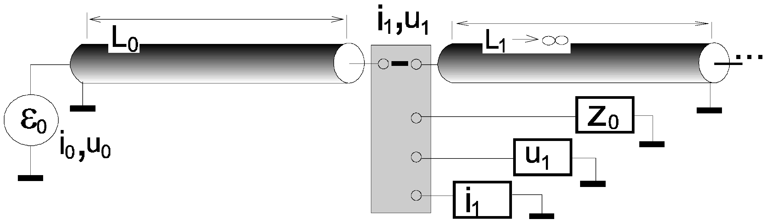
3. The Control of Normal Velocities (Displacements) of the Body’s Surface

Here we consider the problem of quick synthesis of a desired distribution of normal oscillatory velocities (displacements) on the outside surface of an active coating during the time, much smaller, than the characteristic temporal scale of the distribution to be formed. In the absence of incident waves the desired DNOD is zero, and in such a case the active coating solves the radiation suppression problem. In the presence of incident waves the active coating (in addition to suppression of radiation) can (see below) suppress the scattering field of the protected body. In the presence of incident waves the active coating suppresses scattered waves jointly with radiation. This is due to the formation on the external surface of the coating of the normal oscillatory velocities distribution, matched for the incident wave, on the base of signals of some group of microphones (bearing group, see Section 6.2.). The active coating is placed immediately on the surface of the protected body. Below we point to several important characteristics and assumptions in the statement of this problem.

Figure 4. Matching of distribution of normal oscillatory velocities (DNOV) to obtain a "transparent" body (λ - wavelength).

Figure 4. Matching of distribution of normal oscillatory velocities (DNOV) to obtain a "transparent" body (λ - wavelength).

1* Let’s assume, that in the absence of physical scattering surface S_V [outside surface of active coating, which protects some body with a characteristic linear dimension D_V and minimum curvature radius R_V > 0 (Figure 4)] the particle velocities V_⊗ of a non-viscous fluid have the projection υ_{⊗ =} (◊,V_⊗) on the vector ◊ = ◊(r) (which is normal to the surface S_V and with normalized length |◊| = 1, r ∈ S_V). Now, if we created (by means of the active coating) the DNOV [37]:

$$\mathsf{\upsilon }={\mathsf{\upsilon }}_{\otimes }$$

(2)

We would have suppressed the scattering field completely. By the way, the problem of radiation suppression would be solved together with the problem of scattering suppression: without incident waves the normal oscillatory velocity of external surface S_V of the coating must be zero (when nonzero velocity is possible on the internal surface of active coating). The condition (1) must be satisfied in the finite wide operating range of temporal ω and spatial frequencies:

$$\left|\mathsf{\omega }\right|\in ({\mathsf{\omega }}_{\min },{\mathsf{\omega }}_{\max }), \left|\mathsf{\chi }\right|\in ({\mathsf{\chi }}_{\min },{\mathsf{\chi }}_{\max }),$$

(3)

i.e. for a finite area of characteristic spatial and temporal scales:

$$\mathsf{\lambda }\in ({\mathsf{\lambda }}_{\min },{\mathsf{\lambda }}_{\max }),\mathsf{\tau }\in ({\mathsf{\tau }}_{\min },{\mathsf{\tau }}_{\max }),$$

(4)

where ω_min > 0, χ_min = ω_min/c_w, χ_max = ω_max/c_w, where c_w - sound speed in fluid. Wave dimensions of the protected body with a characteristic space scale D_V can be both

$${\mathsf{\chi }}_{\max }{D}_V>>1\mathrm{and}{\mathsf{\chi }}_{\min }{D}_V<<1.$$

(5)

The minimum frequency ω_min must be sufficiently large: this does not permit the displacement magnitude to overcome the border A_max of the linear characteristics of sensors and actuators [10], i.e.:

$${({\mathsf{\omega }}_{\min }{T}_V)}^{-1}{A}_{\otimes }<A_{\max }<<h,$$

(6)

where A_⊗ - desired normal displacement of outside surface of coating, h - its thickness. At ω_min>0 the relation analogous to (2) will be satisfied for normal displacements too.

2* The formation of the current DNOV value υ_⊗ (r,t) at any moment must be fulfilled by some control actions during the short previous time interval of duration T_V << τ_min, much shorter than the minimum temporal scale τ_min of the wave to be suppressed.

3* The thickness h of the active coating (or distance between surfaces $S_V$ and ${\overline{S}}_V$ (Figure 2b) is much smaller than the length of wave, which must be suppressed, i.e. h<<λ.

4* We assume that the protected body has neutral floatability in the outside liquid. The vibroacoustical characteristics of the protected body depend on the temperature and hydrostatic pressure of the outside liquid. It is clear that the control system we need should not include any acoustical interactions with the body, so we will assume below that very little information about the vibroacoustical characteristics of the protected body is available (i.e. it is practically unknown).

5* Literally following the condition 2*, one can get the principal contradiction: formation of a smooth trajectory (normal temporal displacement of the outside coating boundary S_V) by means very short pieces. It would seem that this condition contradicts the traditional control by slow complex magnitudes of the fields, because its spectral power is concentrated close to the current frequency (or, in other words, when both phases and magnitudes of the fields can be determined separately). We remove this contradiction by using very wide spectrum signals. In other words we will form a sequence of short pulses with a smooth average trajectory (inside the range (3), which we need). Further, we will control the normal displacement u(r,t) of the coating outside boundary S_V (instead the normal velocity υ(r,t)) by short periodical blows of duration τ_c and with period T_V >> τ_c (see the description of the algorithm, formula (15) in Section 5.4. below). The spectral power density of desirable displacement u_⊗(r,t) (being averaged over several periods T_V) is concentrated in the range (3),(4). Fast boundary displacements, induced by blow force pulses within short time intervals t ∈ (nT_V, nT_V+ τ_c), we will alternate with relatively slow displacements during long time intervals t ∈ (nT_V–τ_c, (n+1)T_V),) of "relaxation", i.e. "relaxation-blow-relaxation-blow-…" etc, (n=1,2,…). Outside the frequency range (3) we suppose an arbitrary far-field and near-field of waves of a finite power admissible. As a result of the above mentioned control, the average on period [i.e. inside range (3)] normal oscillatory velocity $\overline{\mathsf{\upsilon }}(\mathbf{r},t)=T_V^{-1}{\displaystyle \underset{t-T_V}{\overset{t}{\int }}\mathsf{\upsilon }(\mathbf{r},\mathsf{\xi })d\mathsf{\xi }}$ must be close to the desirable value${\left|\overline{\mathsf{\upsilon }}(\mathbf{r},t)-{\mathsf{\upsilon }}_{\otimes }(\mathbf{r},t)\right|}_{r\in S_V}\to 0$ (or ${\left|u(\mathbf{r},t)-u_{\otimes }(\mathbf{r},t)\right|}_{r\in S_V}\to 0$, as described before), due to the relation:

$$\overline{\mathsf{\upsilon }}(\mathbf{r},t)\cong \{u(\mathbf{r},t)-u(\mathbf{r},t-T_V)\}/T_V.$$

(7)

4. Prior Information About the Construction of the Protected Body

For the considerations that follow we however must make several simple general assumptions to limit the possible vibroacoustical characteristics of the protected body. Several famous essential works, for example [30], are devoted to an interaction between acoustical waves and mechanical structures. Below we will limit our consideration by the simplest rough models.

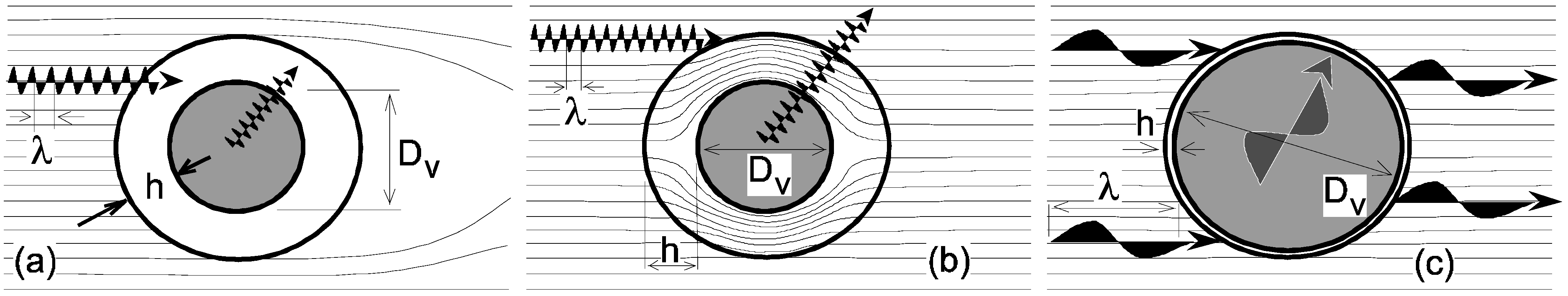
4.1. The Construction of the Protected Body

We assume that the structure of the protected body near its surface represents a closed elastic shell (locally this shell may be analogously the elastic uniform plate) of thickness h with internal surface S., covered outside by polymer layer of thickness h_r (Figure 5).

Figure 5. The assumed structure of protected body with internal discrete connections in the form of mechanical passive chains with impedances Z₁, Z₂, Z₃,…

Figure 5. The assumed structure of protected body with internal discrete connections in the form of mechanical passive chains with impedances Z₁, Z₂, Z₃,…

This layer is a dissipative absorber of the waves with frequencies ≥ π/T_V. The outside surface of the dissipative layer represents the outside surface of the protected body. Many different points within the shell can be connected by various dynamical chains. Possible characteristics of these chains are limited by the following: (a) assumption about low ringingness of the shell (with chains) in liquid; (b) assumption about the spatial and temporal smoothness of the vibration fields of the protected body, Thus, the protected body presents a closed smooth elastic shell, embraced inside by discrete passive dynamic connections (chains), and covered outside by a polymer layer, which is dissipatively opaque for high frequency waves at ω ≥ π/T_V.

4.1.1. Ringingness of the Protected Body

Let’s assume that a weightless layer (with a surface coating ${\overline{S}}_V$) with arbitrary distribution (independent on external pressure) of the velocity (δ/dt)h(r,t) of change of its thickness L(r,t) (or layer of monopole sources) with Fourier image υ₀(r,ω) is limited in the module i.e. |υ₀(r,ω)|≤q₀. This distribution υ₀(r,ω) of monopole sources induces the corresponding distribution υ₀(r,ω) of normal velocities of the surface${\overline{S}}_V$. After this we call the maximum ringingness Q_LF on low frequencies the maximum ratio |υ₀(r,ω)|≤q₀ which was selected using all possible variations of distribution υ₀(r,ω) in all points r of a surface ${\overline{S}}_V$ and on all frequencies of range (3), and analogously we introduce the high frequency ringingness i.e. Q_LF = q_L/q₀ (where q _L= max|υ(r,ω)| among any υ₀(r,ω), $\mathbf{r}\in {\overline{S}}_V$, ω_min < |ω|< ω_max) and Q_HF = q_H/q₀ (where q _H = max|υ(r,ω)| among any υ₀(r,ω), $\mathbf{r}\in {\overline{S}}_V$, $\left|\mathsf{\omega }\right|\ge 2\mathsf{\pi }/T_V$). Of course we are interested in having the values Q_LF and Q_HF as small as possible.

4.1.2. Smoothness of Vibrational Fields on the Protected Body

This assumption about smoothness is caused by the finite elasticity to bending of a body’s parts (or elastic plate) with Young’s modulus E., Poisson’s modulus σ. and mass’s density ρ.. Shell or elastic plates act as filter for low spatial frequencies and for suppression of high spatial frequencies. Let’s consider the simplest problem about excitation of bending oscillations in an infinite plate (spatial filter) with thickness h., induced by the application of normal pressure P₀ = exp(iωt-i)(χ), where χ -spatial frequency. The ratio η. = A/A₀ we will call the transmission coefficient of plate, where A -amplitude of bending oscillations, which was caused by pressure P₀, and A₀ -amplitude of fluid particle displacements in a sound wave in the fluid with pressure P₀, mass density ρ_w and speed c_w of sound. We assume that plate and fluid give the following ratio η. = A/A₀ <<1 on the spatial frequencies |χ|≥π/L_V, where L_V -characteristic linear scale of the active coating splitting (see Section 5.1 below), on all temporal frequencies ω. If the condition

$$L_V^4{\mathsf{\omega }}_{\max }^2{h}_{•}^{-2}<<{(2\mathsf{\pi })}^4{12}^{-1}{(1-{\mathsf{\sigma }}_{•}^2)}^{-1}{E}_{•}{\mathsf{\rho }}_{•}^{-1}$$

(8)

is satisfied, one can use the simple rough estimate:

$$L_V^4{\mathsf{\omega }}_{\max }^2{h}_{•}^{-2}<<{(2\mathsf{\pi })}^4{12}^{-1}{(1-{\mathsf{\sigma }}_{•}^2)}^{-1}{E}_{•}{\mathsf{\rho }}_{•}^{-1}.$$

(9)

Inserting typical practical parameters, i.e. σ. ≈ 0.3, E. ≈ 2x10¹¹, ρ. ≈ 7x10³, ρ_w ≈ 10³, we obtain instead of (8), (9):

$$L_V^4{\mathsf{\omega }}_{\max }^2{h}_{•}^{-2}<<6.2\times {10}^9 \text{(in SI units)}$$

(10)

and

$${\mathsf{\eta }}_{•}\le {10}^{-11}\times (h_{•}^{-3}{L}_V^5{Q}_{LF}{\mathsf{\omega }}_{\max }^2)<<1,$$

(11)

Note, that the estimate (11) can only be of any practical interest at h.<< L_V.

4.1.3. Constancy of Parameters of the Protected Body

Within the bounds of the temporal interval ${\mathsf{\tau }}_s>>D_V/c_w$ we will assume constant the parameters of the protected body. The solution suggested does not require constancy of parameters for a long time.

4.1.4. Layer of Dissipative Polymer

This polymer layer of thickness h_r and longitudinal impedance Z_r is spaced immediately on the external surface S. of an elastic plate (shell). We will assume that Z_r satisfies the condition |Z_r-Z_c|/|Z_c|<<1 (where Z_c is a longitudinal impedance of the active coating, see below) within the frequency range ω_min ≤ 2π/T_V. We thus assume the surface S_V transparent for the waves of the range above mentioned. Besides this, we assume that on the frequencies ~π/ T_V the distance l_r of dissipative relaxation of waves in e-times satisfies conditions λ_min>>h_r and h_r >> l_r. It is clear that we can combine these conditions only if the condition h_r >> c_rT_V is satisfied, where c_r - speed of sound in the polymer. This polymer layer thus gives a significant reduction of high frequency ringingness Q_HF to the protected body.

5. Active Coating and its Control Algorithm

We place immediately on the external surface of the protected body (i.e. on the high frequency dissipative polymer layer) the active coating of thickness D = 2h_c << λ_min in the form of two piezoelectric layers of thickness h_c (each layer), with identical polarization along the normal to ${\overline{S}}_V$. We assume that the longitudinal impedance Z_c = ρ_cc_c of the piezoelectric material is equal to the impedance Z_w = ρ_wc_w of the outside liquid (i.e. Z_c = Z_w ), where ρ_c-mass density of piezoelectric material and ρ_w-mass density of outside liquid and correspondingly, c_c-speed of longitudinal sound in the piezoelectric material, c_w-speed of sound in the outside liquid. The total thickness of the body and coating cross sectional structure L = h. + h_r + 2h_c (see Figure 6c). For certainty we will assume c_c > c_w.

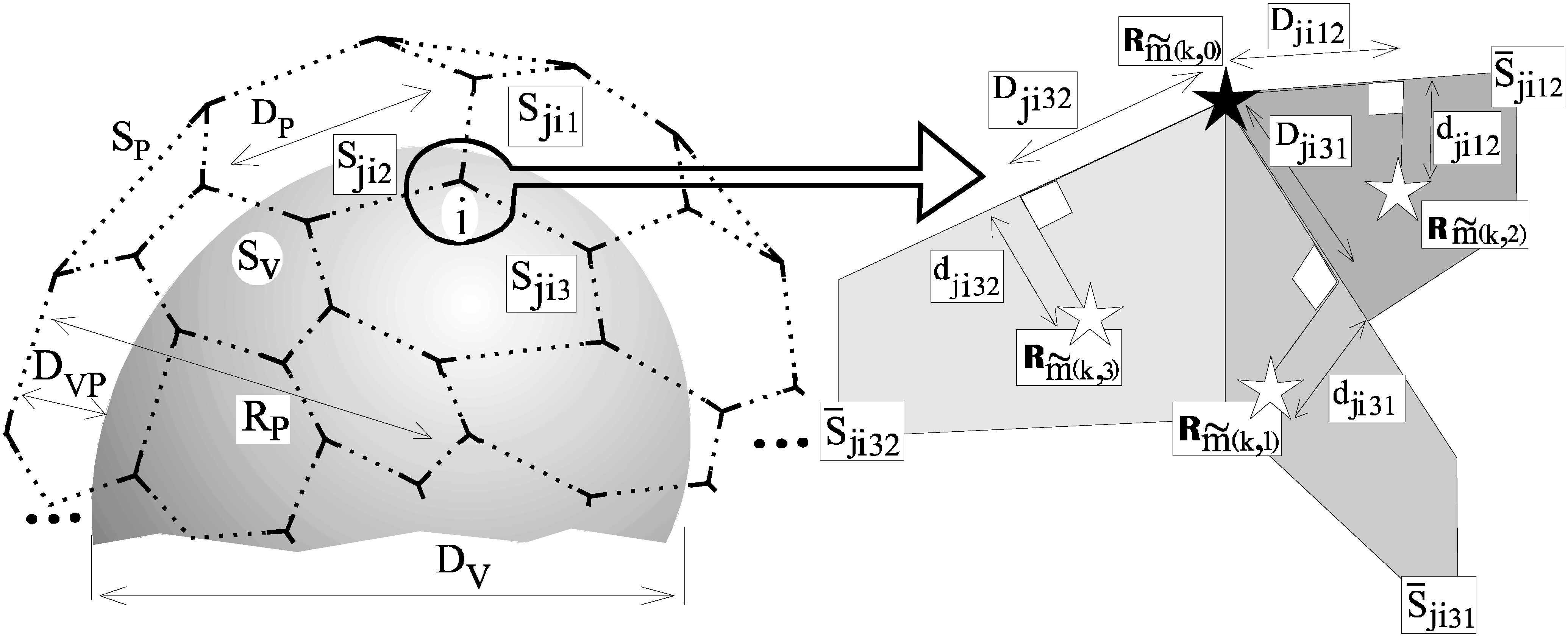
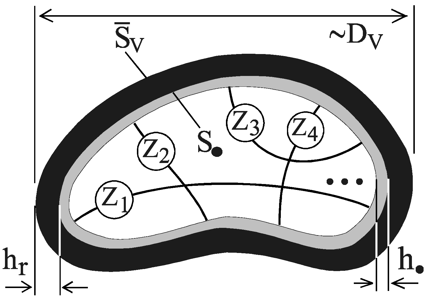
5.1. The Discrete Representation of the Body Protection Surface

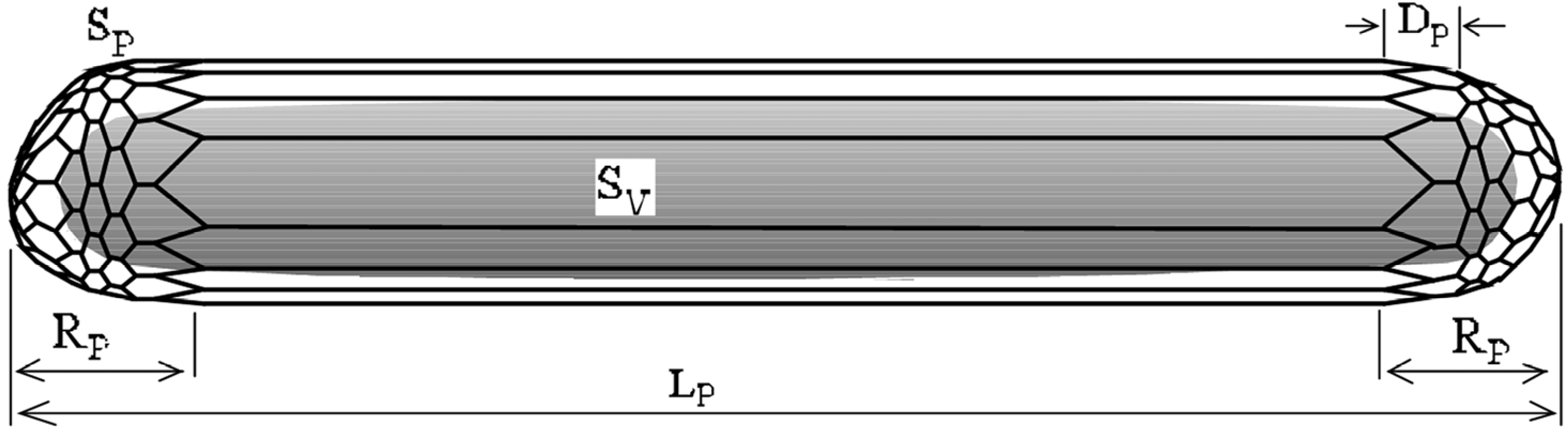
Let’s divide the surface ${\overline{S}}_V$ into a set of N_V >> 1 monopole-like radiating pistons S_k (“equivalent pistons”) (k = 1,2,…,N_V,,${\displaystyle \underset{k\ne m}{\cap }{S}_k{S}_m=0}$, ${\displaystyle \underset{\forall k}{\cup }{S}_k={\overline{S}}_V}$, Figure 6a, Figure 11b). Each equivalent piston S_k is represented by the prominent polygon with square σ_k [37] and characteristic linear scale ~L_V, satisfying the following conditions L_V < λ_min/2 and L_V >> h_r + 2h_c. Within each equivalent piston S_k (i.e. for r ∈ S_k) we suppose DNOV υ(r,t) = υ_k(t) is constant and also another constant DNOV within another pistons. Normal velocity of external surface of each k-th piston (spatial constant on S_k) is equal to: ${\mathsf{\upsilon }}_k(t)={({\mathsf{\sigma }}_k)}^{-1}{\displaystyle \underset{S_k}{\iint }\mathsf{\upsilon }(\mathbf{r},t)dS}$, where υ(r,t) is the initial velocity, forming the smooth DNOV on ${\overline{S}}_V$ (i.e. before the beginning of action of control system). At the distance $r>L_V^2/{\mathsf{\lambda }}_{\min }$ from ${\overline{S}}_V$ the sound, produced by DNOV υ(r,t), practically does not differ from the sound produced by corresponding system of N_V "equivalent pistons".

5.2. Active Coating

Now we place "active pistons" ${\overline{S}}_k$, identically covering the "equivalent pistons" S_k, described above. Each ${\overline{S}}_k$ is of the same shape and square like S_k. Each active piston ${\overline{S}}_k$ is characterized by its “mass center”:

$${\mathsf{\rho }}_k={({\mathsf{\sigma }}_k)}^{-1}{\displaystyle \underset{{\overline{S}}_k}{\iint }\mathbf{r}dS}$$

(12)

where σ_k -square of the equivalent piston S_k (or of active piston ${\overline{S}}_k$, Figure 6-a,b). The characteristic linear dimension ~L_V of each piston is much smaller than the value 2π/w_Q (i.e. L_V <<2π/ω_Q), where the frequency ω_Q will be determined in Section 6.3. below. Each active piston ${\overline{S}}_k$ represents a so-called "Huygens’s piston". Such a piston produces waves of radiation only on one side (external). All together N_V>>1 Huygens’ pistons form the active coating of the protected body. This coating is placed between the closed surfaces ${\overline{S}}_V$ (internal) and surface S_V (external). The problem of control of radiation and scattering means the formation of the desired (DNOV) distribution of normal oscillatory velocities (displacements) on the surface S_V.

Figure 6. Tangential (a, b) and cross-section (c) structure of the protected body and active coating.

Figure 6. Tangential (a, b) and cross-section (c) structure of the protected body and active coating.

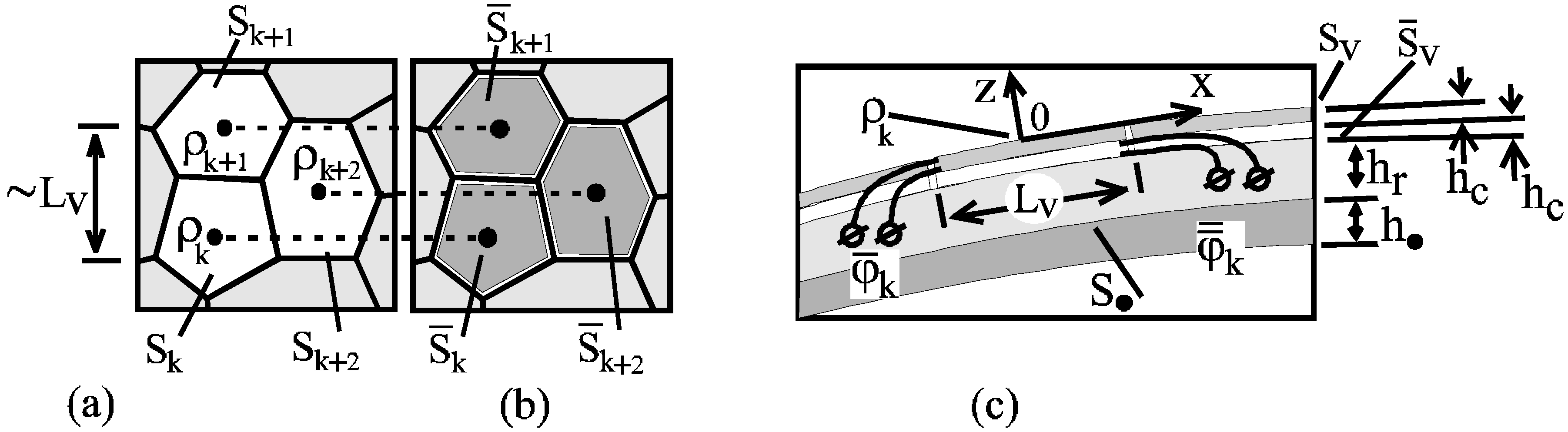
5.3. The Cross-Section Structure of the Protected Body

Each Huygens’ piston (or active piston) ${\overline{S}}_k$ represents two layers (two piezoelectric layers, which were polarized identically along the axis "z", Figure 6c) in cross-section. In top view Huygens’ piston presents a planar convex polygon. In other words the active coating is divided into a lot (N_V>>1) of Huygens’ pistons (Figure 6b) analogous to the pistons S_k, called above radiating pistons. Equivalent pistons S_k and active pistons ${\overline{S}}_k$ (Huygens’s) have the same "mass’s center" ρ_k, the same square σ_k and the same characteristic linear spatial scale ~L_V. Surfaces of each piezoelectric layer are covered by thin metal weightless films and equipped by electric contacts (Figure 6c). Between contacts of each k-th Huygens’ piston the differences ${\overline{\mathsf{\phi }}}_k(t)$ and ${\overline{\overline{\mathsf{\phi }}}}_k(t)$ of the electric potentials are supported by active control system.

5.4. The Control Algorithm for the Synthesis of DNOV

The electric voltages, which are applied to each layer of the k-th Huygens’ piston, have a view:

$${\overline{\mathsf{\phi }}}_k(t)=\underset{n=0}{\overset{[t/T_V]}{\Sigma }}{B}_{n,k}{\overline{\mathsf{\phi }}}_B(t-n{T}_V),{\overline{\overline{\mathsf{\phi }}}}_k(t)=\underset{n=0}{\overset{[t/T_V]}{\Sigma }}{B}_{n,k}{\overline{\overline{\mathsf{\phi }}}}_B(t-n{T}_V),$$

(13)

and can be presented by the temporal sequence of pulses (Figure 7a,b):

$${\overline{\mathsf{\phi }}}_B(t)=\{I(t)-I(t-{\mathsf{\tau }}_c)\}{\mathsf{\phi }}_0 \text{and} {\overline{\overline{\mathsf{\phi }}}}_B(t)=-{\overline{\mathsf{\phi }}}_B(t-{\mathsf{\tau }}_V)$$

(14)

with period T_V and duration 3τ_V (or 3T_V/2), where we introduced the time τ_V during which wave overcomes the distance between the boundaries of one piezoelectric layer. There we supposed I(ξ)=1 at ξ > 0, I(ξ)=0 at ξ ≤ 0, ϕ₀=const . The magnitude B_n,k of these pulses is determined by the formula:

$$B_{n,k}={({\mathsf{\psi }}_0{T}_V/2)}^{-1}{\displaystyle \underset{n{T}_V-T}{\overset{n{T}_V}{\int }}\overline{F}(Y_k-Y_{\otimes k})dt}$$

(15)

where$Y_k(t)={\mathsf{\sigma }}_k^{-1}{\displaystyle \underset{S_k}{\iint }u(\mathbf{r},t)d{S}_k}$, $Y_{\otimes k}(t)={\mathsf{\sigma }}_k^{-1}{\displaystyle \underset{S_k}{\iint }{u}_{\otimes }(\mathbf{r},t)d{S}_k}$, T- temporal interval of averaging, ψ₀ = const. - amplitude of basic bipolar pulse of displacement, [ξ] means the whole part of number ξ, u_⊗ (r,t) and u(r,t) - perfect and real (measured) normal displacements of surface S_V. The operator $\overline{F}[q]={\displaystyle \underset{0}{\overset{t}{\int }}F(t-\mathsf{\xi })q(x,y,\mathsf{\xi })d\mathsf{\xi }}$ represents a linear filter with frequency transmission coefficient $\tilde{F}(\mathsf{\omega })={\displaystyle \underset{0}{\overset{t}{\int }}F(t)\exp (i\mathsf{\omega }t)dt}$. The module of the last near zero frequency has the form $\left|\tilde{F}(\mathsf{\omega })\right|~{\left|\mathsf{\omega }\right|}^{2\mathsf{\epsilon }}$ (ε -whole positive number). On the frequencies of range (3) (and up to the frequencies $~T_V^{-1}$) its module is $\left|\tilde{F}(\mathsf{\omega })\right|=1$. The relation between the mechanical ψ₀ and electric ϕ₀ magnitudes is determined by the formula ψ₀/ϕ₀ = (τ_c/h_c)(ε₀ε_cη_c/E_c)½, where ε₀-dielectric constant of vacuum, E_c -Young’s modulus of piezoelectric material, η_c-coefficient of electro-mechanical connection in piezoelectric (η_c ~ 0.2 ÷ 0.8). In analog representation the filter $\overline{F}$ can be described as electric differential RC -circuit with time scale τ_RC>>τ_max. In accordance with (16) the amplitude B_n,k of electric pulses ${\overline{\mathsf{\phi }}}_B(t-n{T}_V)$ and ${\overline{\overline{\mathsf{\phi }}}}_B(t-n{T}_V)$, acting correspondingly in the temporal intervals:

$$n{T}_V\le t<n{T}_V+{\mathsf{\tau }}_c\text{ and }n{T}_V+{\mathsf{\tau }}_V\le t<n{T}_V+{\mathsf{\tau }}_V+{\mathsf{\tau }}_c (n=1,2,\dots ).$$

(16)

(u-u_⊗) is the error signal, which one had averaged spatially (instantly in time) along the surface of piston ${\overline{S}}_k$ and also averaged in time [15] on the previous temporal interval nT_V – T ≤ t < nT_V, where T=m(3τ_V+τ_c) (m=1,2,…). Time interval of averaging satisfies the condition ${\displaystyle \underset{0}{\overset{T}{\int }}{\Psi }_B(t)dt}=0$.

Voltages ${\overline{\mathsf{\phi }}}_k(t)$, ${\overline{\overline{\mathsf{\phi }}}}_k(t)$ form the field:

$$\mathsf{\psi }(\mathbf{r},t)=\underset{n=0}{\overset{[t/T_V]}{\Sigma }}{B}_{n,k}{\mathsf{\psi }}_B(\mathbf{r},{\mathsf{\rho }}_k;t-n{T}_V)$$

(17)

of normal displacements of the surface S_V. The function $B_{n,k}{\Psi }_B(\mathbf{r},{\mathsf{\rho }}_k;t-n{T}_V)$ represents the normal displacement in the point $\overrightarrow{r}\in {\overline{S}}_k$ (Figure 7c), created by pulses $B_{n,k}{\overline{\mathsf{\phi }}}_B(t-n{T}_V)$, $B_{n,k}{\overline{\overline{\mathsf{\phi }}}}_B(t-n{T}_V)$ of electric voltage of duration τ_c<<τ_V, respectively, on the external and internal layers of the active piston ${\overline{S}}_k$ (with center in the point ρ_k) at the moments t = nT_V and t=nT _V + τ_V .

It was shown [15], that in a one-dimensional problem (at L_V →∞) such a double layer of piezoelectric material (or piston) with the above mentioned magnitude-temporal relation (Figure 7с) between inducing electric pulses (Figure 7a,b) creates a Huygens’ source (or Huygens’ piston).

Figure 7. The shape of pulse of electric voltage${\overline{\phi }}_B(t)$, which is applied to external layer of $z\in (-h_c,0)$ active piston (a); shape of pulses of electric voltage ${\overline{\overline{\mathsf{\phi }}}}_B(t)$, which is applied to internal layer $z\in (-2h_c,-h_c)$ of active piston (b); shape of "basic pulses" ${\Psi }_B(\mathbf{r},{\mathsf{\rho }}_k;t)$ of normal displacement of outside surface $S_k$ of piston, which was created by electric pulses above mentioned on a distance |r – ρ_k| <c_wt,L_V)) from the border of piston ${\overline{S}}_k$ (or in the locally one-dimensional problem) (c).

Figure 7. The shape of pulse of electric voltage${\overline{\phi }}_B(t)$, which is applied to external layer of $z\in (-h_c,0)$ active piston (a); shape of pulses of electric voltage ${\overline{\overline{\mathsf{\phi }}}}_B(t)$, which is applied to internal layer $z\in (-2h_c,-h_c)$ of active piston (b); shape of "basic pulses" ${\Psi }_B(\mathbf{r},{\mathsf{\rho }}_k;t)$ of normal displacement of outside surface $S_k$ of piston, which was created by electric pulses above mentioned on a distance |r – ρ_k| <c_wt,L_V)) from the border of piston ${\overline{S}}_k$ (or in the locally one-dimensional problem) (c).

This double layer provides a bipolar pulse of media particles displacement of duration T_B = 3τ_V + τ_c. These pulses are moving through space (like wavelets [36], Figure 8) with speed c_w. A wavelet (we will also call it a "basic pulse") is only radiated forwards (outside the surface S_V) and must always contain an interval of zero magnitude and of duration τ_V, between two pulses of mutually opposite polarity and same duration τ_V. At the back (z <-2h_c) the pulses, induced by both piezoelectric layers, move and add to mutually opposite phases giving a zero sum in the backspace (inside${\overline{S}}_V$, Figure 8).

Figure 8. “Huygens’ piston” of finite dimensions L_V + L_V in the homogeneous free compressible space and the instant spatial distributions of media particles displacements are represented by a running "basic pulses" Ψ_B(z,t) (at |r – ρ_k| < c_wt,L_V)) (an external side of an active piston), induced by piezoelectric layers (and zero pulses at internal side of active piston). Darker pulses (waves) are produced by the electric voltage ${\overline{\mathsf{\phi }}}_B(t)$ layer of active piston. Less dark pulses (waves) are induced by the electric voltage ${\overline{\overline{\mathsf{\phi }}}}_B(t)$.

Figure 8. “Huygens’ piston” of finite dimensions L_V + L_V in the homogeneous free compressible space and the instant spatial distributions of media particles displacements are represented by a running "basic pulses" Ψ_B(z,t) (at |r – ρ_k| < c_wt,L_V)) (an external side of an active piston), induced by piezoelectric layers (and zero pulses at internal side of active piston). Darker pulses (waves) are produced by the electric voltage ${\overline{\mathsf{\phi }}}_B(t)$ layer of active piston. Less dark pulses (waves) are induced by the electric voltage ${\overline{\overline{\mathsf{\phi }}}}_B(t)$.

The main difference between of the suggested approach and traditional approaches is concerned with the following. Usually the desired trajectory (temporal) of the normal displacement of S_V can be achieved by the temporal sequence of pulses without their intersection and with nonzero mean value of each pulse (for instance - delta pulse). In the algorithm of the synthesis of desired trajectory, described below, we use bipolar pulses mutually intersecting with: zero mean value, duration T_B = 3τ_V + τ_c (where τ_c << τ_V), temporal period T_V = 2<< τ_V of sequence. Each main pulse consists of three consequent identical intervals << τ_V. The first (left part) interval of the next basic pulse is covered by the third (right part) interval of the previous basic pulse. The absence of the source (one-dimensional [36]) and wave field in back-space means that we can generate forward radiation waves without any mechanical support of both piezoelectric layers, due to the special construction of the Huygens’ source. Besides one-side radiation this Huygens’ source is an acoustically transparent source. The wave, which was radiated by a Huygens’ source, does not depend on impedance in back-space and can be simply added to any wave passing without any interaction with the source. In [36] we can see the same effect of the one side radiation without mechanical support for the monochromatic excitation (on some frequency ω) of two piezoelectric layers (with the phase difference Δϕ = ωh_c/c_c of excitation). A very small phase difference (necessary for one side radiation) is defined by stationary device tuning. This phase difference does not depend of acoustical field, measured by sensors. So the measurement errors ~Δψ (which determines phase and magnitude of one-side radiation) of the acoustical field is included coherently (with mutually opposite signs) into both voltages, exciting both piezoelectric layers, and cannot cause the growth of the unbalance of waves in ~Δψ/Δϕ >>1 times. Note that in the absence of incident waves the algorithm (15) can be used for radiation suppression, when $Y_{\otimes k}(t)\equiv 0$.

5.5. Some Notes about the Stability of the Synthesis of DNOV (DNOD)

The interaction between elements of an active damping system always presents possible channels of instability, so it follows that the absence of interaction would also mean the absence of instability. Now we will consider very briefly the main types of interactions in the system of DNOV synthesis. We will consider below the two planes z = 0 (analog of surface S_V) and z = -2h_c (analog of surface ${\overline{S}}_V$) filled with Huygens’ pistons (two layers of piezoelectric material). This pair of planes is in contact outside with a half-infinite compressible homogeneous space. In addition we assume that the compressibility and speed of propagation of acoustical waves are same in the piezoelectric material and the outside compressible media. This becomes possible due to the use of piezoelectric materials, containing polymers [33,35]. Now we can achieve the continuum spectrum of electromechanical characteristics of such piezocomposite materials with ceramics and polymers [33]. Below we try to explain the smallness of the interaction effects when using the algorithm (15).

5.5.1. Interaction Between Adjacent Pistons

The control algorithm (15) is a three-dimensional one (discrete spatially and temporally) and presents the generalization of the one-dimensional solution [36] without diffraction waves. In general the dynamics of the surface S_V can be described as a sequence of: (a) fast (during a time τ_c << T_V one-side blows, spatially uniformly distributed along a Huygens’ piston, when the error (Yk - Y_⊗k) ≠ 0 of the k-th piston jumps to zero (during the time τ_c), forming the "imprint"; (b) slow linear growth of |Yk - Y_⊗k| in a time not quicker, where is a life-time of "imprint" (time of its diffraction relaxation), A_⊗ - characteristic magnitude of the desired displacement u_⊗(t) of the surface S_V, Q_LF -body’s ringingness at low frequencies (Section 4.1.1 and Section 4.1.2). The condition ${\overline{T}}_V=L_V/c_w>>T_V$ is the principal one for our active system, due to which we can neglect the interaction between adjacent pistons and the value of the corresponding positive feedback ${\mathsf{\gamma }}_1={(T_V/{\overline{T}}_V)}^2<<1$.

5.5.2. Synthesis of One-Dimensional DNOD in a Three-Dimensional Case

This case is thoroughly described in [36], and we present here only result of the spatially uniform (along the plane) synthesis shown in Figure 9a,b. There the desired continuous trajectory u_⊗(t) we approximate by the consequence u_⊗(t) of “rectangular” displacement pulses of duration τ_V with period T_V = 2τ_V (Figure 9b). So to obtain the desired DNOV, we need to average this over the temporal period T_V. Effects of diffraction are not considered, because this case is physically equivalent to the spatially one-dimensional case (absence of any border waves).

Figure 9. Infinite plane array, formed from a lot of sources of Huygens’ (strip-like) pistons. One-dimensional (a) synthesis (in accordance with algorithm (15)) of desired spatially uniform DNOD u_⊗(t) (b) by sequence p(t) pressure pulses (of duration τ_c and temporal period τ_V) of uniformly distributed pressure blows, applied to boundary z = 0. Step-like excitation of plane array (c): transient deformations of the boundary z = 0, caused by the first two pulses of pressure (white arrow), applied to the half-plane x ≥ 0 (d).

Figure 9. Infinite plane array, formed from a lot of sources of Huygens’ (strip-like) pistons. One-dimensional (a) synthesis (in accordance with algorithm (15)) of desired spatially uniform DNOD u_⊗(t) (b) by sequence p(t) pressure pulses (of duration τ_c and temporal period τ_V) of uniformly distributed pressure blows, applied to boundary z = 0. Step-like excitation of plane array (c): transient deformations of the boundary z = 0, caused by the first two pulses of pressure (white arrow), applied to the half-plane x ≥ 0 (d).

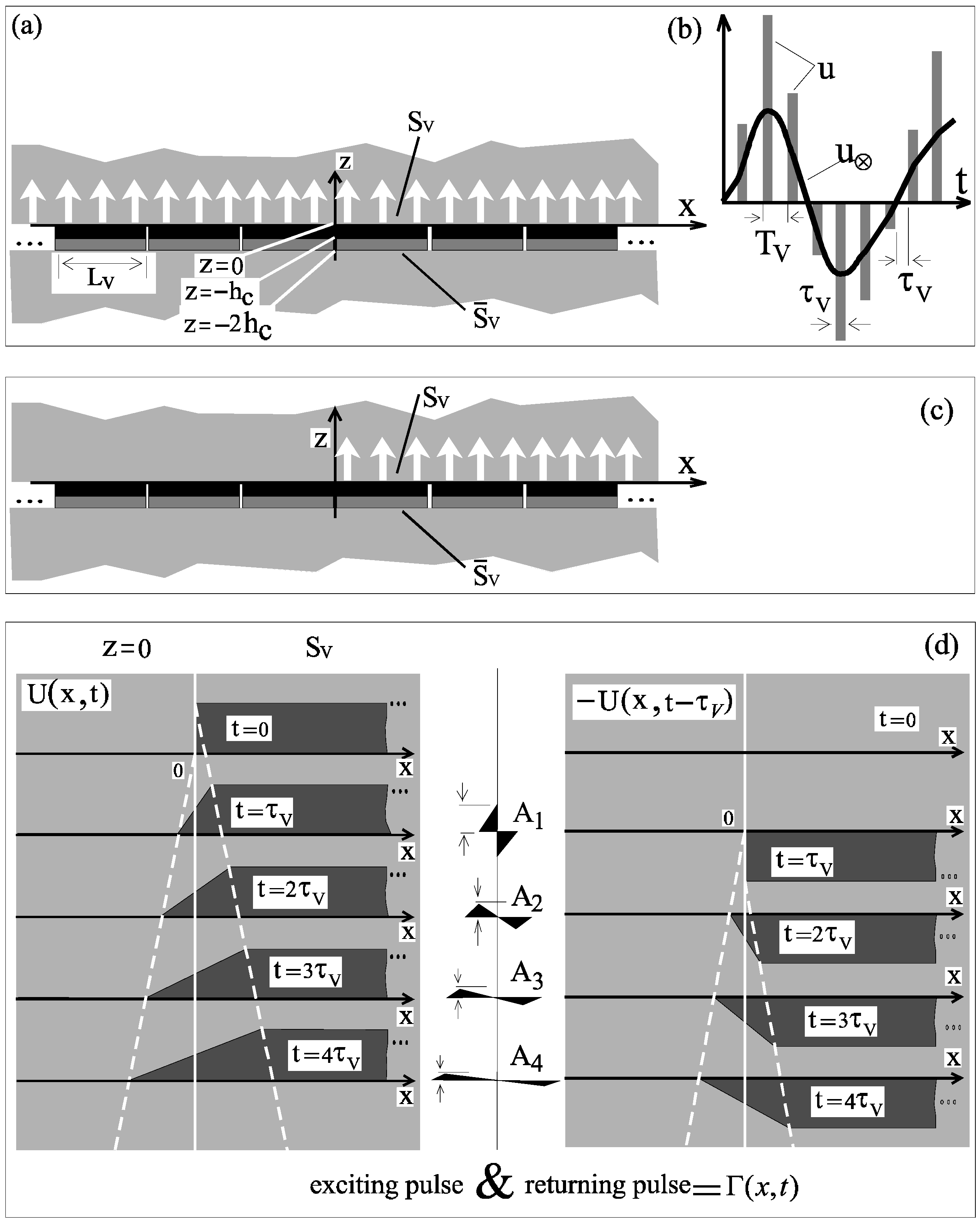
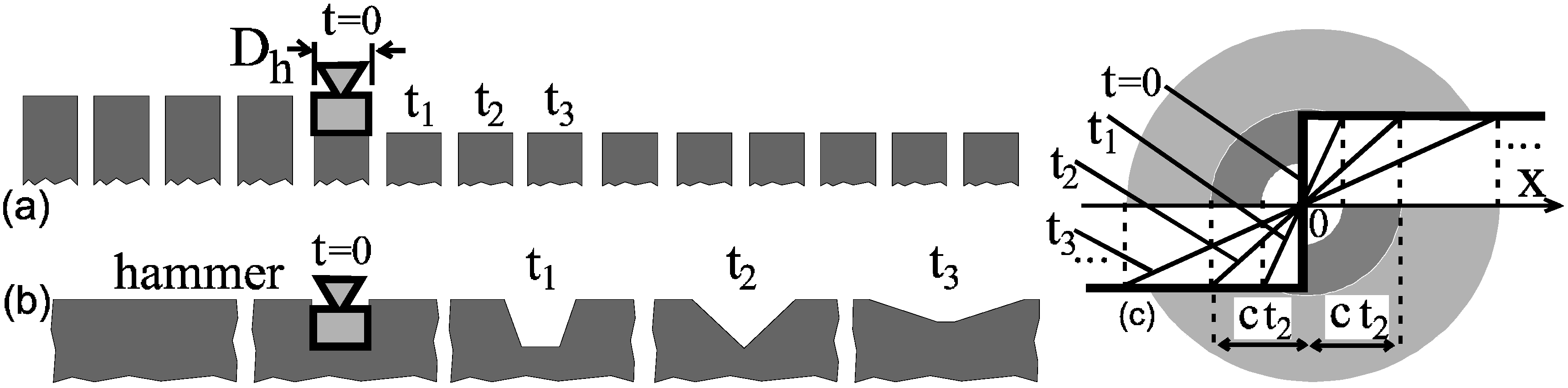
5.5.3. Formation of Step-Like DNOD

Now we consider the case of spatially uniform blow on a half-infinite plane part of the border (Figure 9c). In the center of this figure we see instant photos of the superposition Γ(x,t) of left U(x,t) and right U(x,t- τ_V) waves at the moments t = mτ_V (m = 0,1,2,…). Here we assume that U(x,0) = A I(x), if t = 0, where I(x)= 0, if x<0 and I(x) = 1, if x≥0, A -magnitude. First a step-like pulse of pressure (without any reaction to the back) excites the array and creates during τ_c the step-like DNOD U(x,τ_c). In a time t > τ_V the returning pulse of force appears and causes DNOD with shape -U(x,t-τ_V). It is shown that function Γ(x,t) = U(x,τ_c) - U(x,t-τ_V) is spatially bipolar (spatial averaging gives zero) and its magnitudes A₁ > A₂ > A₃, … (Figure 9d) are characterized by a quick monotone decrease, which characterizes the intensity of back radiation of the plane array of Huygens’ pistons at two pressure blows (of mutually opposite sign, of step-like shape, and with temporal shift) together.

5.5.4. Formation of Strip-Like Piston DNOD

We get a strip-like DNOD Π(x,t), in the form Π(x,t) = Γ(x,t) - Γ(x - L_V,t), i.e. strip of width L_V. This combination cannot lead to the growth of border waves described in the previous Section 5.5.3. For instance at t = T_V we have |Π(x, T_V)| <c_wτ_V/L_V << 1 and so on at x,t → ∞. So the transient waves (Figure 9d, center) of normal displacement are bipolar and have small spatial scale (elastic plates in the body’s shell almost do not respond to these waves, see Section 4.1.2.) and small time scale (damped by high frequency dissipation in the polymer layer on the shell) or have very small magnitude. We considered the several first pulses of the piston array and have obtained a tendency of evolution of transient processes. Unlike Π(x, t), a real strip-like DNOD, created by an array of strip-like pistons [controlled by algorithm (15)], represents an “arbitrary” DNOD U(x, t), constrained by the following conditions:$L_V^{-1}{\displaystyle \underset{(n-1)L_V}{\overset{n{L}_V}{\int }}U(x,t)=0}$, if $n\notin 0$ and $L_V^{-1}{\displaystyle \underset{(n-1)L_V}{\overset{n{L}_V}{\int }}U(x,t)=A}$, if n = 0. We note again, as was described in Section 5.5, that the control blows create the desired "imprints" during a very short time τ_c, and this "imprint" relaxes during long time L_V/c_w. Besides this, the radiation of the (strip-like) active array to the back (towards the protected body) has a spatial spectrum, which is concentrated near the frequencies |χ| ≥ π/L_V [due to the periodical zero intervals in the temporal representation of the field of pressure blows (Figure 9b)]. So the back radiation of the active coating does not act on the surface $S_{•}$ (see Section 4.1.). Besides this any the wave with spatial frequency |χ| ≥ π/L_V relaxes due to the high frequency dissipation in the polymer layer between surfaces $S_{•}$ and ${\overline{S}}_V$. Now we can quickly construct an arbitrary desired DNOV on S_V as a superposition of these pressure blows, and we can neglect the oscillation of the shell, caused by the active coating.

5.5.5. About Ringingness of a Body

Instability can be caused by unlimited growth of the previous blow contributions of all pistons. Such a scenario can be possible in the following cases: (a) if Q_LF >> 1, when an active coating is placed on the surface of resonator mirrors (for instance, as an analog of the protected body), and the desired DNOV would "intersect" with some own resonator’s mode of infinite ringingness; (b) when the high frequency ringingness is too large (see Section 4.1.1., Section 4.1.2.), i.e. Q_HF >> 1. Thus, the body’s ringingness Q_LF in a passive system can be interpreted as a natural (passive) positive feedback with coefficient ${\mathsf{\gamma }}_{+}\approx Q_{LF}/(1+Q_{LF})<1$. In a passive system always ${\mathsf{\gamma }}_{+}<1$, but in active systems the feedback coefficient ${\mathsf{\gamma }}_{+}>1$ is possible, and may cause instability.

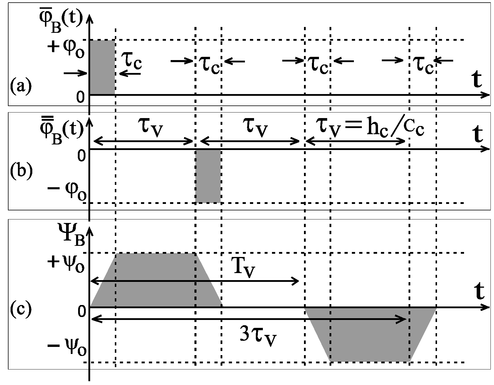
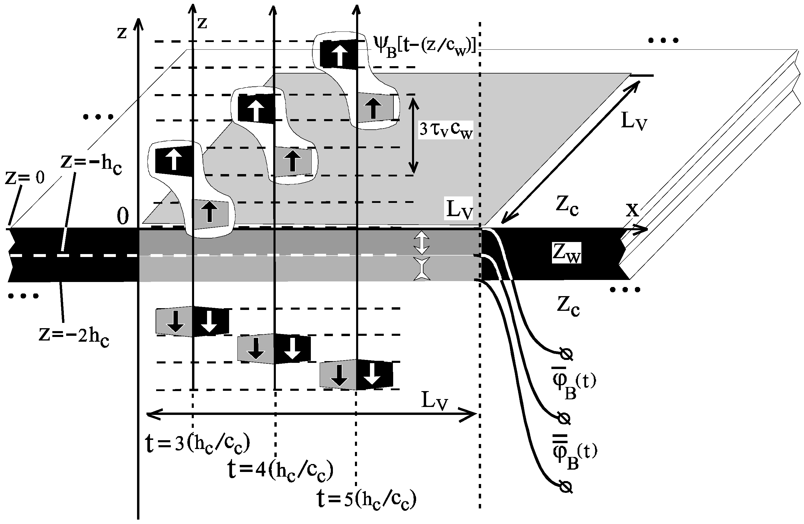
5.5.6. Hierarchy of Scales in the Active Coating

Besides the algorithm (15), to ensure the effective formation of the desired DNOV (DNOD) on S_V we need to use the following hierarchy of system parameters:

$$A_{\otimes }/c_w<<{\mathsf{\tau }}_c<<T_V<<L_V/c_w<<h_r/c_r<<R_V/c_w,{\mathsf{\tau }}_{\min },$$

(18)

where τc -duration of electric voltage pulse on piezoelectric layers of the Huygens’ piston (or duration of a blow on S_V), T_V-temporal period of control actions (blows), h_r-thickness of polymer layer of high frequency dissipation, c_r-speed of propagation of longitudinal sound in polymer, L_V-characteristic tangential linear dimension of a piston, c_w-sound speed in the outside compressible media (liquid), τ_min -minimum period of the waves damped, R_V-minimum curvature radius of the surface S_V, A_⊗-characteristic magnitude of a desired normal displacement $u(\mathbf{r},t)$.

5.6. The Measuring Section of the Active Control Damping System

The control system tries to minimize the difference between three, generally speaking, physically non-identical values: (1) desired [in accordance with control algorithm (15)] normal displacement of surface S_V; (2) real normal displacement of surface S_V; (3) measured normal displacement of surface S_V. In this section we will formulate the way to measure the value Y_k(t) [see (15)]. Let’s direct the axis "z" to the external media (Figure 6c) along the normal of the k-th (k=1,2,3,…,N_V) active piston ${\overline{S}}_k$ with point z = 0 (which is identical with the piston’s center ρ_k) and with square σ_k. Now we cover the boundaries z = 0 (surface S_V), z = –h_c, z = –2h_c (surface ${\overline{S}}_V$), z = –2h_c – h_r (surface $S_{•}$) by thin weightless metal film between the outside media, the piezoelectric layers –h_c ≤ z ≤ 0 and –2h_c ≤ z ≤ –h_c [with relaxed thickness h_c = h_c(r) and $h_c={\overline{h}}_c(\mathbf{r})$ respectively], and polymer layer –2h_c –h_r ≤ z ≤ –2h_c [with relaxed thickness h_r = h_r(r)], and outside surface $S_{•}$ of the shell. So we obtain, respectively, three plane electric capacities:

$${\overline{C}}_k(t)={\mathsf{\epsilon }}_0{\mathsf{\epsilon }}_c{\mathsf{\sigma }}_k{\displaystyle \underset{S_k}{\iint }[h_c(\mathbf{r})}+\overline{h}(\mathbf{r},t){]}^{-1}d{S}_k={\overline{J}}_k(t)/[d{\overline{\overline{\mathsf{\phi }}}}_k(t)/dt]$$

$${\overline{\overline{C}}}_k(t)={\mathsf{\epsilon }}_0{\mathsf{\epsilon }}_c{\mathsf{\sigma }}_k{\displaystyle \underset{S_k}{\iint }[h_c(\mathbf{r})}+\overline{\overline{h}}(\mathbf{r},t){]}^{-1}d{S}_k={\overline{\overline{J}}}_k(t)/[d{\overline{\overline{\mathsf{\phi }}}}_k(t)/dt],$$

$${\overline{\overline{\overline{C}}}}_k(t)={\mathsf{\epsilon }}_0{\mathsf{\epsilon }}_r{\mathsf{\sigma }}_k{\displaystyle \underset{S_k}{\iint }[h_c(\mathbf{r})}+\overline{\overline{\overline{h}}}(\mathbf{r},t){]}^{-1}d{S}_k={\overline{\overline{\overline{J}}}}_k(t)/[d{\overline{\overline{\overline{\mathsf{\phi }}}}}_k(t)/dt],$$

where ε_c, ε_r, -relative dielectric constants of piezoelectric and polymer, respectively; $\overline{h}(\mathbf{r},t)$,$\overline{\overline{h}}(\mathbf{r},t)$,$\overline{\overline{\overline{h}}}(\mathbf{r},t)$ are the instant fields of thickness changes of layers –h_c ≤ z ≤ 0, –2h_c ≤ z ≤ –h_c, –2h_c –h_r ≤ z ≤ –2h_c of piezoelectric material and polymer, respectively;${\overline{\mathsf{\phi }}}_k(t)$,${\overline{\overline{\mathsf{\phi }}}}_k(t)$,${\overline{\overline{\overline{\mathsf{\phi }}}}}_k(t)$ the measured voltages on the corresponding capacities;${\overline{J}}_k(t)$,${\overline{\overline{J}}}_k(t)$, ${\overline{\overline{\overline{J}}}}_k(t)$ the measured charging currents. It is easy to see that at $h_c(\mathbf{r})>>\overline{h}(\mathbf{r},t)$, $h_c(\mathbf{r})>>\overline{\overline{h}}(\mathbf{r},t)$, the spatially averaged value (along S_k) $H_k(t)={\mathsf{\sigma }}_k^{-1}{\displaystyle \underset{S_k}{\iint }[\overline{h}(\mathbf{r},t)+\overline{\overline{h}}(\mathbf{r},t)}+\overline{\overline{\overline{h}}}(\mathbf{r},t)]d{S}_k$ of change of total thickness of two piezoelectric layers and one polymer layer is expressed via measured capacities ${\overline{C}}_k(t)$,${\overline{\overline{C}}}_k(t)$,${\overline{\overline{\overline{C}}}}_k(t)$ as the following: $H_k(t)=h_c\left[\frac{{\overline{C}}_k(t)}{{\overline{C}}_k^o}-1\right]+h_c\left[\frac{{\overline{\overline{C}}}_k(t)}{{\overline{\overline{C}}}_k^o}-1\right]+h_r\left[\frac{{\overline{\overline{\overline{C}}}}_k(t)}{{\overline{\overline{\overline{C}}}}_k^o}-1\right]$, where ${\overline{C}}_k^0$, ${\overline{\overline{C}}}_k^0$, ${\overline{\overline{\overline{C}}}}_k^0$ - relaxed values of capacities ${\overline{C}}_k(t)$, ${\overline{\overline{C}}}_k(t)$, ${\overline{\overline{\overline{C}}}}_k(t)$. Knowing the value $H_k(t)$ and the normal displacement U_k(t) of the boundary z = –2h_c – h_r, averaged along the area S_k, we would obtain the value $Y_k(t)=H_k(t)+U_k(t)$ [used in algorithm (15)]. However, the statement of the problem in this work (see Introduction) excludes the usage not only of mechanical support(s) for active pistons (dynamical vibrostat), but also excludes the usage of any inertial coordinate system (cinematic vibrostat), relatively with which we would like to measure normal displacements of controlled surface. We can measure the displacement G(ρ_k,t) of boundary z = –2h_c–h_r in the center ρ_k with an inertial accelerometer, if this displacement is temporally smooth (i.e., the lengths of the corresponding acoustical waves in piezoelectric material and in inertial body of accelerometer are much greater than the accelerometer’s dimensions). We need the spatially averaged value $U_k(t)={\mathsf{\sigma }}_k^{-1}{\displaystyle \underset{S_k}{\iint }G(\mathbf{r},t)d{S}_k}$. We will obtain it as a signal U_k(t) ≈ G(ρ_k,t) under the assumptions about the wave field G(r,t): spatial and temporal smoothness. Smoothness of G(r,t) in space is given by finite bending hardness of the elastic plate (local model of the shell). Temporal smoothness of G(r,t) is given by the absence of high frequency sources (within $S_{•}$) and by the dissipative opacity of the polymer layer –2h_c –h_r ≤ z ≤ –2h_c on the technological frequencies ω_n ≥ 2πn/T_V of the active system (n = 1,2,3…). Now we determine Y_k(t) [for algorithm (15)] as a sum Y_k(t) = H_k(t) + G(ρ_k,t) of signals H_k(t) of a spatially distributed capacity frequency wide band sensors of thickness (formed by metallic planes z = –2h_c–h_r, z = –2h_c, z = –h_c, z = 0) and signal G(ρ_k,t) of a local low frequency inertial accelerometer, which is spaced on the outside surface z = –2h_c–h_r (or $S_{•}$) of elastic plate (shell) in the piston center ρ_k. Here $G({\mathsf{\rho }}_k,t)={\displaystyle \underset{0}{\overset{t}{\int }}d\mathsf{\eta }{\displaystyle \underset{0}{\overset{\mathsf{\eta }}{\int }}\overline{\Theta }[q({\mathsf{\rho }}_k,\mathsf{\xi })]d\mathsf{\xi }}}$, $q({\mathsf{\rho }}_k,\mathsf{\xi })$-signal (acceleration of the point ρ_k on $S_{•}$, $\mathsf{\xi }$-time) of accelerometer, operator $\overline{\Theta }[q]={\displaystyle \underset{0}{\overset{t}{\int }}\Theta (t-\mathsf{\xi })q({\mathsf{\rho }}_k},t)d\mathsf{\xi }$ represents a special linear low pass filter [analogous to the one used in algorithm (15)]. The module $\left|\overline{\Theta }(\mathsf{\omega })\right|$ of its frequency transmission coefficient $\tilde{\Theta }(\mathsf{\omega })={\displaystyle \underset{0}{\overset{t}{\int }}\Theta (t)\exp (i\mathsf{\omega }t)dt}$ near zero frequency has the form $\left|\tilde{\Theta }(\mathsf{\omega })\right|~{\left|\mathsf{\omega }\right|}^{2\mathsf{\alpha }}$ ($\mathsf{\alpha }$-whole positive number) and is close to $\left|\tilde{\mathit{\Theta }}(\mathsf{\omega })\right|=1$ in the frequencies of range (3) and up to the frequencies$~T_V^{-1}$. This filter excludes the possibility of components G = const. and G ~ t in the function G(ρ_k,t). Note that the relative error of the value Y_k(t) does not depend on the smallness of the relative thickness h_c/λ_min << 1 of the piezoelectric layer.

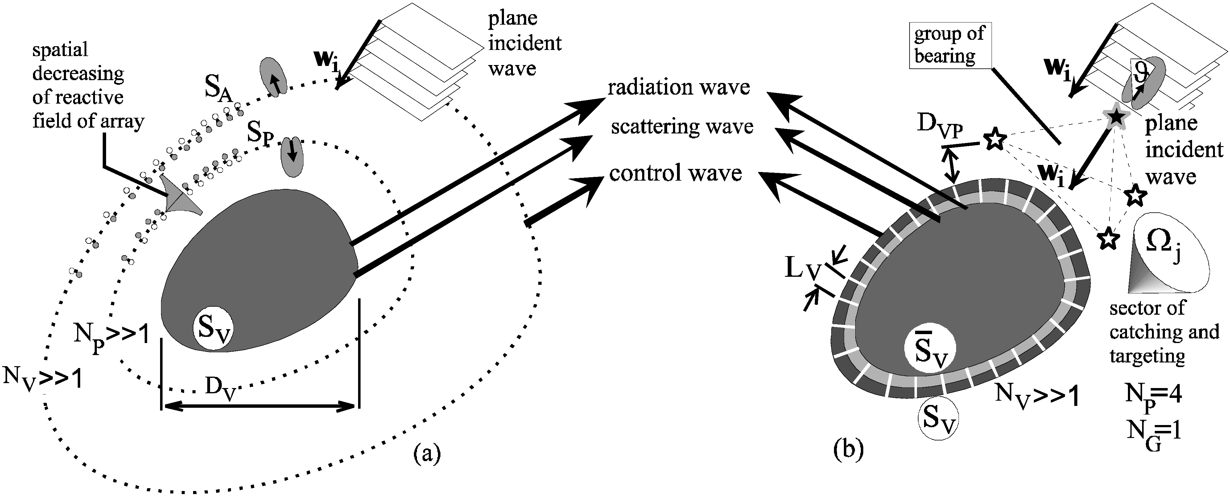
6. Suppression of the Scattering Field

Below we suggest an approach which requires a much smaller number of microphones and allows for placement of active sources immediately on the body’s surface, unlike those described in [24,25,26,27,28,29]. This active system consists of: (a) a subsystem of fast formation of a desired distribution of normal oscillatory velocities (DNOV) on the external surface of an active coating; (b) a subsystem of detection and targeting of incident waves. The active coating, described above, is spaced immediately on the surface of protected body. This coating creates the desired normal velocity (2) on external surface S_V.

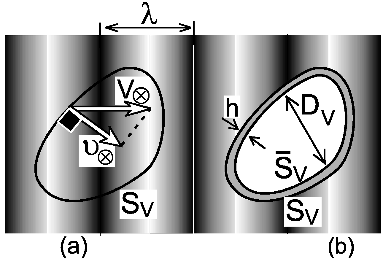
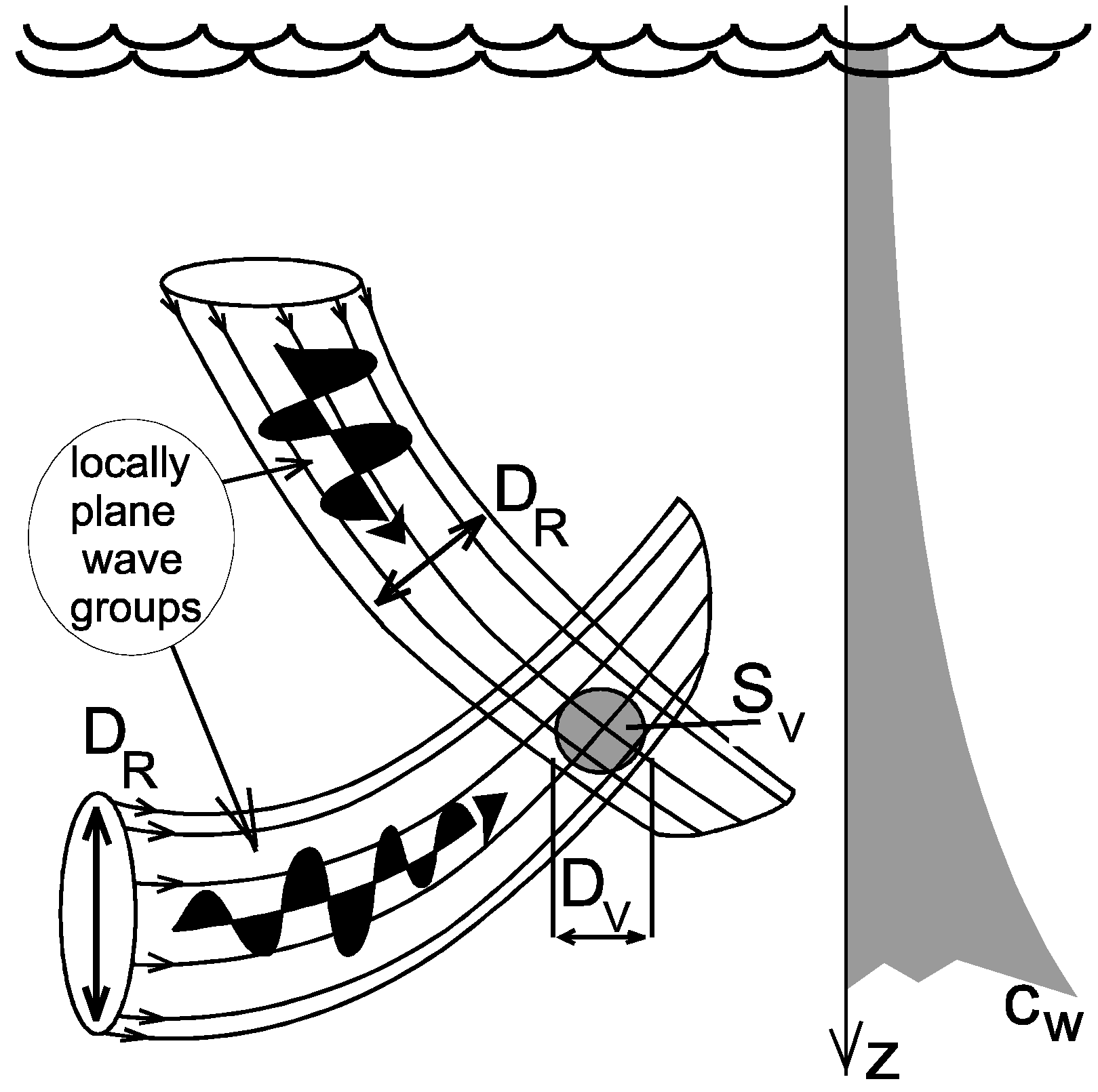
6.1. Incident Wave Field

We will use the following assumptions about the incident wave field. We consider the incident waves appearing, for example, as a result of ray-like (Figure 10) far propagation in the undersea sound channel [39]. We assume that the protected body (area) of characteristic size is fully covered by the cross section of tube of rays (of diameter ~D_R), i.e. D_R >> D_V. The wave within the tube of rays represents locally a running plane wave. The protected body can be spaced in the intersection of two (or more) tubes of rays and therefore the scattering problem can include two (or more) incident plane waves. We expect wave dispersion effects are very small, and speed of sound propagation is constant within the area occupied by the protected body.

Figure 10. The protected body in the intersection of two tubes of rays with two incident wave groups (locally plane). This is in the undersea acoustical channel with non-uniform distribution c_w(z) (along the depth z) of speed of propagation of acoustical waves.

Figure 10. The protected body in the intersection of two tubes of rays with two incident wave groups (locally plane). This is in the undersea acoustical channel with non-uniform distribution c_w(z) (along the depth z) of speed of propagation of acoustical waves.

The source of incident waves can radiate both video (without filling by sinusoidal shapes) pulses and radio-like sound pulses (with filling by sinusoidal shapes). In any case any video pulse will be converted via far propagation into a group of radio pulses, running along ray tubes. In addition we assume that each plane wave has finite duration. In other words each wave has a front border of plane shape moving with the speed of sound (of smooth or step-like shape), behind which the sound field is zero and also nonzero behind the border.

A step-like front border is more preferable for our approach, but it is impossible due to wave dispersion in long range propagation. The magnitudes of incident waves in the active acoustical detection problem (and in the absence of anti-sonar activity) must ensure the registration of scattered waves by the receiver system spaced on the same large distance between the scatterer (body) and the source of incident waves. Therefore if the distance between the source of incident waves and the protected body increases, the incident wave needs to shake the scatterer surface more powerfully for registration by the receiving microphones, without any increase of their sensitivity. This ensures the necessary accuracy of bearing and targeting (see below) of incident waves. Now we’ll assume that the incident waves represent a small number N_w > 1 of powerful, smooth, plane wave groups of finite duration and with amplitudes much greater than natural noise background σ_p of sound pressure. In the absence of a scattering body the sound pressure field of incident waves has the form:

$$p(\mathbf{r},t)=\underset{i=1}{\overset{N_w}{\Sigma }}{\Xi }_i[t-(\mathbf{r},{\mathbf{w}}_i)c_w^{-1}]$$

(18)

where i = 1,2,3,… N_w, (Figure 11b), $\{{\mathbf{w}}_i\}$-the normalized vectors of incident waves ($\left|{\mathbf{w}}_i\right|=1$), $c_w$- speed of sound propagation in the fluid, $(\mathbf{r},{\mathbf{w}}_i)$- scalar product of vectors.

6.2. The Scattering Suppression System and Algorithm

Let’s assume that a closed salient surface S_p (Figure 2a) surrounds the closed surface (outside surface of active coating of protected body). N_p small microphones with output signals p_m(t) of acoustical pressure are placed in the known points r = R_m of the surface S_p. At the output of the linear low pass filter without distortions and with frequency bandwidth ω_Q and with group delay τ_Q (the role of this filter is described in Section 6.3. below) we obtain $P_m(t)=\overline{Q}[p_m(t)]$.

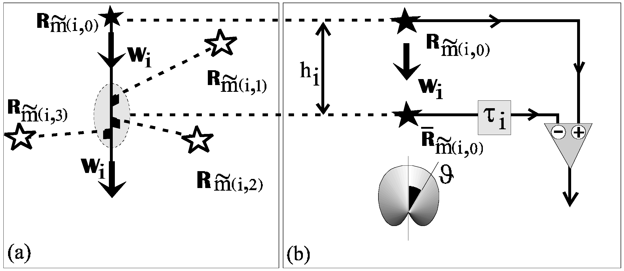
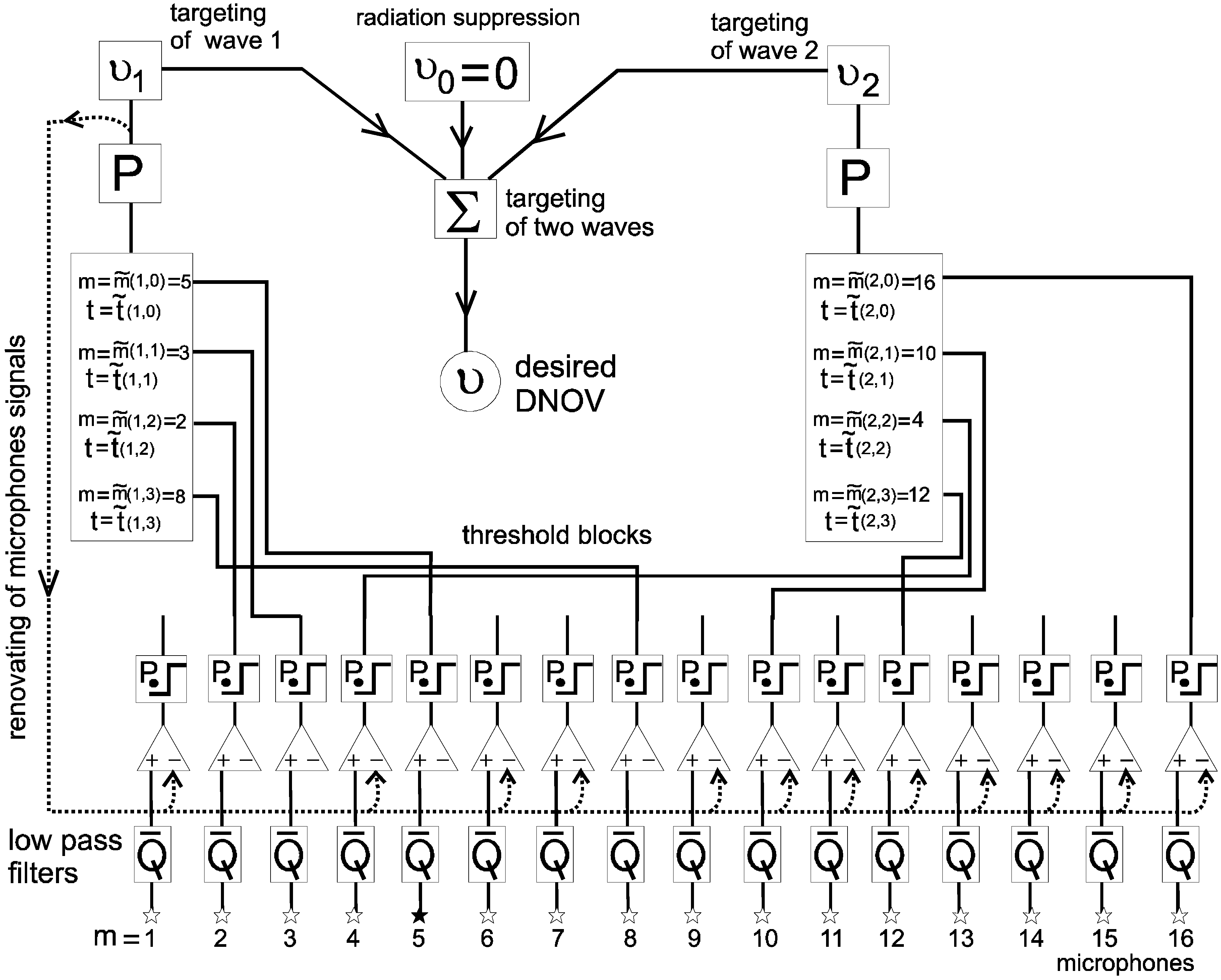
6.2.1. Targeting of One Incident Wave 

The first incident wave (with number i = 1) forms its bearing group, which consists of the four microphones (Figure 11a). These microphones differ from each other by their participation in the following events:

1. First contact between the front of an incident wave with any microphone on S_p means, that at this moment $t=\tilde{t}(1,0)$ (first for $\forall t\le \tilde{t}(1,0)$) on the microphone ★ with number $m=\tilde{m}(1,0)$ at the point $\mathbf{r}={\mathbf{R}}_{\tilde{m}(1,0)}$ the modulus $\left|\overline{Q}{\Xi }_1[t-(\mathbf{r},{\mathbf{w}}_1)c_w^{-1}\right|$ of the acoustical pressure $P_{\tilde{m}(1,0)}(t)$ of a first incident wave had crossed (from the bottom to the top) the threshold level $P_{•}$ of fixation, which satisfies the condition:

$${\mathsf{\sigma }}_P<<P_{•}<<{\left|{\Xi }_i\right|}_{\max }$$

(19)

2. 2-nd contact between front of an incident wave with any (another) microphone on S_p means, that at this moment $t=\tilde{t}(1,1)$ (first for $\forall t\le \tilde{t}(1,1)$) on the microphone ✫ with number $m=\tilde{m}(1,1)$ at the point $\mathbf{r}={\mathbf{R}}_{\tilde{m}(1,1)}$ the modulus $\left|\overline{Q}{\Xi }_1[t-(\mathbf{r},{\mathbf{w}}_1)c_w^{-1}\right|$ of the acoustical pressure $P_{\tilde{m}(1,1)}(t)$ of a first incident wave had crossed (from the bottom to the top) the threshold level $P_{•}$ of fixation.

3. 3-rd contact between front of an incident wave with any (another) microphone on S_p means, that at this moment $t=\tilde{t}(1,2)$ (firstly for $\forall t\le \tilde{t}(1,2)$) on the microphone ✫ with number $m=\tilde{m}(1,2)$ at the point $\mathbf{r}={\mathbf{R}}_{\tilde{m}(1,1)}$ the modulus $\left|\overline{Q}{\Xi }_1[t-(\mathbf{r},{\mathbf{w}}_1)c_w^{-1}\right|$ of acoustical pressure $P_{\tilde{m}(1,2)}(t)$ of a first incident wave had crossed (from the bottom to the top) with the threshold level $P_{•}$ of fixation.

Figure 11. Targeting of one (a) and three (b) incident waves. Incident wave (a) forms the bearing group of microphones (one title ★ microphone and three benchmark ✫ ones) on the surface S_p to match with the surface S_V of a protected body, covered by an active coating with pistons ${\overline{S}}_k$. Three incident waves (b), arriving from different directions ${\mathbf{w}}_1$, ${\mathbf{w}}_2$, ${\mathbf{w}}_3$ create three nonintersecting bearing groups.

Figure 11. Targeting of one (a) and three (b) incident waves. Incident wave (a) forms the bearing group of microphones (one title ★ microphone and three benchmark ✫ ones) on the surface S_p to match with the surface S_V of a protected body, covered by an active coating with pistons ${\overline{S}}_k$. Three incident waves (b), arriving from different directions ${\mathbf{w}}_1$, ${\mathbf{w}}_2$, ${\mathbf{w}}_3$ create three nonintersecting bearing groups.

4. 4-th contact between front of incident wave with any (another) microphone on S_p means, that at this moment $t=\tilde{t}(1,3)$ (firstly for$\forall t\le \tilde{t}(1,3)$) on the microphone ✫ with number $m=\tilde{m}(1,3)$ in the point $\mathbf{r}={\mathbf{R}}_{\tilde{m}(1,3)}$ the modulus $\left|\overline{Q}{\Xi }_1[t-(\mathbf{r},{\mathbf{w}}_1)c_w^{-1}\right|$ of acoustical pressure $P_{\tilde{m}(1,3)}(t)$ of a first incident wave had crossed (from the bottom to the top) with the threshold level $P_{•}$ of fixation.

The microphone ★ in the point ${\mathbf{R}}_{\tilde{m}(1,0)}$ we’ll call the title microphone with pressure signal $P_{\tilde{m}(1,0)}(t)$ and other microphones ✫ in the points ${\mathbf{R}}_{\tilde{m}(1,1)}$, ${\mathbf{R}}_{\tilde{m}(1,1)}$, ${\mathbf{R}}_{\tilde{m}(1,3)}$ we’ll call benchmark microphones with pressure signals $P_{\tilde{m}(1,1)}(t)$, $P_{\tilde{m}(1,2)}(t)$, $P_{\tilde{m}(1,3)}$ respectively. Taking into account the definitions 1-4, we obtain vector w₁ as a solution of the system of equations:

$$\{{\mathbf{w}}_1,({\mathbf{R}}_{\tilde{m}(1,k)}-{\mathbf{R}}_{\tilde{m}(1,0)})\}=[\tilde{t}(1,k)-\tilde{t}(1,0)]c_w,(k=1,2,3).$$

(20)

We assume, that all the microphones are very small (like points), therefore we can assume that the moments $t=\tilde{t}(1,0)$, $t=\tilde{t}(1,1)$, $t=\tilde{t}(1,2)$, $t=\tilde{t}(1,3)$ and the points ${\mathbf{R}}_{\tilde{m}(1,0)}$, ${\mathbf{R}}_{\tilde{m}(1,1)}$, ${\mathbf{R}}_{\tilde{m}(1,2)}$, ${\mathbf{R}}_{\tilde{m}(1,3)}$ must be mutually connected with each other, respectively, due to condition (19). In the absence of a protected body [or at condition (2)] the title microphone "knows" the incident wave field earlier than other microphones on the surface S_p. Knowing the wave pressure in the point ${\mathbf{R}}_{\tilde{m}(1,0)}$ and knowing the vector w₁, one can determine the incident wave field at the moment t in the point r, which satisfies the condition ${\mathbf{w}}_1(\mathbf{r}-{\mathbf{R}}_{\tilde{m}(1,0)})>0$, if we use the formula (which can be interpreted as the "diffraction" on the transparent body):

$${\Xi }_1(\mathbf{r},t)={\Xi }_1[{\mathbf{R}}_{\tilde{m}(1,0)},t-{\mathbf{w}}_1(\mathbf{r}-{\mathbf{R}}_{\tilde{m}(1,0)})c_w^{-1}]$$

(21)

Beginning from the moment $t=\tilde{t}(1,3)$, we are excluding the pressure of first incident wave in all microphones, which are not involved in a bearing group, targeting the first incident wave, i.e.:

$$P_m(t)=P_m(t)-P_{\tilde{m}(1,0)}(t-{\overline{\overline{\overline{\mathsf{\tau }}}}}_1)$$

(22)

where $m\ne \tilde{m}(1,j)$ (j = 0,1,2,3), ${\overline{\overline{\overline{\mathsf{\tau }}}}}_1=c_w^{-1}({\mathbf{w}}_1,{\mathbf{R}}_m-{\mathbf{R}}_{\tilde{m}(1,0)})$- scalar product of vectors. Due to operation (22) other microphones can register the arrival of the next incident waves.

6.2.2. Vector Microphone

To ensure the stability of active system we form a vector microphone (with selective directional pattern) with its direction of maximum sensitivity coinciding with the vector w₁ of the first incident wave, using the microphones of the bearing group, so we need two microphones, spaced on the axis w₁ at some distance h₁ from each other (Figure 12). At first we take the title microphone with output signal $P_{\tilde{m}(1,0)}(t)$. The signal ${\overline{P}}_{\tilde{m}(1,0)}(t)$ of the 2-nd microphone, which is spaced in some point ${\mathbf{R}}_{\tilde{m}(1,0)}+h_1{\mathbf{w}}_1$ (so far we only know that h1>0) will form a combination ${\overline{P}}_{\tilde{m}(1,0)}(t)=\mathsf{\mu }(1,1)P_{\tilde{m}(1,1)}(t)+\mathsf{\mu }(1,2)P_{\tilde{m}(1,2)}(t)+\mathsf{\mu }(1,3)P_{\tilde{m}(1,3)}(t)$ of signals of benchmark microphones ✫, where:

$$\mathsf{\mu }(1,1)+\mathsf{\mu }(1,2)+\mathsf{\mu }(1,3)=1, (\mathsf{\mu }(1,1),\mathsf{\mu }(1,2),\mathsf{\mu }(1,3)>0).$$

(23)

Figure 12. Forming of virtual vector microphone (b) with cardio directional pattern of sensitivity by means the combination (a) of signals of microphones group of bearing of the i-th incident wave. The mass center of points ${\mathbf{R}}_{\tilde{m}(1,1)}$, ${\mathbf{R}}_{\tilde{m}(1,2)}$, ${\mathbf{R}}_{\tilde{m}(1,3)}$ (with weights $\mathsf{\mu }(1,1)$, $\mathsf{\mu }(1,2)$, $\mathsf{\mu }(1,3)$) must be laying on the axis, coming from the point ${\mathbf{R}}_{\tilde{m}(i,0)}$ in direction of the vector w_i.

Figure 12. Forming of virtual vector microphone (b) with cardio directional pattern of sensitivity by means the combination (a) of signals of microphones group of bearing of the i-th incident wave. The mass center of points ${\mathbf{R}}_{\tilde{m}(1,1)}$, ${\mathbf{R}}_{\tilde{m}(1,2)}$, ${\mathbf{R}}_{\tilde{m}(1,3)}$ (with weights $\mathsf{\mu }(1,1)$, $\mathsf{\mu }(1,2)$, $\mathsf{\mu }(1,3)$) must be laying on the axis, coming from the point ${\mathbf{R}}_{\tilde{m}(i,0)}$ in direction of the vector w_i.

Ensuring the equation:

$${\mathsf{\mu }}_{(1,1)}{\mathbf{R}}_{\tilde{m}(1,1)}+{\mathsf{\mu }}_{(1,2)}{\mathbf{R}}_{\tilde{m}(1,2)}+{\mathsf{\mu }}_{(1,3)}{\mathbf{R}}_{\tilde{m}(1,3)}={\mathbf{R}}_{\tilde{m}(1,0)}+h_1{\mathbf{w}}_1$$

(24)

(i.e. center of masses $\mathsf{\mu }(1,1),\mathsf{\mu }(1,2),\mathsf{\mu }(1,3)$, spaced at points ${\mathbf{R}}_{\tilde{m}(1,1)}$, ${\mathbf{R}}_{\tilde{m}(1,2)}$, ${\mathbf{R}}_{\tilde{m}(1,3)}$ coincides with the point ${\mathbf{R}}_{\tilde{m}(1,0)}+h_1{\mathbf{w}}_1$) we obtain concrete weight coefficients $\mathsf{\mu }(1,1),\mathsf{\mu }(1,2),\mathsf{\mu }(1,3)$ and distance $h_1$. Taking into account the smoothness of the incident wave we form the signal ${\overline{P}}_{\tilde{m}(1,0)}(t)$ of the virtual microphone which is spaced at the point ${\overline{\mathbf{R}}}_{\tilde{m}(1,0)}={\mathbf{R}}_{\tilde{m}(1,0)}+h_1{\mathbf{w}}_1$. Now we obtain the output signal $U(t)=P_{\tilde{m}(1,0)}(t-{\mathsf{\tau }}_1)-{\overline{P}}_{\tilde{m}(1,0)}(t)$ (where ${\mathsf{\tau }}_1{h}_1/c_w$) of the vector microphone. For the wave running in direction $+{\mathbf{w}}_1$ (or $\mathsf{\vartheta }=0$, i.e. the first incident wave) the signal U(t) represents time derivative of sound pressure of incident wave in the point ${\mathbf{R}}_{\tilde{m}(1,0)}$ with delay ${\mathsf{\tau }}_1/2$: $U(t)\cong 2{\mathsf{\tau }}_1(d/dt)P_1[t-({\mathbf{R}}_{\tilde{m}(1,0)},{\mathbf{w}}_1)c_w^{-1}-({\mathsf{\tau }}_1/2)]$. The incident wave pressure $\Psi [t-({\mathsf{\tau }}_1/2)]$ in the point ${\mathbf{R}}_{\tilde{m}(1,0)}$ we obtain as integral ${\Psi }_{\tilde{m}(1,0)}[t-{({\mathsf{\tau }}_1/2)}^{-1}]={(2{\mathsf{\tau }}_1)}^{-1}{\displaystyle \underset{t^{\prime }=\tilde{t}(1,3)}{\overset{t^{\prime }=t}{\int }}U(t^{\prime })}d{t}^{\prime }$.

Below we will use the following symbols:

(a) ${\mathsf{\upsilon }}_i({\mathsf{\rho }}_k,t)$ - the desired normal velocity of the k-th active piston (temporally averaged on the interval T_V and spatially averaged along the external surface of piston S_k ), used in algorithm (25), when targeted to i-th incident wave (simultaneously at $i$ > 1) and $u_i({\mathsf{\rho }}_k,t)-u_i({\mathsf{\rho }}_k,t-T_V)=T_V{\mathsf{\upsilon }}_i({\mathsf{\rho }}_k,t)$ at $\tilde{t}(i,3)<t<\tilde{t}((i+1),0)$;

(b) ${\mathsf{\upsilon }}_0({\mathsf{\rho }}_k,t)$ -the desired normal velocity of $k$-th active piston before the arrival (or touch to microphone) of the first incident wave (averaged temporally on the interval $T_V$ and spatially along the external surface of piston $S_k$). In other words we have ${\mathsf{\upsilon }}_0({\mathsf{\rho }}_k,t)=0$, $u_0({\mathsf{\rho }}_k,t)=0$ in the problem of suppression of radiation by surface $S_V$ in the absence of incident waves i.e. if $t<\tilde{t}(1,0)$.

6.2.3. Renovation of DNOV on $S_V$ for the First Incident Wave

The desired velocity of $k$-th piston is [in accordance with (2)]:

$${\mathsf{\upsilon }}_1({\mathsf{\rho }}_k,t)={\mathsf{\upsilon }}_0({\mathsf{\rho }}_k,t)+{({\mathsf{\rho }}_w{c}_w{\mathsf{\sigma }}_k)}^{-1}{\displaystyle \underset{S_k}{\iint }d{S}_k}({\mathbf{w}}_1,\diamond ){\Psi }_{\tilde{m}(1,0)}(t-{\overline{\mathsf{\tau }}}_1),$$

where ${\overline{\mathsf{\tau }}}_1=c_w^{-1}({\mathbf{w}}_1,{\mathsf{\rho }}_k-{\mathbf{R}}_{\tilde{m}(1,0)})-({\mathsf{\tau }}_1/2)-{\mathsf{\tau }}_Q>0$, $({\mathbf{w}}_1,{\mathsf{\rho }}_k-{\mathbf{R}}_{\tilde{m}(1,0)})$ and $({\mathbf{w}}_1,\diamond )$ −scalar products of vectors. Simultaneously with the control processes, described above, the surface of the protected body (or internal surface ${\overline{S}}_V$ of active coating) oscillates with the same velocity, which must be without an active coating. DNOV is induced by two incident waves and internal sources of body vibrations. If we know exactly the microphones’ coordinates and exactly know the shape of the surface, then we can estimate the relative error $(\Delta \mathsf{\upsilon }/\mathsf{\upsilon })$ of DNOV as the following expression:

$$(\Delta \mathsf{\upsilon }/\mathsf{\upsilon })\approx {(\Delta P/P)}^2({\mathsf{\lambda }}_{\max }{D}_V/{\mathsf{\ell }}_P^2),$$

(25)

where ${\mathsf{\ell }}_P$-characteristic distance between adjacent microphones in group of bearing, ${\mathsf{\lambda }}_{\max }$-maximum length of the waves to be damped, $(\Delta P/P)$-relative error of the measured acoustical pressure. The formula (25) can be used as the rough simple estimate of the relative value of the residual acoustical scattered field. The magnitude $B_{n,k}$ of signal of excitation of k-th piston of active coating at the moment $t=n{T}_V$ is in accordance with algorithm (15), determined by the formula $B_{n,k}={({\mathsf{\psi }}_0{T}_V/2)}^{-1}{\displaystyle \underset{n{T}_V-T_V}{\overset{n{T}_V}{\int }}}\overline{F}[Y_k(t)-{\mathsf{\upsilon }}_1({\mathsf{\rho }}_k,n{T}_V)]dt$, where $Y_k(t)$-current value (measured) spatially averaged along the k-th active piston, ${\mathsf{\upsilon }}_1({\mathsf{\rho }}_k,n{T}_V)$ -the desired velocity of the k-th piston.

6.2.4. Microphone Signal Renovation for Catching the Second Incident Wave.

To prepare other microphones with numbers $m\ne \tilde{m}(1,j)$ ($j=0,1,2,3$ ) for registration and targeting of next waves (beginning from the moment $t=\tilde{t}(1,0)$) we exclude acoustical pressure of the first incident wave, i.e.

$$P_m(t)=P_m(t)-{\Psi }_{\tilde{m}(1,0)}(t-{\overline{\overline{\mathsf{\tau }}}}_1),$$

(26)

where ${\overline{\overline{\mathsf{\tau }}}}_1=c_w^{-1}({\mathbf{w}}_1,{\mathbf{R}}_m-{\mathbf{R}}_{\tilde{m}(1,0)})-({\mathsf{\tau }}_1/2)-{\mathsf{\tau }}_Q$ …etc.

Figure 13. The example of forming groups of bearing for renovation of signals of microphones for $N_P=16$.

Figure 13. The example of forming groups of bearing for renovation of signals of microphones for $N_P=16$.

So the first incident wave is described by the following group of numbers and vectors (Figure 13): {$\tilde{t}(1,0)$, $\tilde{m}(1,0)$, ${\mathbf{R}}_{\tilde{m}(1,0)}$}, {$\tilde{t}(1,1)$, $\tilde{m}(1,1)$, ${\mathbf{R}}_{\tilde{m}(1,1)}$}, {$\tilde{t}(1,2)$, $\tilde{m}(1,2)$, ${\mathbf{R}}_{\tilde{m}(1,2)}$}, {$\tilde{t}(1,3)$, $\tilde{m}(1,3)$, ${\mathbf{R}}_{\tilde{m}(1,3)}$}, ${\mathbf{w}}_1$, {$\mathsf{\mu }(1,1)$, $\mathsf{\mu }(1,2)$, $\mathsf{\mu }(1,3)$}, $h_1$, ${\mathsf{\tau }}_1$, ${\mathsf{\tau }}_Q$. Here $\tilde{t}(i,j)$, $\tilde{m}(i,j)$, $\mathsf{\mu }(i,j)$−functions of discrete arguments $i=1,2,\dots ,N_w$, $j=0,1,2,3$; $\tilde{t}(i,j)$−real number, а $\tilde{m}(i,j)$−whole number.

Now we remind the sense of the used symbols: k = 1,2,…,N_V - ordinal numbers of damping pistons; $n=0,1,2,\dots$- ordinal number of basic temporal cycle (of duration T_V) of active system; $i=1,2,3,\dots ,N_w$ - ordinal numbers of incident waves in sequence of their first contacts (touching) with microphones system; $j=0,1,2,3$ -ordinal numbers of microphones in the group of bearing of the $i$-th incident wave in dependence of concrete scenario; $m=1,2,3,....,N_P$ -ordinal numbers of "physical" microphones independently of any scenario. Let’s assume that system of incident waves (18) and microphones coordinates Rm ensure the following conditions: $\tilde{t}(i,0)\le \tilde{t}(i,1)\le \tilde{t}(i,2)\le \tilde{t}(i,3)$, for$\forall i$, R(_i,k) ≠ R(j_,k) for $\forall i\ne j$ and $\forall k=0,1,2,3$, $T_V$<<$\left|\tilde{t}(i,1)-\tilde{t}(i,0)\right|$,$\left|\tilde{t}(i,2)-\tilde{t}(i,1)\right|$,$\left|\tilde{t}(i,3)-\tilde{t}(i,2)\right|$<$D_{VP}/c_w$. In other words we assume that the microphone system and system of incident waves always permit us to form bearing groups without intersection of microphones for targeting each incident wave.

6.2.5. Two Incident Wave Targeting

At the moment $t=\tilde{t}(2,0)$ the second incident wave arrives Figure 11-b). Among a lot of microphones with numbers $m\ne \tilde{m}(1,j)$ (where $j=0,1,2,3$) we elect one title microphone ★ and three bench-mark microphones ✫, forming the group of bearing in accordance with the rule (above described) of first crossing (from the bottom to the top) of threshold level $P_{•}$ (Figure 13) by the modulus $\left|{\Xi }_2[t-(\mathbf{r},{\mathbf{w}}_2)c_w^{-1}\right|$ of acoustical pressure of 2-nd incident wave on the moments $t=\tilde{t}(2,0)$, $t=\tilde{t}(2,1)$, $t=\tilde{t}(2,2)$, $t=\tilde{t}(2,3)$. We assume, that these moments are connected with front border of second incident wave in the spatial points ${\mathbf{R}}_{\tilde{m}(2,0)}$, ${\mathbf{R}}_{\tilde{m}(2,1)}$, ${\mathbf{R}}_{\tilde{m}(2,2)}$, ${\mathbf{R}}_{\tilde{m}(2,3)}$ respectively. From the system of equations:

$$\{{\mathbf{w}}_2,({\mathbf{R}}_{\tilde{m}(2,k)}-{\mathbf{R}}_{\tilde{m}(2,0)})\}=[\tilde{t}(2,k)-\tilde{t}(2,0)]c_w, (k=1,2,3).$$

(27)

we obtain the vector of 2-nd incident wave. From the time $t=\tilde{t}(2,0)$ up to time $t=\tilde{t}(2,3)$ we cancel acoustical pressure of the 1-st incident wave in all microphones, if they are not included in the group of bearing, to target on both 1-st and 2-nd incident waves, i.e.:

$$P_m(t)=P_m(t)-P_{\tilde{m}(2,0)}(t-{\overline{\overline{\overline{\mathsf{\tau }}}}}_2),$$

(28)

where $m\ne \tilde{m}(1,j),\tilde{m}(2,j)$ ($j=0,1,2,3$), ${\overline{\overline{\overline{\mathsf{\tau }}}}}_2=c_w^{-1}({\mathbf{w}}_2,{\mathbf{R}}_m-{\mathbf{R}}_{\tilde{m}(2,0)})$. Due to operation (28) other microphones (they are not involved in any group of bearing formed already) can register the arrival of next incident waves. In the absence of scattering body (or at condition (2)) the title microphone "knows" incident wave field before other microphones on surface $S_P$. Knowing the wave pressure in the point ${\mathbf{R}}_{\tilde{m}(2,0)}$ and knowing the vector ${\mathbf{w}}_2$, one can determine the incident wave field at the moment $t$ in the point $\mathbf{r}$, which satisfy the condition $({\mathbf{w}}_2,(\mathbf{r}-{\mathbf{R}}_{\tilde{m}(2,0)}))>0$. We obtain this from the formula

$${\Xi }_2(\mathbf{r},t)={\Xi }_2[{\mathbf{R}}_{\tilde{m}(2,0)},t-{\mathbf{w}}_2(\mathbf{r}-{\mathbf{R}}_{\tilde{m}(2,0)})c_w^{-1}].$$

(29)

As in the procedure of the vector microphone, described above, we form the signal $P_{\tilde{m}(2,0)}(t-{\mathsf{\tau }}_2)$ and then form signal ${\overline{P}}_{\tilde{m}(1,0)}(t)$ of the view ${\overline{P}}_{\tilde{m}(2,0)}(t)=\mathsf{\mu }(2,1)P_{\tilde{m}(2,1)}(t)+\mathsf{\mu }(2,2)P_{\tilde{m}(2,2)}(t)+\mathsf{\mu }(2,3)P_{\tilde{m}(2,3)}(t)$. The parameters μ(2,1), μ(2,2), μ(2,3),h₂(μ(2,1),μ(2,2),μ(2,3)>0), we obtain from the system of equations:

$$\mathsf{\mu }(2,1)+\mathsf{\mu }(2,2)+\mathsf{\mu }(2,3)=1 ,$$

(30)

$${\mathsf{\mu }}_{(2,1)}{\mathbf{R}}_{\tilde{m}(2,1)}+{\mathsf{\mu }}_{(2,2)}{\mathbf{R}}_{\tilde{m}(2,2)}+{\mathsf{\mu }}_{(2,3)}{\mathbf{R}}_{\tilde{m}(2,3)}={\mathbf{R}}_{(2,0)}+h_2{\mathbf{w}}_2$$

(31)

The output signal of vector microphone has the form ${\Psi }_{\tilde{m}(2,0)}[t-{({\mathsf{\tau }}_2/2)}^{-1}]={(2{\mathsf{\tau }}_2)}^{-1}{\displaystyle \underset{t^{\prime }=\tilde{t}(2,3)}{\overset{t^{\prime }=t}{\int }}U(t^{\prime })}d{t}^{\prime }$, where ${\mathsf{\tau }}_2=h_2/c_w$, $U(t)=P_{\tilde{m}(2,0)}(t-{\mathsf{\tau }}_2)-{\overline{P}}_{\tilde{m}(2,0)}(t)$.

6.2.6. Renovation of DNOV on $S_V$ for Two Incident Waves

The desired velocity of the k-th piston is [in accordance with (2)]:

$${\mathsf{\upsilon }}_2({\mathsf{\rho }}_k,t)={\mathsf{\upsilon }}_1({\mathsf{\rho }}_k,t)+{({\mathsf{\rho }}_w{c}_w{\mathsf{\sigma }}_k)}^{-1}{\displaystyle \underset{S_k}{\iint }d{S}_k}({\mathbf{w}}_2,\diamond ){\Psi }_{\tilde{m}(2,0)}(t-{\overline{\mathsf{\tau }}}_2),$$

where ${\overline{\mathsf{\tau }}}_2=c_w^{-1}({\mathbf{w}}_2,{\mathsf{\rho }}_k-{\mathbf{R}}_{\tilde{m}(2,0)})-({\mathsf{\tau }}_2/2)-{\mathsf{\tau }}_Q>0$, $({\mathbf{w}}_2,{\mathsf{\rho }}_k-{\mathbf{R}}_{\tilde{m}(2,0)})$, $({\mathbf{w}}_2,\diamond )$ −scalar products of vectors. Simultaneously with the control processes, described above, the surface of the protected body (or internal surface ${\overline{S}}_V$ of an active coating) oscillates with the same velocity, which must be without active coating. DNOV is induced by two incident waves and internal sources of vibrations of body. The magnitude $B_{n,k}$ of signal of excitation of $k$-th piston of active coating at the moment $t=n{T}_V$ is in accordance with algorithm (15) is determined by the formula $B_{n,k}={({\mathsf{\psi }}_0{T}_V/2)}^{-1}{\displaystyle \underset{n{T}_V-T_V}{\overset{n{T}_V}{\int }}}\overline{F}[Y_k(t)-{\mathsf{\upsilon }}_2({\mathsf{\rho }}_k,n{T}_V)]dt$, where $Y_k(t)$-current value (measured) spatially averaged along the $k$-th active piston, ${\mathsf{\upsilon }}_2({\mathsf{\rho }}_k,n{T}_V)$ -the desired velocity of $k$-th piston.

6.2.7. Microphone Signal Renovation for Catching the Third Incident Wave

To prepare other microphones with numbers $m\ne \tilde{m}(1,j),\tilde{m}(2,j)$ ($j=0,1,2,3$) for registration and targeting of subsequent waves (beginning from the moment $t=\tilde{t}(2,0)$) we exclude acoustical pressure of the second incident wave, i.e. $P_m(t)=P_m(t)-{\Psi }_{\tilde{m}(2,0)}(t-{\overline{\overline{\mathsf{\tau }}}}_2)$, where ${\overline{\overline{\mathsf{\tau }}}}_2=c_w^{-1}({\mathbf{w}}_2,{\mathbf{R}}_m-{\mathbf{R}}_{\tilde{m}(2,0)})-({\mathsf{\tau }}_2/2)-{\mathsf{\tau }}_Q$ …etc.

6.2.8. Calibration

To ensure the accuracy of our measurement of acoustical pressure $p(\mathbf{r},t)$, we need to have identical calibration within each bearing group. We assume that the output of each microphone depends linearly on acoustical pressure: $P_m(t)=a_m{p}_m(t)+b_m$ ($m=1,2,\dots ,N_P$). Coefficients $a_m$, $b_m$ have slow temporal drift and need fast identification of them. The relation (like (18), (21), (29)) between time delay and media particle displacement is constant along the propagation of front plane border of wave. These relations give us parameters a_m, bm,…, if the coordinates of microphones are known exactly and natural acoustical noise is very weak in comparison with the incident waves.

6.2.9. Reset of Active System

If at some moment we notice, that the "silence" (i.e.$\left|P_m(t)\right|<P_{•}$ ) has been continued simultaneously on each microphone of some group of bearing during the time $~L_P/c_w$ (without exclusions), so the microphones of this group of bearing should be returned to their initial status (i.e. waiting) and do not control active coating. In other words every moment $t=n{T}_V$ the active system is checking the output of the counter$I_i(t_n)=N_0^{-1}\underset{\mathsf{\ell }=n-N_0}{\overset{\mathsf{\ell }=n}{\Sigma }}\underset{\begin{array}{l}m=\tilde{m}(i,k)\\ k=0,1,2,3\end{array}}{\Pi }I\left(\left|P_{\tilde{m}(i,k)}(t_{\mathsf{\ell }})\right|-P_{•}\right)$ for each $i$>-th group of bearing (where $N_0=L_P/c_w$ , $I(\mathsf{\xi })=0$ at $\mathsf{\xi }<0$ , $I(\mathsf{\xi })=1$ at $\mathsf{\xi }\ge 0$ ). The signal of i-th group of bearing resets the waiting status, when gets jump from position I_i = 1 into position I_i = 0.

6.3. Notes about the Stability of an Active System with Microphones

The description above was made under the assumption that active coating forms desired DNOV on the surface S_V sufficiently quickly, precisely and safely. Now we consider possible instability channels, created by microphones. Together these channels must cover all frequencies. Only in this case their blocking could guarantee system’s stability. There the three channels can generate instability via microphones.

1. Active coating generates the acoustical field in the range (3) and this field penetrates via microphones. This channel of instability is blocked by the vector-microphone, which ensures the feedback coefficient has a value of less than 1.

2. Active coating generates the sound field outside of the range (3) too. On these frequencies the directional pattern of vector-microphone has too many of narrow petals, but does not ensure the desired integral (in body angle $\pm 2\mathsf{\pi }$) and anisotropy with respect to the vector ${\mathbf{w}}_i$ of incident wave, if $h_i\mathsf{\omega }/c_w>>1$, for instance. Besides this, it is impossible to form the desired DNOV by pistons of finite dimension $L_V$. To block this channel of instability we use low pass filter with time constant ${\mathsf{\tau }}_Q$ (under the condition $D_V<<c_w{\mathsf{\tau }}_Q<<2\mathsf{\pi }/{\mathsf{\chi }}_{\max }$) on the output of each microphone without inertial distortions of desired signals and inserting of only delay ${\mathsf{\tau }}_Q$. Control system takes into account this delay without problems with targeting of incident wave with condition ${\mathsf{\tau }}_Q<D_{VP}/c_w$.

3. Reactive acoustical field (near field), created by active coating in the range (3), penetrates the microphones too. This field can’t be reduced by a vector microphone. However this field is exponentially decreasing as $\mathsf{\gamma }=\exp \left[-D_{VP}\sqrt{{(2\mathsf{\pi }/L_V)}^2-{\mathsf{\chi }}_{\max }^2}\right]$ at the distance $D_{VP}$ from coating. So at not very large distance $D_{VP}$ we can get $\mathsf{\gamma }<<1$ by decreasing L_V.

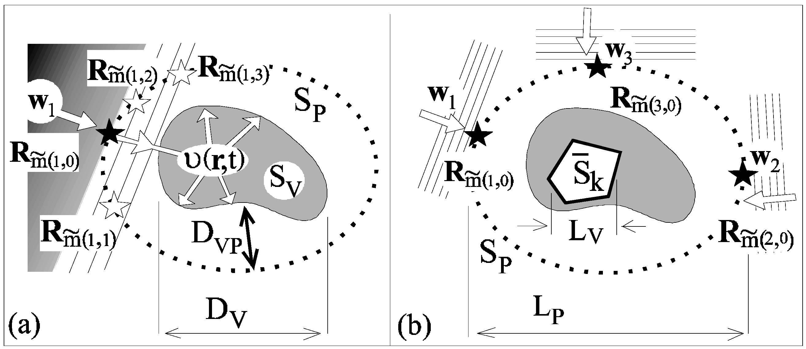
6.4. Hierarchy of Scales in the System of Scattering Suppression

Summarizing the above considered, we can state, that, to ensure stability and efficiency of active system with microphones (if the stability and efficiency of system of synthesis of DNOV on $S_V$ was earlier ensured (18)), we must satisfy the following conditions:

$$D_{VP}/c_w>{\mathsf{\tau }}_Q>>T_V, \exp \left[-D_{VP}\sqrt{{(2\mathsf{\pi }/L_V)}^2-{\mathsf{\chi }}_{\max }^2}\right]<<1, L_V{\mathsf{\chi }}_{\max },{\mathsf{\ell }}_P{\mathsf{\chi }}_{\max }.$$

(32)

6.5. Placement of Microphones

Now we will consider questions of rational placement of microphones, which allows us to target the required number N_w of incident waves with a minimum number of microphones. Each i-th bearing group is targeting only one incident wave. We characterize this group by its targeting and catching sector Ω_j. The last one represents multitude Ω_j of directions ${\mathbf{w}}_i$ of incident waves. The i-th bearing group can target only one incident wave (with ${\mathbf{w}}_i\in {\Omega }_j$) till first contact of this wave with the protected body. In other words it presents a lot of directions for which one bearing group could form a vector-microphone or solve the system of equations (7), (12) with sufficient accuracy.

Figure 14. Placment of microphones on the surface of prominent hexagonal polyhedron $S_P$ near its apexes. $S_{ji1}$, $S_{ji2}$,$S_{ji3}$-the sides of $S_P$ closing to its $j$-th apex with $i$-th group of bearing with sector ${\Omega }_i$ for catching and target of $i$-th incident wave. Planes ${\overline{S}}_{ji12}$, ${\overline{S}}_{ji31}$, ${\overline{S}}_{ji32}$-bisectors of angles between sides $S_{ji1}$ and $S_{ji2}$, $S_{ji3}$ and $S_{ji1}$, $S_{ji3}$ and $S_{ji2}$. Title microphone ★ is spaced in $i$-th apex of $S_P$, benchmark microphones ✫ are spaced on planes ${\overline{S}}_{ji12}$, ${\overline{S}}_{ji31}$, ${\overline{S}}_{ji32}$. Here we assumed $j$-ordinal number of apex, $i$- ordinal number of incident wave (in order of their arrival).

Figure 14. Placment of microphones on the surface of prominent hexagonal polyhedron $S_P$ near its apexes. $S_{ji1}$, $S_{ji2}$,$S_{ji3}$-the sides of $S_P$ closing to its $j$-th apex with $i$-th group of bearing with sector ${\Omega }_i$ for catching and target of $i$-th incident wave. Planes ${\overline{S}}_{ji12}$, ${\overline{S}}_{ji31}$, ${\overline{S}}_{ji32}$-bisectors of angles between sides $S_{ji1}$ and $S_{ji2}$, $S_{ji3}$ and $S_{ji1}$, $S_{ji3}$ and $S_{ji2}$. Title microphone ★ is spaced in $i$-th apex of $S_P$, benchmark microphones ✫ are spaced on planes ${\overline{S}}_{ji12}$, ${\overline{S}}_{ji31}$, ${\overline{S}}_{ji32}$. Here we assumed $j$-ordinal number of apex, $i$- ordinal number of incident wave (in order of their arrival).

6.5.1. Geometry of the Microphone Grid 

Numerous microphone placement variants are possible. Below we’ll describe only one concrete version. In this version the surface S_p is represented by a prominent hexagonal polyhedron with plane six cornered sides (Figure 14) of characteristic linear scale $D_P$ and apexes with ordinal number $j=1,2,3,\dots ,N_w$. Each group of bearing is spaced near polyhedron’s apexes. Title microphone ★ of $i$-th group of bearing is spaced in $j$-th apex which unites three sides $S_{ji1}$, $S_{ji2}$, $S_{ji3}$. Planes ${\overline{S}}_{ji12}$, ${\overline{S}}_{ji31}$, ${\overline{S}}_{ji32}$ are bisectors of angles between sides $S_{ji1}$ and $S_{ji2}$, $S_{ji3}$ and $S_{ji1}$, $S_{ji3}$ and $S_{ji2}$ respectively. Benchmark microphones ✫ are spaced on planes ${\overline{S}}_{ji12}$, ${\overline{S}}_{ji31}$, ${\overline{S}}_{ji32}$. Distances $D_{ji12}$, $D_{ji23}$, $D_{ji31}$ do not exceed quarter of corresponding $S_P$’s edges. Lines $d_{ji12}$, $d_{ji23}$, $d_{ji31}$ are normal with corresponding edges of $S_P$ and spaced in planes ${\overline{S}}_{ji12}$, ${\overline{S}}_{ji31}$, ${\overline{S}}_{ji32}$ correspondingly. Small (but finite) values $d_{ji12}~D_{ji12}^2/R_P<D_{ji12}$, $d_{ji23}~D_{ji23}^2/R_P<D_{ji23}$, $d_{ji31}~D_{ji31}^2/R_P<D_{ji31}$ are necessary to ensure targeting of incident wave, when its direction is normal to some side $S_{ji1}$, $S_{ji2}$, $S_{ji3}$ of $S_P$. Besides this, the finite distances $d_{ji12}$, $d_{ji23}$, $d_{ji31}>0$ are necessary to ensure sufficient accuracy of the solution of equations (20), (23), (24), (27), (30), (31). $R_P$ denotes the averaged curvature radius of $S_P$ (i.e. curvature radius of some smooth surface embracing $S_P$ closely). We choose concrete values $D_{ji12}$, $D_{ji23}$, $D_{i31}$, $d_{ji12}$, $d_{ji23}$, $d_{i31}$ to ensure: (a) covering of the full area of directions ${\mathbf{w}}_i$ of possible arrival of incident waves; (b) simultaneous targeting of several incident waves by several groups of bearing without any conflicts between each other. Total number $N_P$ of microphones, number $N_{SP}$ of apexes of polyhedron $S_P$, total number $N_{PG}$ of groups of bearing, total number $N_w$ (expected) of incident waves simultaneously targeted are connected by relation $N_P/4=N_{PG}=N_{SP}=N_w$. The distance $D_P$ between adjacent title microphones in any area of surface $S_P$ with curvature radius $R_P$ one can estimate approximately as $D_P\le 2R_P{\mathsf{\theta }}_w$, where $R_P$ refers to some smooth surface embracing all apexes of $S_P$. There ${\mathsf{\theta }}_w$ denotes the expected minimum difference between directions of incident waves, i.e. ${\mathsf{\theta }}_w=\underset{n\ne m}{\min }[\arccos ({\mathbf{w}}_n,{\mathbf{w}}_m)]$ ($n,m=1,2,\dots ,N_w$).

Figure 15. An example of prominent hexagonal polyhedron surface $S_P$ embracing the protected surface $S_V$ of sufficiently stretched shape. Microphones are concentrated only near apexes of polyhedron $S_P$ (number of bearing groups is equal to the number of apexes of $S_P$) in the end areas of $S_P$. Microphones are absent in the lateral area of $S_P$, where its curvature (along the longitudinal coordinate) is zero.

Figure 15. An example of prominent hexagonal polyhedron surface $S_P$ embracing the protected surface $S_V$ of sufficiently stretched shape. Microphones are concentrated only near apexes of polyhedron $S_P$ (number of bearing groups is equal to the number of apexes of $S_P$) in the end areas of $S_P$. Microphones are absent in the lateral area of $S_P$, where its curvature (along the longitudinal coordinate) is zero.

6.5.2. Total Number of Microphones

One can see, that in the areas of S_p with smaller curvature radius R_p the density of microphones is larger, than in the areas of S_p with larger curvature radius S_p. It is the most obviously in the case of surface S_p (and S_V) of stretched shape (Figure 15) with length $L_P$ and curvature radius $R_P<<L_P$ at its ends. The microphones are absent on the side areas of surface $S_P$ due to our assumption about plane incident waves. In other words, our active system protects directions in space, unlike protection of areas of space in the traditional systems. When our active system targets $N_w\approx 4\mathsf{\pi }/{\mathsf{\theta }}_w^2>>1$ incident waves, using our approach, the active system needs $N_P\approx 16\mathsf{\pi }/{\mathsf{\theta }}_w^2$ microphones. This amount is smaller by $N_P/N_{P0}\approx {\mathsf{\lambda }}_{\min }^2/{\mathsf{\theta }}_w^2{L}_P{R}_P$ times than when using the approach of G.D. Malyuzhinets.

6.6. Microphone Noise

By the reduction of the number of microphones included in the control of the active coating, we reduce the total power of control noise $N_{P0}/N_P>>1$ times. This noise can be significantly less than in the case, where we are targeting all $N_w\approx 4\mathsf{\pi }/{\mathsf{\theta }}_w^2$ expected incident waves simultaneously (i.e. all microphones are involved in control). Really the number ${\overline{N}}_w<<N_w$ of incident waves can be much less (for example${\overline{N}}_w=1$ or ${\overline{N}}_w=2$). In this real case the system suggested can give the reducing of total power of control noise in $(N_{P0}/N_P)(N_w/{\overline{N}}_w)>>1$ times, at comparing with the method of G.D. Malyuzhinets. Of course we assume that microphone noises are statistically independent with zero mean value, and power of sum of noises is equal to sum of noise powers of each microphone. And this sum of noise powers does not depend of signs, with which these noises are included in sum with signals.

6.6.1. Noise of a Vector Microphone

The spatial base $h_i<<{\mathsf{\lambda }}_{\max }$ (Figure 12) of vector microphones is of the order $h_i~{{\mathsf{\ell }}^2}_P{R}_P$. The output signal of the vector microphone represents the differential between two signals and has characteristic magnitude $\Psi ~P{h}_i{\mathsf{\lambda }}_{\max }^{-1}$, where $P$- characteristic magnitude of incident wave pressure. We need a small relative control error ${\mathsf{\sigma }}_P/\Psi$, where ${\mathsf{\sigma }}_P$ - square noise value or square root of mean power of noise. We use the assumption about large magnitude of incident wave to have ${\mathsf{\sigma }}_P/\Psi <<1$. So we need ensure the condition ${\mathsf{\sigma }}_P/P<<h_i{\mathsf{\lambda }}_{\max }^{-1}$, which is analogous to (19).

7. Conclusions

Above we considered the solution in the form of active system with the qualitative characteristics (a-d), presented in the beginning of Section 2. Among all methods and systems, presented in the introduction (Section 1), the demands (a-c) can be satisfied simultaneously only by method of G. D. Malyuzhinets (Figure 16a, where S_A, S_p - radiating and receiving Huygens’ surfaces) and the method which was suggested in this paper (Figure 16b).

Below we will show more thoroughly the differences (advantages and drawbacks) between these two approaches. Let’s assume that incident field presents the plane wave with direction w_i inside the sector ${\Omega }_i$ (Figure 16b, of catching and targeting, see Section 6.1). The approach suggested requires only four microphones, unlike Malyuzhinets’ method, where N_P >>1 (see Section 6.5.2). In both cases (Figure 16a,b) the bodies have vibrations (caused by internal sources and incident waves) as in the absence of an active system. Active control by four microphones (bearing group, Figure 16b) gives much smaller control noises than in Maliuzhinets’ method (see Section 6.6). In addition, the means of the fastening of the four microphones are greatly more transparent (transparency is necessary), than the microphones array in Malyuzhinets’ method. In both approaches the total amount of actuators (active pistons) is very high N_V>>1. However, Malyuzhinets’ method does not permit placement of actuators immediately on the protected body (to keep their unidirectional characteristics), and this leads to the great technical problem of transparent fastening thereof.

Figure 16. Comparison of method of G.D. Malyuzhinets (a) with the simplest version of the suggested system (b).

Figure 16. Comparison of method of G.D. Malyuzhinets (a) with the simplest version of the suggested system (b).

This paper represents an attempt at solving the edge problem of active wave suppression under initial conditions. Such a problem statement (plus stable promotion of technological developments of very fast, very small and highly accurate elements of hard electronics) gave several new possibilities to find the solutions, more close to practice, if the conditions (18), (32) are fulfilled.

References and Notes

1. Rozanov, N.N. Invisibility: “pro” and “contra”. Priroda 2008, 6, 3–10. [Google Scholar]
2. Bobrovnitski, Yu.I. A nonscattering coating for a cylinder. Acoustical Physics 2008, 6, 879–889. [Google Scholar] [CrossRef]
3. Alu, A.; Engheta, N. Achieving transparency with plasmonic and metamaterial coatings. Physical Review 2005, E72, 0166623. [Google Scholar]
4. Shurig, D.; Mock, J.; Justice, B.; Cummer, S.; Pendry, J.; Starr, A.; Smith, D. Metamaterial electromagnetic cloak at microwave frequencies. Science 2006, 314, 977–980. [Google Scholar] [CrossRef] [PubMed]
5. Torrent, D.; Sanchez-Dehesa, J. Acoustic metamaterials for two-dimensional sonic devices. New Journal of Physics 2007, 9, 323–335. [Google Scholar] [CrossRef]
6. Kerker, M. Invisible bodies. Journal of the Optical Society of America 1975, 65, 376–379. [Google Scholar] [CrossRef]
7. Cummer, S.A.; Popa, B.I.; Shuring, D.; Smith, D.R.; Pendry, J.; Rahm, M.; Starr, A. Scattering theory derivation of a 3D acoustic cloaking shell. Physical Review Letter 2008, 100, 024301. [Google Scholar] [CrossRef]
8. Leonhard, U. Notes on conformal invisibility devices. New Journal of Physics 2006, 8, 118–123. [Google Scholar] [CrossRef]
9. Jessel, M.; Mangiante, G. Active sound absorbers in an air ducts. Sound and Vibration 1973, 6, 383–390. [Google Scholar] [CrossRef]
10. Zhu, H.; Raymany, R; Stelson, K.A. Active control of acoustic reflection, absorption and transmission using thin panel speakers. Journal of the Acoustical Society of America 2003, 2, 852–870. [Google Scholar] [CrossRef]
11. Elliott, S.J.; Joseph, P.; Nelson, P.A.; Johnson, M.E. Active output absorption in the active control sound. Journal of the Acoustical Society of America 1993, 5, 2501–2512. [Google Scholar]
12. Premount, A. Vibration Control of Active Structures, an Introduction; Kluwer Academic Publishers: New York, NY, USA, 2002. [Google Scholar]
13. Fuller, C.R.; Elliott, S.J.; Nelson, P.A. Active Control of Vibration; Academic Press: London, UK, 1996. [Google Scholar]
14. Nelson, P.A.; Elliott, S.J. Active control of Sound; Academic Press: London, UK, 1993. [Google Scholar]
15. Furstoss, M.; Thenail, D.; Galland, M.A. Surface impedance control for absorption: direct and hybrid passive-active strategies. Journal of Sound and Vibration 2003, 6, 219–236. [Google Scholar] [CrossRef]
16. Hansen, C.H.; Snyder, S.D. Active Control of Noise and Vibration; E&FN: London, UK, 1997. [Google Scholar]
17. Lasiecka, I.; Morton, B. Control Problems in Industry; Birkhauser: London UK, 1995. [Google Scholar]
18. Avalos, G.; Lasiecka, I. Exact controllability of structural acoustic interactions. Journal de Matematiques Pure et Applique 2003, 82, 1074–1073. [Google Scholar] [CrossRef]
19. Lasiecka, I. Triggiani. In Research Monograph: Deterministic Control Theory for Infinite Dimensional Systems; Cambridge University Press: Cambridge, UK, 1999. [Google Scholar]
20. Bobrovnitski, Yu.I. A new solution to the problem of an acoustically transparent body. Acoustical Physics 2004, 6, 647–651. [Google Scholar] [CrossRef]
21. Arabadzhi, V.V. Suppression of the sound field of a vibrating body by monopoles attached to its surface. Acoustical Physics 2006, 5, 505–512. [Google Scholar] [CrossRef]
22. Bobrovnitski, Yu.I. Active control of sound in a room: method of global impedance matching. Acoustical Physics 2003, 6, 731–737. [Google Scholar] [CrossRef]
23. Widrow, B; Mc Cool, J.M. A comparison of adaptive alforithms based on the methods of steepest descent and random search. IEEE Transactions on Antennas & Propagation 1976, 5, 615–637. [Google Scholar]
24. Babasova, E.M.; Zavadskaya, M.P.; Egelski, B.L. Active Methods of Acoustic Field Suppression (Based on Huygens Surfaces); Tyutekin, V.V., Fedoryuk, M.V., Eds.; TsNII Rumb: Moscow, USSR, 1982. [Google Scholar]
25. Malyuzhinets, G.D. Nonstationary diffraction problems for a wave equation with finite right parts. Proceedings of Acoustical Institute 1971, 15, 124–139. [Google Scholar]
26. Mazanikov, A.A.; Tyutekin, V.V. Investigation of active autonomic sound absorption system in multimode waveguide. In Presented at the 9th International Congress of Acoustics, Madrid, Spain, June 1977; p. 260.
27. Friot, E.; Bordier, C. Real-time active suppression of scattered acoustic radiation. Journal of Sound and Vibration 2004, 3, 563–580. [Google Scholar] [CrossRef]
28. Friot, E.; Guillermin, R.; Winninger, M. Active control of scattered acoustic radiation: a real-time implementation for a three-dimensional object. Acustica Acta 2006, 2, 278–288. [Google Scholar]
29. Miller, D.A.B. On perfect cloaking. Optic Express 2006, 25, 12457–12466. [Google Scholar] [CrossRef]
30. Junger, M.C.; Feit, D. Sound, Structure, and Their Interaction; ASA Publications: New York, NY USA, 1993. [Google Scholar]
31. Premount, A. Mechatronics. In Dynamics of Electromechanical and Peizoelectric Systems; Springer: New York, NY USA, 2006. [Google Scholar]
32. Howarth, T.R.; Varadan, V.K.; Bao, X.; Varadan, V.V. Piezocomposite coating for active underwater sound reduction. Journal of the Acoustical Society of America 1992, 2, 823–831. [Google Scholar] [CrossRef]
33. Lusheikin, G.A. New piezoelectric materials, containing polymers. Physics of Solid State 2006, 6, 963–964. [Google Scholar]
34. Deu, J.-F.; Larbi, W.; Ohayon, R. Piezoelectric structural acoustic problems: symmetric variational formulations and finite element result. Computer Methods in Applied Mechanics and Engineering 2008, 197, 1715–1724. [Google Scholar] [CrossRef]
35. Gentilman, R; Fiore, D.; Torri, R.; Glynn, J. Piezocomposite smart panels for active control of underwater vibration and noise. In Proceedings of 5th SPIE International Symposium on Smart Structures and Materials, San Diego, CA, USA, August 1998; pp. 1–7.
36. Arabadzhi, V.V. Active control of normal particle velocity at a boundary between two media. Acoustical Physics 2005, 2, 139–146. [Google Scholar] [CrossRef]
37. Arabadzhi, V.V. Conversion of acoustically hard body into an acoustically transparent one in an initial value problem. Acoustical Physics 2008, 6, 869–878. [Google Scholar] [CrossRef]
38. Arabadzhi, V.V. Supportless Unidirectional Acoustic Sources. Acoustical Physics 2009, 1, 104–116. [Google Scholar] [CrossRef]
39. Virovlyansky, A.L. Ray Theory of Long-Range Sound Propagation in Ocean; Institute of Applied Physics (RAS): Nizhny Novgorod, Russia, 2006. [Google Scholar]