Mathematical Programming Techniques for Sensor Networks

Abstract

This paper presents a survey describing recent developments in the area of mathematical programming techniques for various types of sensor network applications. We discuss mathematical programming formulations associated with these applications, as well as methods for solving the corresponding problems. We also address some of the challenges arising in this area, including both conceptual and computational aspects.

1. Introduction

The area of sensor networks research has recently gained a great deal of attention [1,2,3,4,5,6,7,8,9,10]. Various sensors are used in both civilian and military tasks. Sensing devices can be deployed in either static or dynamic settings, where the positions of each sensor can be permanent or dynamically changing (such as in the case of sensors installed on air vehicles). Multiple sensor systems are commonly represented as networks, since besides collecting important information, sensing devices can transmit and exchange information via wireless communication between sensor nodes. Therefore, network (graph) structures are convenient and informative in terms of efficient representation of the structure and properties thereof. To analyze and optimize the performance of sensor networks, mathematical programming techniques are extensively used.

The purpose of this paper is to give a brief review of some of the recent developments in mathematical programming as applied to sensor network research. Various types of optimization problems can be formulated and solved in this context [9,11,12]. Moreover, the pursued tasks can vary from optimizing the network performance to network interdiction, where the goal is to disrupt enemy networks by interfering with communication network integrity. We will outline the formulations and briefly describe the solution methods used to tackle these problems.

In many cases, the identified optimization problems are challenging from the computational viewpoint. In particular, the theoretical computational complexity of many of these problems was proven to be NP-hard. Therefore, efficient algorithms need to be developed to ensure that the near-optimal solutions are found quickly. This is essential to ensure that the decisions regarding efficient operations of sensor networks could be made in a real-time mode, which can be crucial in many applications. Moreover, the uncertain factors that commonly arise in real-world situations also need to be incorporated in the mathematical programming problems, which makes them even more challenging to formulate and solve. In this paper, we will address some of the challenges arising in this area.

In particular, we will describe several important classes of problems that have recently been addressed in the literature. We will start the discussion with the description of recent promising developments in the area of sensor network localization, which allow identifying global positions of all the nodes in a network using limited and sometimes noisy information. It turns out that semidefinite programming techniques can be efficiently used to tackle these problems. Next, we will discuss the problems of single and multiple sensor scheduling for area surveillance, including the setups under uncertainty. We will also address the issues of wireless communication network connectivity and integrity, as well as network interdiction problems.

2. Sensor Network Localization

The wide range of sensors applications reveal different requirements to the network topology identification [13,14,15,16]. For example network parameters can be influenced by land surface, transmission characteristics, energy consumption policy, etc. Ad hoc and dynamic networks also require identification of node coordinates. Such problems are intensively studied in the literature. Utilizing mathematical programming techniques often allows to find efficient solutions.

2.1. Positioning Using Angle of Arrival

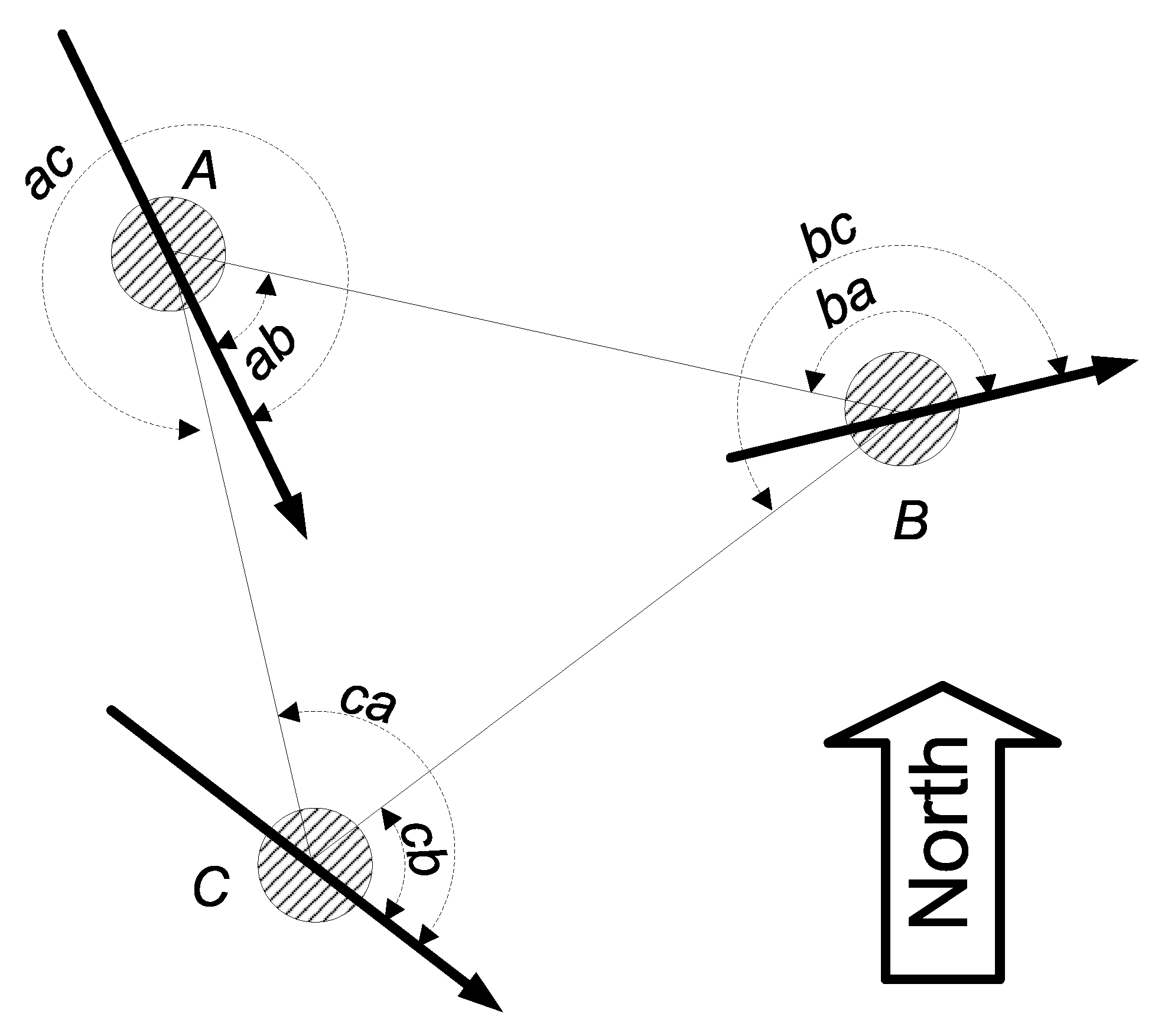
In many cases, practical situations require one to be aware of a sensor’s physical coordinates. Installing GPS receivers in every sensor is not always optimal from the cost-related and other perspectives. Typically, only a few nodes (seed nodes, landmarks, etc) of the network are equipped with GPS and know their physical location. The rest of the nodes can only communicate with other nodes and determine relative location characteristics such as distance, angles, etc. Various localization techniques are used to obtain location of all the sensors in the network. The following method assumes that the network consists of two types of nodes: usual and more capable nodes - which knows its position. Niculescu and Nath propose a method by which nodes in an ad hoc network collaborate in finding their position and orientation, assuming that a small part of the network has a position capability. Also, every node in the network has a capability to determine the angle of the arriving signal (AOA).

Each node in the network has one fixed main axis (which may not be the same for different nodes) and the node is able to measure all angles against this axis (Figure 1).

Figure 1. Nodes with AOA capability.

Figure 1. Nodes with AOA capability.

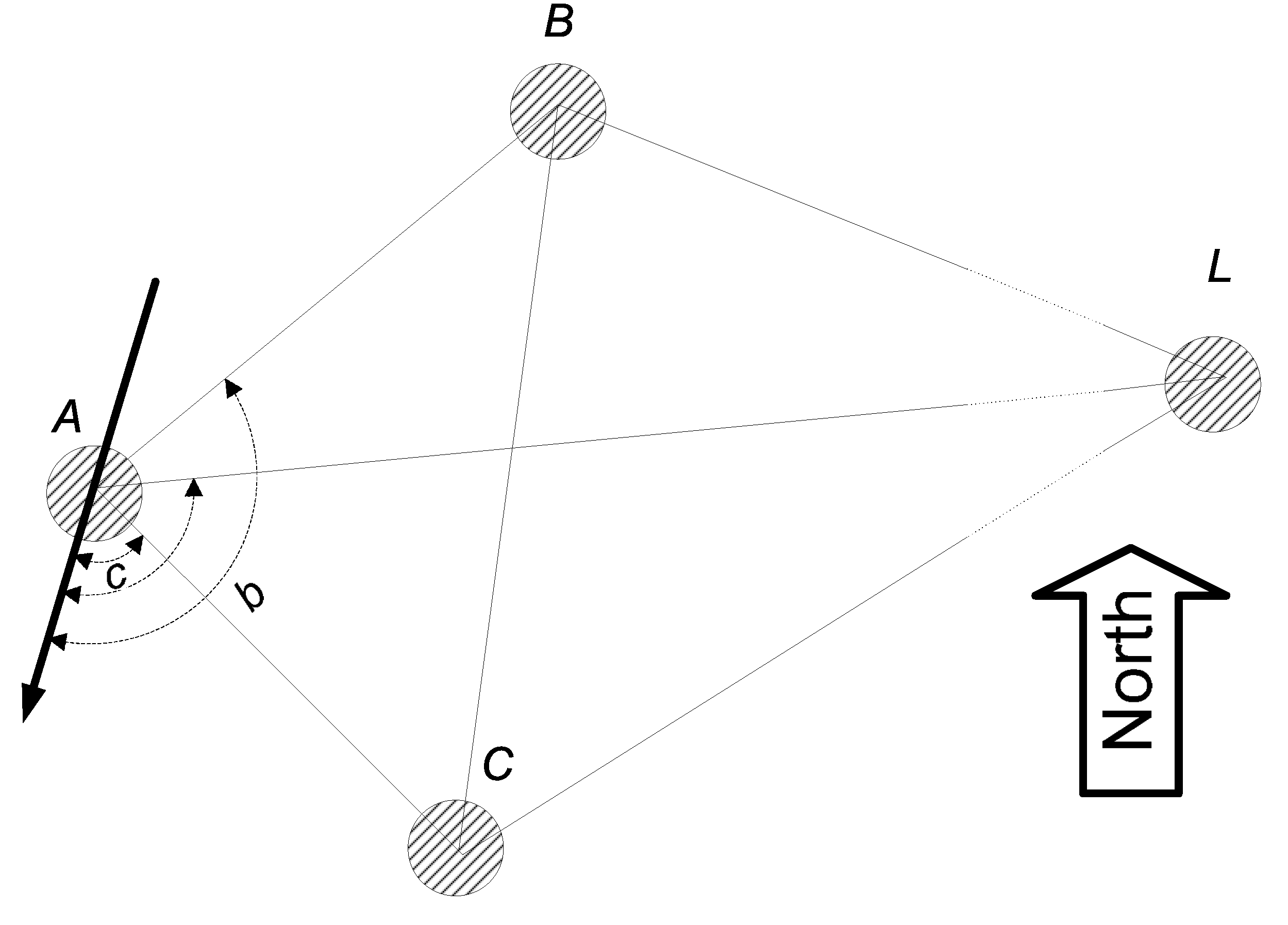
Every node in an ad hoc network can only communicate with its immediate neighbors within the radio range, and its neighbors may not always be landmarks, i.e., the nodes that know their position. Niculescu Nath propose in [17] a method to forward orientation in such way, that the nodes which are not in direct contact with landmarks can determine its orientation with respect to the landmarks. Orientation means bearing, radial, or both. Bearing is an angle measurement with respect to another object. A radial is the angle under which the object is seen from another point. The authors examine two algorithms: Distance Vector Bearing (DV-Bearing), which allows each node to get a bearing to landmark, and DV-Radial, which allows a node to get a bearing and radial to a landmark. The propagation in both algorithms works the following way: nodes adjacent to landmarks determine their bearing/radial directly from landmark and send to the network the information about their position. The method of computing node’s bearing and radial at each step is shown in Figure 2.

DV-Bearing algorithm works the following way. Nodes A, B, and C are neighbors and they can communicate with each other. Suppose that the node A needs to find its bearing to node L, which is not within radio range of node A but within radio range of nodes B and C. Since A, B, and C can locate each other than the node A can determine all the angles in triangles $ABC$ and $BCL$. But that would allow to calculate the angle $LAC$ and consequently the bearing of A to L, which is equal to $c+LAC$. Once node A knows three bearings to landmarks, which are not at the same line, then it can calculate its own location by triangulation.

The DV-Radial algorithm works the same way but with only one difference that node A needs to know not only bearings of nodes B and C to node L, but also the radials of B and C from L. The knowledge of radials improves accuracy of the algorithm. When all angles are measured against the same direction (for example, when compass is available) then these two methods become identical.

Figure 2. Node A computes its bearing to L using information from B and C

Figure 2. Node A computes its bearing to L using information from B and C

2.2. Semidefinite Programming (SDP) for Sensor Network Localization

The section considers localization problem when information on distances for anchor nodes and unknown sensors nodes are given. Suppose we consider localization problem on the plane. We have m known points $a_k\in {IR}^2$, $k=1,...,m$ and n unknown nodes $x_j\in {IR}^2$, $j=1,...,n$. Let us consider three sets of node pairs $N_e$, $N_l$, $N_u$. For pairs in $N_e$ we know exact distances $d_{kj}$ between $a_k$ and $x_j$ and $\widehat{d_{ij}}$ between $x_i$ and $x_j$. $N_l$ is a set of pairs with known lower bounds ${\underline{r}}_{kj}$ and ${\underline{r}}_{ij}$. Finally, $N_u$ is a set of upper bounds ${\overline{r}}_{kj}$ and ${\overline{r}}_{ij}$. Naturally our goal is to minimize estimation error which immediately lead us to the following non-convex optimization problem

$$\begin{array}{c}\hfill min\sum _{(i,j)\in N_e,i<j}|\parallel x_i-x_j{\parallel }^2-{\widehat{d}}_{ij}^2|\\ \hfill +\sum _{(k,j)\in N_e}|\parallel a_k-x_j{\parallel }^2-d_{kj}^2|\\ \hfill +\sum _{(i,j)\in N_l,i<j}(\parallel x_i-x_j{{\parallel }^2-{\underline{r}}_{ij}^2)}_{-}\\ \hfill +\sum _{(k,j)\in N_l}(\parallel a_k-x_j{{\parallel }^2-{\underline{r}}_{kj}^2)}_{-}\\ \hfill +\sum _{(i,j)\in N_u,i<j}(\parallel x_i-x_j{{\parallel }^2-{\overline{r}}_{ij}^2)}_{+}\\ \hfill +\sum _{(k,j)\in N_u}(\parallel a_k-x_j{{\parallel }^2-{\overline{r}}_{kj}^2)}_{+},\end{array}$$

(1)

where ${(u)}_{-}$ and ${(u)}_{+}$ are defined as

$$\begin{array}{ccc}& & {(u)}_{-}=max\{0,-u\}\hfill \\ & & {(u)}_{+}=max\{0,u\}.\hfill \end{array}$$

The norm of vector x is defined as $\parallel x\parallel =\sqrt{x^{T}x}$. In [18,19] the authors study semidefinite relaxations of the problem.

The formulated problem can be rewritten by introducing matrix notation and slack variables as

$$\begin{array}{ccc}& & \begin{array}{c}\hfill min\sum _{(i,j)\in N_e,i<j}({\alpha }_{ij}^{+}+{\alpha }_{ij}^{-})+\sum _{(k,j)\in N_e,}({\alpha }_{kj}^{+}+{\alpha }_{kj}^{-})\\ \hfill +\sum _{(i,j)\in N_l,i<j}{\beta }_{ij}^{-}+\sum _{(k,j)\in N_l}{\beta }_{kj}^{-}\\ \hfill +\sum _{(i,j)\in N_u,i<j}{\beta }_{ij}^{+}+\sum _{(k,j)\in N_u}{\beta }_{ij}^{+}\end{array}\hfill \\ & & \mathrm{s}.\mathrm{t}.\hfill \\ & & s_{ij}^{T}Y{e}_{ij}-d_{ij}2={\alpha }_{ij}^{+}-{\alpha }_{ij}^{-},\forall i,j\in N_e,i<j,\hfill \\ & & {(a_k;e_j)}^T\left(\begin{array}{cc}I& X\\ X^T& Y\end{array}\right)(a_k;e_j)-{({\widehat{d}}_{kj})}^2={\alpha }_{kj}^{+}-{\alpha }_{kj}^{-},\hfill \\ & & \forall k,j\in N_e,\hfill \\ & & e_{ij}^{T}Y{e}_{ij}-{(d_{ij})}^2\ge -{\beta }_{ij}^{-},\forall i,j\in N_l,i<j\hfill \\ & & {(a_k;e_j)}^T\left(\begin{array}{cc}I& X\\ X^T& Y\end{array}\right)(a_k;e_j)-{({\underline{r}}_{kj})}^2\ge -{\beta }_{kj}^{-},\hfill \\ & & \forall k,j\in N_l,\hfill \\ & & e_{ij}^{T}Y{e}_{ij}-{(d_{ij})}^2\le {\beta }_{ij}^{-},\forall i,j\in N_l,i<j\hfill \\ & & {(a_k;e_j)}^T\left(\begin{array}{cc}I& X\\ X^T& Y\end{array}\right)(a_k;e_j)-{({\underline{r}}_{kj})}^2\le {\beta }_{kj}^{-},\hfill \\ & & \forall k,j\in N_l,\hfill \\ & & {\alpha }_{ij}^{+},{\alpha }_{ij}^{-},{\alpha }_{kj}^{+},{\alpha }_{kj}^{-},{\beta }_{ij}^{+},{\beta }_{ij}^{-},{\beta }_{kj}^{+},{\beta }_{kj}^{-}\le 0,\hfill \\ & & Y=X^{T}X.\hfill \end{array}$$

Here $X=[x_1,x_2,\dots ,x_n]$ is a $2\times n$ matrix. In order to cope with nonconvexity equality, $Y=X^{T}X$ is replaced with $Y⪰X^{T}X$ or equivalently

$$Z:=\left(\begin{array}{cc}I& X\\ X^T& I\end{array}\right)⪰0.$$

The last relation leads to a standard SDP formulation:

$$\begin{array}{ccc}& & \begin{array}{c}\hfill min\sum _{(i,j)\in N_e,i<j}({\alpha }_{ij}^{+}+{\alpha }_{ij}^{-})+\sum _{(k,j)\in N_e,}({\alpha }_{kj}^{+}+{\alpha }_{kj}^{-})\\ \hfill +\sum _{(i,j)\in N_l,i<j}{\beta }_{ij}^{-}+\sum _{(k,j)\in N_l}{\beta }_{kj}^{-}\\ \hfill +\sum _{(i,j)\in N_u,i<j}{\beta }_{ij}^{+}+\sum _{(k,j)\in N_u}{\beta }_{ij}^{+}\end{array}\hfill \\ & & \mathrm{s}.\mathrm{t}.\hfill \\ & & {(1;0;\mathbf{0})}^{T}Z(1;0;\mathbf{0})=1,\hfill \\ & & {(0;1;\mathbf{0})}^{T}Z(0;1;\mathbf{0})=1,\hfill \\ & & {(1;1;\mathbf{0})}^{T}Z(1;1;\mathbf{0})=2,\hfill \\ & & {(\mathbf{0};e_{ij})}^{T}Z(\mathbf{0};e_{ij})-{\alpha }_{ij}^{+}+{\alpha }_{ij}^{-}={({\widehat{d}}_{ij})}^2,\forall i,j\in N_e,i<j,\hfill \\ & & {(a_k;e_j)}^{T}Z(a_k;e_j)-{\alpha }_{kj}^{+}+{\alpha }_{kj}^{-}={({\widehat{d}}_{kj})}^2,\forall k,j\in N_e,\hfill \\ & & {(\mathbf{0};e_{ij})}^{T}Z(\mathbf{0};e_{ij})+\beta {-}_{ij}\ge {({\underline{r}}_{ij})}^2,\forall i,j\in N_l,i<j,\hfill \\ & & {(a_k;e_j)}^{T}Z(a_k{e}_j)+{\beta }_{kj}^{-}\ge {({\underline{r}}_{kj})}^2,\forall k,j\in N_l,\hfill \\ & & {(\mathbf{0};e_{ij})}^{T}Z(\mathbf{0};e_{ij})-\beta {+}_{ij}\le {({\overline{r}}_{ij})}^2,\forall i,j\in N_u,i<j,\hfill \\ & & {(a_k;e_j)}^{T}Z(a_k{e}_j)-{\beta }_{kj}^{+}\le {({\overline{r}}_{kj})}^2,\forall k,j\in N_u,\hfill \\ & & {\alpha }_{ij}^{+},{\alpha }_{ij}^{-},{\alpha }_{kj}^{+},{\alpha }_{kj}^{-},{\beta }_{ij}^{+},{\beta }_{ij}^{-},{\beta }_{kj}^{+},{\beta }_{kj}^{-}\le 0,\hfill \\ & & Z⪰0.\hfill \end{array}$$

Papers [18,19] provide a criterion of solution existence and uniqueness, as well as statistical interpretation of the formulation in case when distance values are random values with normally distributed measurement errors. The SDP problems are solved using interior point algorithms. The numerical experiments results demonstrate the efficiency of the proposed approach.

3. Sensor Scheduling

Surveillance is an important task that can be effectively performed by an intelligent network of sensors. For example, satellites can be equipped with cameras to monitor Earth surface for different events, such as forest fire, border crossing or enemy hostile activity. Another example is traffic monitoring at the roads and intersections. Many scientific publications have recently appeared in the literature due to increasing interest to the problem of finding optimal schedule for sensors [20,21,22,23,24,25]. Most common technological and budget constraint is a low number of sensors to monitor all the objects of interest simultaneously. Thus, finding the schedule that reduces potential loss of limited observations is a task of high importance. This section provides a review of recently developed optimization based methods for building optimal schedule of sensor surveillance.

3.1. Single Sensor Scheduling

The simplest case is to model one sensor that observes a group of sites at discrete time points. Some physical systems require virtually zero time for changing a site being observed. For example, the time of a camera refocusing, which is installed on a satellite, is negligibly small. This assumption leads to the model proposed by Yavuz and Jeffcoat in [26].

Assume that we need to observe n sites during T time periods. During every period a sensor is allowed to watch only at one of n sites. The scheduling decision can be modeled using binary variables $x_{i,t}$

$$x_{i,t}=\left\{\begin{array}{cc}\hfill 1,& \mathrm{if }i\mathrm{-th site is observed at time }t,\hfill \\ \hfill 0,& \mathrm{otherwise},\hfill \end{array}\right.$$

(2)

t is a discrete variable and $t=1,2,...,T$. If a site i is not observed for some period of time, it leads to the penalty that is proportional to the time of not observing this site. This penalty can be modeled using another group of decision variables. Let $y_{i,t}$ denotes the time of last visiting site i before time moment t. Let us note that variables $x_{i,t}$ completely determine values of $y_{i,t}$. Fixed penalty $a_i$ and variable penalty $b_{it}$ are associated with site i at time moment t. Thus, the penalty at time t associated with site i is

$$a_i(1-x_{i,t})+b_{i,t}(t-y_{i,t}).$$

(3)

[26] suggests minimizing maximum loss over all sites and time intervals. Thus the objective function is defined as ${max}_{i,t}\{a_i+b_{i,t}(t-y_{i,t})\}$. This objective function can be linearized and consequently the problem looks as following

$$\begin{array}{ccc}& & minC\hfill \end{array}$$

(4)

$$\begin{array}{ccc}\hfill \mathrm{s}.\mathrm{t}.& & C\ge a_i(1-x_{i,t})+b_{i,t}(t-y_{i,t}),\forall i=1,\dots ,n,\forall t=1,\dots ,T,\hfill \end{array}$$

(5)

$$\begin{array}{ccc}& & \sum _{i=1}^n{x}_{i,t}\le 1,\forall t=1,\dots ,T,\hfill \end{array}$$

(6)

$$\begin{array}{ccc}& & 0\le y_{i,t}-y_{i,t-1}\le t{x}_{i,t},\forall i=1,\dots ,n,\forall t=1,\dots ,T,\hfill \end{array}$$

(7)

$$\begin{array}{ccc}& & t{x}_{i,t}\le y_{i,t}\le t,\forall i=1,\dots ,n,\forall t=1,\dots ,T,\hfill \end{array}$$

(8)

$$\begin{array}{ccc}& & y_{i,0}=0,\forall i=1,\dots ,n,\hfill \end{array}$$

(9)

$$\begin{array}{ccc}& & x_{i,t}\in \{0,1\},\forall i=1,\dots ,n,\forall t=1,\dots ,T,\hfill \end{array}$$

(10)

$$\begin{array}{ccc}& & y_{i,t}\in IR,\forall i=1,\dots ,n,\forall t=0,\dots ,T.\hfill \end{array}$$

(11)

Constraints (6) ensure that the sensor visits only one site at a time. Constraints (7) -(8 ) set the dependence $y_{i,t}$ on $x_{i,t}$. That is $y_{i,t}$ is set to t if and only if the sensor is observing site i at time t otherwise $y_{i,t}=y_{i,t-1}$.

Single Sensor Scheduling problem is NP-hard [27] therefore various greedy heuristics have been proposed. The idea behind greedy algorithm is simple. At time $t=1$ we find the site with the smallest penalty then at next time period we find another site with the smallest penalty. This sequence is repeated for all T time intervals. Thus the complexity of suggested approach is $O(nT)$. Yavuz and Jeffcoat has also suggested the “look ahead” modification of greedy heuristic which takes more computational time but computational experiment demonstrate that the solution is improved compared to the initial simple greedy optimization.

3.2. Stochastic approach

The stochastic nature of scheduling surveillance reduces the predictability of sensors behavior and therefore plays an important role for military tasks. Here we assume that sites are chosen randomly based on probability $p_{ij}$ of transition from i-th to j-th site . Then sensor scheduling can be considered as a Markov chain stochastic process and characterized by steady state probabilities ${\pi }_i$.

The goal of stochastic approach is finding such steady state probabilities that minimize maximum loss. Let $r_i$ be the visit period of site i. Then the penalty of information loss at site i is $a_i+(r_i-1)b_{i,t}$ at time t. Let us consider a sufficiently small planning horizon with time-invariant site dynamics, this allows us to reduce $b_{i,t}$ to $b_i$ and denote this approach as static. Visiting site i for every $r_i>0$ periods is equal to spending ${\pi }_i=1/r_i$ of the sensor’s time at the site i. The optimal schedule is achieved when ${\sum }_i{\pi }_i=1$; i.e., all the available time is utilized. Also, sensor never stays at any site for two consecutive periods of time. Thus $r_i\ge 2$ (or ${\pi }_i\le 0.5$) should be satisfied for each site. Then the non-linear model for obtaining optimal stationary probabilities is formulated as

$$\begin{array}{ccc}& & min\underset{i}{max}\{a_i+\left(\frac{1}{{\pi }_i}-1\right)b_i\}\hfill \end{array}$$

(12)

$$\begin{array}{ccc}\hfill \mathrm{s}.\mathrm{t}.& & \sum _{i=1}^n{\pi }_i=1,\hfill \end{array}$$

(13)

$$\begin{array}{ccc}& & {\pi }_i\le 0.5,\forall i=1,\dots ,n\hfill \end{array}$$

(14)

$$\begin{array}{ccc}& & {\pi }_i\in R,\forall i=1,\dots ,n\hfill \end{array}$$

(15)

$$\begin{array}{c}\hfill \end{array}$$

(16)

A heuristic is proposed to solve this nonlinear continuous problem. Utilizing constraints (14), the authors define a lower bound on the objective function value with

$$C^L=\underset{i}{max}\{a_i+b_i\}.$$

Then, we set

$$C=\underset{i}{max}\{a_i+\left(\frac{1}{\pi }-1\right)b_i\}=C^L$$

and calculate

$$r_i=(C-a_i)/b_i+1$$

and

$${\pi }_i=1/r_i$$

for all i. Note that ${\pi }_i=0.5$ for the sites with $a_i+b_i=C$ and ${\pi }_i<0.5$ for the remaining constraints. If the determined probabilities add up to one then the optimal solution is found, and the procedure terminates. If the sum of probabilities is less than one, then one can shift some π-s up to make ${\sum }_i{\pi }_i=1$. In the case when ${\sum }_i{\pi }_i>1$ the found C is infeasible and we can apply iterative procedures (such as bisection) to find C such that ${\sum }_i{\pi }_i=1$.

The static approach minimizes average penalty that is determined by steady probabilities and, thus, does not address the cases of long lasting absence at a site. Taking into account the fact that some random outcomes may result in extremely long penalties it is reasonable to increase the probabilities of visiting the sites that were visited long time ago. On the other hand, the probability of observing the sites, which were recently visited, should be decreased. Recall that $y_{i,t}$ represents the last time when the site i was visited by the time t. The probability of visiting a site must depend on the difference $t-y_{i,t}$, thus it will increase probability of visiting overdue sites.

To create a preference for visiting site i at time t the following adjustment factors are proposed

$$q_{i,t}={\pi }_i·{\left(\frac{t-y_{i,t}}{r_i}\right)}^k$$

It is bigger than one for overdue sites and less than one for the sites that have been visited within their expected visiting periods. The parameter k is a user-defined parameter, which determines the weight of the adjustment factor. The probabilities of visiting each site at specific time point t are based on previous history and can be computed as $p_i=q_i/Q$, where $Q={\sum }_{i=1}^n{q}_i$.

Finally, a hybrid method was proposed based on a combination of greedy algorithm and the stochastic method, discussed above. The first step calculates the penalty of not visiting site i: $c_i=a_i+b_{i,t}(t-y_{i,t}).$ Next step calculates preference values to visit each site: $q_i={\left(\frac{c_i}{c_{max}}\right)}^k,$ where $c_{max}={max}_i\left\{c_i\right\}.$ And then the probabilities of visit are equal to: $p_i=q_i/Q$, where $Q={\sum }_{i=1}^n{q}_i$.

3.3. Multiple Sensors Scheduling Using Percentile Type Constraints

Boyko et al have proposed to reformulate problem (4) -(11) for the case of m sensors [28].

$$\begin{array}{ccc}& & min\underset{i,t}{max}\{a_i+b_{i,t}(t-y_{i,t})\}\hfill \end{array}$$

(17)

$$\begin{array}{ccc}\hfill \mathrm{s}.\mathrm{t}.& & \sum _{i=1}^n{x}_{i,t}\le m,\forall t=1,\dots ,T,\hfill \end{array}$$

(18)

$$\begin{array}{ccc}& & 0\le y_{i,t}-y_{i,t-1}\le t{x}_{i,t},\forall i=1,\dots ,n,\forall t=1,\dots ,T,\hfill \end{array}$$

(19)

$$\begin{array}{ccc}& & t{x}_{i,t}\le y_{i,t}\le t,\forall i=1,\dots ,n,\forall t=1,\dots ,T,\hfill \end{array}$$

(20)

$$\begin{array}{ccc}& & y_{i,0}=0,\forall i=1,\dots ,n,\hfill \end{array}$$

(21)

$$\begin{array}{ccc}& & x_{i,t}\in \{0,1\},\forall i=1,\dots ,n,\forall t=1,\dots ,T,\hfill \end{array}$$

(22)

$$\begin{array}{ccc}& & y_{i,t}\in IR,\forall i=1,\dots ,n,\forall t=0,\dots ,T.\hfill \end{array}$$

(23)

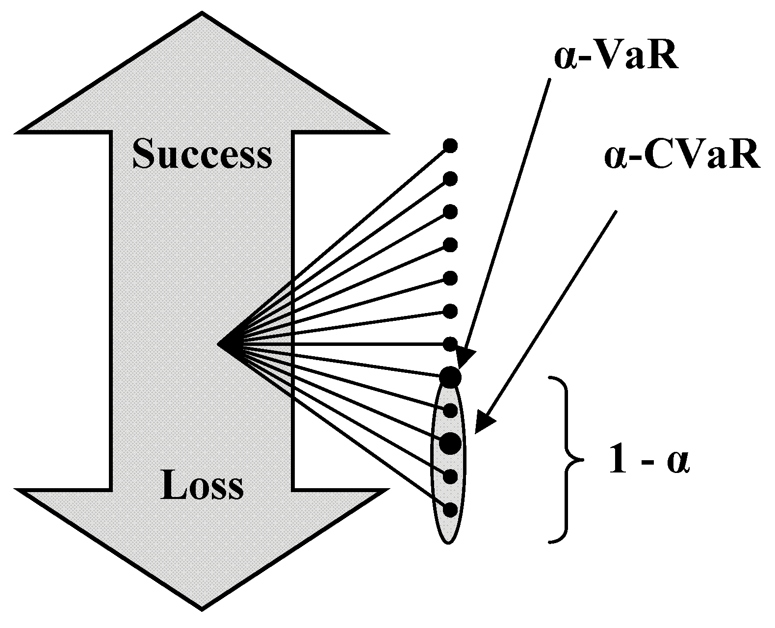
For every site i and every time point t we can calculate penalty associated with the last time a sensor visited this site $a_i+b_{i,t}(t-y_{i,t})$. Let us pick $(1-\alpha )$ % of worst cases among these $n\times T$ penalty values. Then, instead of minimizing maximum loss we can minimize the the average taken over this $(1-\alpha )$ % percent of worst penalty values. Despite the fact that this formulation is deterministic it is equivalent to computing $(1-\alpha )$ Conditional Value-at Risk (CVaR) for a set of random outcomes having equal probabilities $p_{i,t}=\frac{1}{nT}$.

CVaR [29,30] is closely related to a well-known quantitative risk measure referred to as Value-at-Risk (VaR). By definition with respect to a specified probability level $(1-\alpha )$ (in many applications the value of $(1-\alpha )$ is set rather high, e.g. 95%), the α-VaR is the lowest amount ζ such that with probability $(1-\alpha )$, the loss will not exceed ζ, whereas for continuous distributin the α-CVaR is the conditional expectation of losses above that amount ζ. As it can be seen, CVaR is a more conservative risk measure than VaR, which means that minimizing or restricting CVaR in optimization problems provides more robust solutions with respect to the risk of high losses (see figure 3).

Figure 3. Graphical representation of VaR and CVaR.

Figure 3. Graphical representation of VaR and CVaR.

The reader can find the formal definition of CVaR for various distribution cases in [29,30]. Rockafellar and Uryasev [31,32] showed that minimizing CVaR-type objective function of linear argument can be reduced to LP. In the sensors scheduling problem the loss function is introduced as

$$L(x,y,i,t)=a_i+b_{i,t}(t-y_{i,t}).$$

(24)

Thus the initial multiple sensors scheduling problem can be considered as the CVaR-based formulation

$$\begin{array}{ccc}& & \underset{x,y}{min}{\mathrm{CVaR}}_{\alpha }\left[L(x,y,i,t))\right]\hfill \end{array}$$

(25)

$$\begin{array}{ccc}& & \mathrm{s}.\mathrm{t}.\hspace{1em}\hspace{1em}\hspace{1em}\hspace{1em}\hspace{1em}\hspace{1em}\hspace{1em} \hfill \end{array}$$

$$\begin{array}{ccc}& & \mathrm{constraints }(18)-(23),\hfill \end{array}$$

$$\begin{array}{ccc}& & \zeta \in IR.\hspace{1em}\hspace{1em}\hspace{1em}\hspace{1em}\hspace{1em}\hspace{1em} \hfill \end{array}$$

(26)

Even though the parameters i and t of the loss function (24) are deterministic by nature, the stochastic framework was applied to this model in order to compute a percentile-type measure.

The parameters that quantify fixed and variable information losses are in many cases uncertain by nature. The following mathematical programming formulations allow quantifying and restricting the risks of worst-case losses associated with the aforementioned uncertain parameters. It is made by utilizing quantitative risk measures that allow one to control the robustness of the optimal solutions. Assuming that $a_i$ and $b_{i,t}$ are random values we can formulate stochastic program utilizing the notion of CVaR.

$$\begin{array}{c}\underset{x,y,\zeta }{\min }{\mathrm{CVaR}}_{\alpha }{a}_i^s(1-x_{i,t})+b_{i,t}^s(t-y_{i,t})\hfill \\ \mathrm{s}.\mathrm{t}.\hfill \\ \mathrm{constraints }(18)-(23).\hfill \end{array}$$

(27)

Here we use S scenarios ($a_i^s$ and $b_{i,t}^s$, $s=1,\dots ,S$) sampled from the distribution of penalty coefficients.

The mixed integer linear formulation was solved by ILOG CPLEX. The problems were also reformulated in terms of cardinality constraints and solved by AOrDa Portfolio Safeguard software package. Both solver find a good quality approximate solutions for large size problems.

4. Communication Network Interdiction

An important issue in military applications is to neutralize the communication in the sensors network of the enemy. This problem is known as jamming or eavesdropping a wireless communication network. This section introduces optimization formulations that allow to place jamming devices delivering maximal harm to the adverse sensors network. We start from a deterministic case when node locations are known.

The goal of jamming is to find a set of locations for placing jamming devices that suppresses the functionality of the network. Assume that n jamming devices are used to jam m communicating sensors. The assumption is made that the sensors and jammers can be located on a fixed set of locations V. The jamming effectiveness of device j is calculated as

$$d:(V\times V)\mapsto IR,$$

where d is a decreasing function of the distance from the jamming device to the node being jammed.

The cumulative level of jamming energy received at node i is defined as

$$Q_i:=\sum _{j=1}^n{d}_{ij},$$

where n is the number of jamming devices. Then, jamming problem can be formulated as the minimization of the number of jamming devices placed, subject to a set of covering constraints:

$$\begin{array}{ccc}& & \min n\hfill \\ & & \mathrm{s}.\mathrm{t}.Q_i\ge C_i,i=1,2,\dots ,m.\hfill \end{array}$$

Seeking the optimal placement coordinates $(x_j,y_j),j=1,2,\dots ,n$ for jamming devices given the coordinates $(X_i,Y_i),i=1,2,\dots ,m$ leads to non-convex formulations for most functions d. Thus, integer programming models for the problem are proposed.

A fixed set $\mathcal{N}=\{1,2,\dots ,n\}$ of possible locations for the jamming devices and the set of communication nodes are introduced by Commander et al in [33]. Define the decision variable $x_j$ as

$$x_j=\left\{\begin{array}{c}1,\mathrm{ if a jamming device is installed at location }j,\hfill \\ 0,\mathrm{ otherwise}.\hfill \end{array}\right.$$

(28)

Then we have the optimal network covering formulation given as

$$\begin{array}{ccc}& & min\sum _{j=1}^n{c}_j{x}_j\hfill \end{array}$$

(29)

$$\begin{array}{ccc}& & \mathrm{s}.\mathrm{t}.\hfill \end{array}$$

(30)

$$\begin{array}{ccc}& & \sum _{j=1}^n{d}_{ij}{x}_j\ge C_i,i=1,2,\dots ,m,\hfill \end{array}$$

(31)

$$\begin{array}{ccc}& & x_j\in \{0,1\},j=1,2,\dots ,n,\hfill \end{array}$$

(32)

Here the objective is to minimize the cost of jamming devices used while achieving some minimum level of coverage at each node. If $c_j=1$ then the number of jammers is minimized.

If the goal is to suppress sensors communications we can minimize jamming cost with respect to the required level of connectivity index. Communication between nodes i and j is assumed to be destroyed if at least one of the nodes is jammed. Further, let $y_{ij}:=1$ if there exists a path from node i to node j in the jammed network and let $z_i=1$ be an indicator that i-th node is jammed. This can be formulated as

$$\begin{array}{ccc}& & min\sum _{j=1}^n{c}_j{x}_j\hfill \end{array}$$

(33)

$$\begin{array}{ccc}& & \mathrm{s}.\mathrm{t}.\hfill \end{array}$$

$$\begin{array}{ccc}& & \sum _{\begin{array}{c}j=1\\ j\ne i\end{array}}^m{y}_{ij}\le L,\forall i\in \mathcal{M},\hfill \end{array}$$

(34)

$$\begin{array}{ccc}& & M(1-z_i)>S_i-C_i\ge -M{z}_i,\forall i\in \mathcal{M},\hfill \end{array}$$

(35)

$$\begin{array}{ccc}& & y_{ij}\mathrm{ is consistent with the network and }{z}_i\hfill \end{array}$$

(36)

$$\begin{array}{ccc}& & x_j\in \{0,1\},\forall j\in \mathcal{N},\hfill \end{array}$$

(37)

$$\begin{array}{ccc}& & z_i\in \{0,1\},\forall i\in \mathcal{M},\hfill \end{array}$$

(38)

$$\begin{array}{ccc}& & y_{ij}\in \{0,1\},\forall i,j\in \mathcal{M},\hfill \end{array}$$

(39)

where $S_i:={\sum }_{j=1}^n{d}_{ij}{x}_j$ denote the cumulative level of jamming at node i, $M\in IR$ is some large constant. This problem can be formulated as a mixed integer linear problem and justification is provided in [33].

Finally, Commander et al provide percentile-based formulation for deterministic jamming problems. Suppose it is determined that jamming some fraction $\alpha \in (0,1)$ of the nodes is sufficient for effectively dismantling the network. This can be accomplished by the inclusion of α-VaR constraints in the original model. Let $y:\mathcal{M}\mapsto \{0,1\}$ be an indicator whether node i is jammed ($y_i=1$).

Then to find the minimum number of jamming devices that will allow covering $\alpha ·100\%$ of the network nodes with prescribed levels of jamming $C_i$, we must solve the following integer program

$$\begin{array}{ccc}& & min\sum _{j=1}^n{c}_j{x}_j\hfill \end{array}$$

(40)

$$\begin{array}{ccc}& & \mathrm{s}.\mathrm{t}.\hfill \end{array}$$

$$\begin{array}{ccc}& & \sum _{i=1}^m{y}_i\ge \alpha m,\hfill \end{array}$$

(41)

$$\begin{array}{ccc}& & \sum _{j=1}^n{d}_{ij}{x}_j\ge C_i{y}_i,i=1,2,\dots ,m,\hfill \end{array}$$

(42)

$$\begin{array}{ccc}& & x_j\in \{0,1\},j=1,2,\dots ,n,\hfill \end{array}$$

(43)

$$\begin{array}{ccc}& & y_i\in \{0,1\},i=1,2,\dots ,m.\hfill \end{array}$$

(44)

The α-CVaR optimization model for network covering can be formulated as a mixed integer linear program using a standard linearization framework:

$$\begin{array}{ccc}& & min\sum _{j=1}^n{c}_j{x}_j\hfill \end{array}$$

(45)

$$\begin{array}{ccc}& & \mathrm{s}.\mathrm{t}.\hfill \end{array}$$

$$\begin{array}{ccc}& & \zeta +\frac{1}{(1-\alpha )m}\sum _{i=1}^{m}max\left\{C_{min}-\sum _{j=1}^n{x}_j{d}_{ij}-\zeta ,0\right\}\le 0,\hfill \end{array}$$

(46)

$$\begin{array}{ccc}& & \zeta \in \mathbb{R},\hfill \end{array}$$

(47)

$$\begin{array}{ccc}& & x_j\in \{0,1\}.\hfill \end{array}$$

(48)

The VaR and CVaR models can also be written for connectivity suppression models in the similar fashion. We refer the reader to [33] for details.

The deterministic formulations of the wireless network jamming problem are extended in [34] to tackle the stochastic jamming problem formulations using percentile type constraints. These formulations consider the case when the exact topology of the network to be jammed is not known, but we know the distribution of network parameters.

Since the exact locations of the network nodes are unknown, it is assumed that a set of intelligence data has been collected and from that a set $\mathcal{S}$ of the most likely scenarios have been compiled. Scenario $s\in \mathcal{S}$ contains both the node locations $\{({\xi }_1^s,{\eta }_1^s),({\xi }_2^s,{\eta }_2^s),\dots ,({\xi }_m^s,{\eta }_m^s)\}$ and the set of jamming thresholds $\{C_1^s,C_2^s,\dots ,C_m^s\}$. For each scenario $s\in \mathcal{S}$, the set ${\mathcal{M}}_s=\{1,2,\dots ,m_s\}$ needs to be jammed. Taking into account all the scenarios we can write a mathematical program for node covering problem:

$$\begin{array}{ccc}& & min\sum _{k=1}^n{c}_k{x}_k,\hfill \end{array}$$

(49)

$$\begin{array}{ccc}& & \mathrm{s}.\mathrm{t}.\hfill \end{array}$$

$$\begin{array}{ccc}& & \sum _{k=1}^n{d}_{ik}^s{x}_k\ge C_i^s,i=1,2,\dots ,m_s,s=1,2,\dots ,S,\hfill \end{array}$$

(50)

$$\begin{array}{ccc}& & x_k\in \{0,1\},k=1,2,\dots ,n,\hfill \end{array}$$

(51)

It is unlikely to find the solution that can provide effective jamming strategy for all scenarios. Therefore, the notion of percentile-based risk measures can be utilized to develop formulations of the robust jamming problems incorporating these risk constraints. The robust node covering problem with Value-at-Risk constraints can be formulated as

$$\begin{array}{ccc}& & min\sum _{k=1}^n{c}_k{x}_k,\hfill \end{array}$$

(52)

$$\begin{array}{ccc}& & \mathrm{s}.\mathrm{t}.\hfill \end{array}$$

$$\begin{array}{ccc}& & \sum _{k=1}^n{d}_{ik}^s{x}_k\ge C_i^s{\rho }_i^s,\forall s\in \mathcal{S},\forall i\in {\mathcal{M}}_s,\hfill \end{array}$$

(53)

$$\begin{array}{ccc}& & \sum _{i=1}^{m_s}{\rho }_i^s\ge \alpha m_s,\forall s\in \mathcal{S},\hfill \end{array}$$

(54)

$$\begin{array}{ccc}& & x_k\in \{0,1\},\forall k\in \mathcal{N},\hfill \end{array}$$

(55)

$$\begin{array}{ccc}& & {\rho }_i^s\in \{0,1\},\forall s\in \mathcal{S},\forall i\in {\mathcal{M}}_s,\hfill \end{array}$$

(56)

The loss function can be considered as the difference between the energy required to jam network node i, namely $C_i^s$, and the cumulative amount of energy received at node i due to x over each scenario. With this the robust node covering problem with CVaR constraints is formulated as follows.

$$\begin{array}{ccc}& & min\sum _{k=1}^n{c}_k{x}_k,\hfill \end{array}$$

(57)

$$\begin{array}{ccc}& & \mathrm{s}.\mathrm{t}.\hfill \end{array}$$

$$\begin{array}{ccc}& & {\zeta }^s+\frac{1}{(1-\alpha )m_s}\hfill \end{array}$$

(58)

$$\begin{array}{ccc}& & \sum _{i=1}^{m_s}max\left\{C_{min}^s-\sum _{k=1}^n{d}_{ik}^s{x}_k-{\zeta }^s,0\right\}\le 0,\forall s\in \mathcal{S},\hfill \end{array}$$

(59)

$$\begin{array}{ccc}& & x_k\in \{0,1\},\forall k\in \mathcal{N},\hfill \end{array}$$

(60)

$$\begin{array}{ccc}& & {\zeta }^s\in \mathbb{R},\forall s\in \mathcal{S}.\hfill \end{array}$$

(61)

The CVaR constraint (59) implies that for the $(1-\alpha )·100\%$ of the worst (least) covered nodes, the average value of $f(x)$ is less than or equal to 0.

Numerical experiments demonstrate that problems of moderate size can be solved by ILOG CPLEX. Finding effective heuristics and approximations for sensors network jamming problems of large dimensions is an interesting and important research direction.

5. Conclusion

In this paper, we presented a brief outline of problems and challenges arising in the important and exciting area of mathematical programming techniques for sensor network applications. Clearly, the research in this area is far from complete, and a lot of extensions and generalizations of the presented models can be developed. Overall, the main challenges arising in this area are associated with efficiently incorporating the uncertainties in the mathematical programming formulations and dealing with the computational intractability of the corresponding stochastic and robust optimization problems. However, there are promising developments in this field, including computationally efficient heuristic algorithms and software packages for solving these problems. Therefore, the area of sensor networks and mathematical programming techniques associated with it has a clear potential from both theoretical and practical perspectives.