Article

Mixed Variational Formulations for Micro-cracked Continua in the Multifield Framework

Department of Structural Mechanics, University of Pavia, via Ferrata 1, Pavia, Italy
*
Author to whom correspondence should be addressed.
Algorithms 2009, 2(1), 606-622; https://doi.org/10.3390/a2010606
Submission received: 9 March 2009 / Accepted: 24 March 2009 / Published: 27 March 2009
(This article belongs to the Special Issue Numerical Simulation of Discontinuities in Mechanics)

Abstract

:
Within the framework of multifield continua, we move from the model of elastic microcracked body introduced in (Mariano, P.M. and Stazi, F.L., Strain localization in elastic microcracked bodies, Comp. Methods Appl. Mech. Engrg. 2001, 190, 5657–5677) and propose a few novel variational formulations of mixed type along with relevant mixed FEM discretizations. To this goal, suitably extended Hellinger-Reissner principles of primal and dual type are derived. A few numerical studies are presented that include an investigation on the interaction between a single cohesive macrocrack and diffuse microcracks (Mariano, P.M. and Stazi, F.L., Strain localization due to crack–microcrack interactions: X–FEM for a multifield approach, Comp. Methods Appl. Mech. Engrg. 2004, 193, 5035–5062).

1. Introduction and modeling

1.1. Introductory remarks

A wide class of theoretical and technological problems are related to the mechanical description and the practical use of bodies endowed with a large number of microcracks scattered throughout the volume. Reference is made to [7] for a detailed review of these problems. When microcracks are dilute in the sense that the interactions between them are not prominent and also the microcrack distribution is approximately periodic, standard homogenization procedures can be advantageously applied to describe the influence of the microcracks on the gross behavior, see e.g. [14]. Conversely, when microcracks are dense in a way that the interactions between them are prominent and also their distribution is not homogeneous, non–negligible gradients are involved and standard homogenization procedure cannot be used in standard way. Precisely the microcracked body has to be considered strictly as a complex body and its description falls naturally within the setting of multi–field theories representing complex bodies. Here we pay attention to bodies with a dense population of microcracks scattered throughout a "soft" matrix of material. In particular we try to describe the influence on the gross behavior of the deformation of microcracks, considered both as sharp defects (pieces of planes not interpenetrated by interatomic bonds) and/or as elliptic voids with one dimension very small with respect to the others. The following treatment is restricted to elasticity, since any irreversible growth of microcracks (damage evolution) is not accounted for. The basic aim of the paper is to represent in some way sub–structural interactions due to microcrack changes in a scattered sense. Since we consider dense populations of microcracks we follow here a multi–field model of microcracked bodies that has been already formulated in a series of papers (see [9] and references therein). This approach seems to predict verifiable non–usual phenomena, namely strain localization that straightforwardly arise from the adopted model notwithstanding the linear elastic regime. The model takes into account two vectorial components of a global displacement field, namely macro–displacements and micro–displacements. The constitutive relationships described in Section 1.2. allow to link their gradients to the relevant macro and micro stress fields.
The numerical investigations discussed in [9] and [10] refer to displacement–based finite element methods that adopt post–processing techniques to derive the stress fields. The present paper proposes instead ad hoc mixed formulations that interpolate independently stresses and displacements. The mixed scheme is adopted both at the macro and micro level, thus providing a numerical framework that allows a direct discretization of displacements and stresses that arise at the two scales. Suitably extended Hellinger-Reissner principles of primal and dual type are derived to this purpose in Section 2.. Two different solutions are herein discussed. The first adopts displacements as main variables, while stresses play the role of Lagrangian multipliers. The second, the so–called "truly–mixed" formulation [2], implements a dual approach where the stresses are main unknowns of the elastic problem. Peculiar attention is paid to the interactions between a macrocrack and diffuse microcracks. Details of the implementation are discussed in Section 2.3., while two numerical examples are illustrated in Section 3.. The first is devoted to assess the capabilities of the proposed method to predict localization phenomena not only in the micro displacement field, as already shown in [9], but also in the micro stress one. Afterwards, the second example allows to discuss the effects of the presence of a single macrocrack within the diffuse microcracks peculiar to the adopted multifield model. Particular attention is devoted in this case to the convergence features of the proposed method. Section 4. concludes the paper introducing the ongoing developments.

1.2. The constitutive model

Concerning the constitutive model, the purpose of this section is to present the basic equations governing micro–fractured media modeled within the framework of multifield continua. Reference is made to [8] for an exhaustive treatment on this subject and to [9] for the micro–fractured model investigated herein. For simplicity sake, we adopt the hypothesis of small displacements and strains.
Figure 1. The lattice model.
Algorithms 02 00606 g001
Within this assumption, the macro and micro equilibrium equations may be respectively written as
div ̲ T ̲ ̲ + b ̲ = 0 ̲ , z ̲ + div ̲ S ̲ ̲ = 0 ̲ ,
where T ̲ ̲ and S ̲ ̲ are the (usual) Cauchy and micro stress tensors, b ̲ is the load per unit area and z ̲ is the self-force, the static dual of the micro-displacement vector d ̲ . Coming to the compatibility equations, an additive decomposition of the displacement field is introduced as
U ̲ = u ̲ + d ̲ ,
along with the linear kinematics hypothesis
ε ̲ ̲ u ( u ̲ ) = 1 2 ( ̲ ̲ u ̲ + ̲ ̲ u ̲ T ) ̲ ̲ s u ̲ ε ̲ ̲ d ( d ̲ ) = 1 2 ( ̲ ̲ d ̲ + ̲ ̲ d ̲ T ) ̲ ̲ s d ̲ .
The constitutive law of the proposed model should provide relations between macro-stresses T ̲ ̲ and macro-strains ̲ ̲ s u ̲ , micro-stresses S ̲ ̲ and micro-strains ̲ ̲ s d ̲ and cross–terms between macro and micro static and kinematic quantities. Furthermore, the self-force z ̲ is to be related to the micro displacement vector d ̲ . The procedure for the derivation of such constitutive relationships cannot take much advantage of experimental tests due to the microscopic nature of the involved quantities. Therefore, a mathematical procedure has been presented in [9] that moves from the lattice model shown in Figure 1. By equating the internal power of the lattice model to the one of an equivalent multifield continuum, one can show that the following constitutive equations are arrived at
T ̲ ̲ = A ̲ ̲ u ̲ B ̲ ̲ d ̲ S ̲ ̲ = B ̲ ̲ u ̲ + G ̲ ̲ d ̲ , z ̲ = C d ̲
where
A = W M 2 R V E m 2 + 1 / 2 0 0 1 / 2 1 / 2 1 / 2 0 1 / 2 0 2 + 1 / 2 + 1 2 M 2 H R V E M R V E m 1 0 0 1 1 1 0 1 0 1 ,
G = 1 2 Q m 2 R V E m 1 0 0 1 1 1 0 1 0 1 + 1 2 m 2 H R V E M R V E m 1 0 0 1 1 1 0 1 0 1 ,
B = 1 2 m 2 M 2 H R V E M R V E m 1 0 0 1 1 1 0 1 0 1 , C = 2 Q R V E m 1 0 0 1 .
The phisical parameters entering the equations above are defined as follows (see also Figure 1 for the definitions of the caracteristic lengths M , m and C ):
t= specimen thickness
R V E M = material reference volume element = M 2 t
R V E m = micro-fracture reference volume element = m 2 t
E= Young modulus of the bonds between macro-spheres
E * = Young modulus of the bonds between macro-spheres and micro-holes
W =  E A / M = macro-lattice stiffness
Q =  E A / ( π c ) = mean stiffness of the ellipsoidal micro-holes
H =  2 E A / [ 2 ( m M ) ] = stiffness of the bonds between macro and meso lattices
A ^ = cross section of rods between adjacent micro-cracks.
In view of the derivation of mixed variational principles of Hellinger–Reissner type, generalized to cope with multifield problems, the formal inverse of the constitutive law (4) is written as
̲ ̲ s u ̲ = E T ̲ ̲ + H S ̲ ̲ ̲ ̲ s d ̲ = H T ̲ ̲ + M S ̲ ̲ z ̲ = C d ̲ ,
where
E H H M
is the inverse of the constitutive matrix derived from its direct form, i.e.
A B B G .

2. Mixed variational formulations

This section is devoted to the derivation of the two Hellinger–Reissner formulations for the herein considered multifield framework. The first formulation, further addressed as Primal Hellinger–Reissner formulation, has regular displacements as main variables, while discontinuous stresses play the role of Lagrangian multipliers. The Dual Hellinger–Reissner formulation conversely adopts regular stresses as principal unknowns, while discontinuous approximations may be used for the displacements. Reference is made to [2] for further details on the formulations within the classical Cauchy continuum and to [4] for an implementation of the two above mixed formulations.
Peculiar attention will be paid in the following sections to the inclusion of a macrocrack within the microcracked model. Discussions on the adoption of cohesive models within a mixed frameworks may be also found in [3].

2.1. Primal Hellinger–Reissner formulation

To derive the first block of equations one may use the compatibility (3) and constitutive equations (5) 1 , 2 to get rid of macro and micro strain fields, and subsequently testing the resulting two equations with a macro–stress field τ ̲ ̲ and a micro–stress field σ ̲ ̲ . The second block of equations may be derived testing the two equilibrium equations (1) with virtual macro and micro displacement fields, say v ̲ and e ̲ . The achieved formulation reads: Find ( T ̲ ̲ , S ̲ ̲ , u ̲ , d ̲ ) L 2 ( Ω ) × L 2 ( Ω ) × H 1 ( Ω ) × H 1 ( Ω ) such that:
Ω E ̲ ̲ ̲ ̲ T ̲ ̲ : τ ̲ ̲ + Ω H ̲ ̲ ̲ ̲ S ̲ ̲ : τ ̲ ̲ Ω ̲ ̲ s u ̲ : τ ̲ ̲ = 0 Ω H ̲ ̲ ̲ ̲ T ̲ ̲ : σ ̲ ̲ + Ω M ̲ ̲ ̲ ̲ S ̲ ̲ : σ ̲ ̲ Ω ̲ ̲ s d ̲ : σ ̲ ̲ = 0 Ω T ̲ ̲ : s v ̲ = F u Ω S ̲ ̲ : ̲ ̲ s e ̲ Ω C ̲ ̲ d ̲ · e ̲ = F d
( τ ̲ ̲ , σ ̲ ̲ , v ̲ , e ̲ ) L 2 ( Ω ) × L 2 ( Ω ) × H 1 ( Ω ) × H 1 ( Ω ) , where
F u = Ω b ̲ · v ̲ Γ ( T ̲ ̲ · n ̲ ) · v ̲ F d = Γ ( S ̲ ̲ · n ̲ ) · v ̲ ,
that fits the usual mixed–method algebraic format, i.e.
A T T A T S B T u 0 A S T A S S 0 B S d B u T 0 0 0 0 B d S 0 C d d T S u d = 0 0 F u F d
Referring to the finite element discretization, one can use the standard P 1 P 0 triangular approximation that has been actually implemented in the numerical examples to follow. When a macroscopic fracture is to be added to the model, functional spaces should be slightly modified to allow displacement discontinuities. Furthermore, stress flux continuity across the crack should be enforced by using suitable Lagrange multipliers.
Formally, by testing the macro–equilibrium equation (1) 1 and using Gauss–Green formula one gets:
Ω div ̲ T ̲ ̲ · v ̲ = Γ T ̲ ̲ · n ̲ · v ̲ Ω T ̲ ̲ : ̲ ̲ s v ̲ .
To deal with the inclusion of a macrocrack one may specialize the line integral on Γ in (8) along the two adjacent edges of the fracture Γ c , with normal n ̲ . One has therefore to introduce the displacement jump [[ v ̲ ]] that denotes the prescribed discontinuity along the crack. The continuous stress fluxes may be written as:
T ̲ ̲ · n ̲ = C ̲ ̲ 1 [[ u ̲ ]]
taking into account the constitutive parameter C ̲ ̲ that holds the cohesive law, i.e. the mechanical relationship that ties the vector of the displacement discontinuities to the vector of the stress–fluxes.
According to the above issues, the achieved primal mixed variational formulation for microcracked bodies that embed discrete macrocracks reads: Find ( T ̲ ̲ , S ̲ ̲ , u ̲ , d ̲ ) L 2 ( Ω ) × L 2 ( Ω ) × H 1 ( Ω ) × H 1 ( Ω ) such that:
Ω E ̲ ̲ ̲ ̲ T ̲ ̲ : τ ̲ ̲ + Ω H ̲ ̲ ̲ ̲ S ̲ ̲ : τ ̲ ̲ Ω ̲ ̲ s u ̲ : τ ̲ ̲ = 0 Ω H ̲ ̲ ̲ ̲ T ̲ ̲ : σ ̲ ̲ + Ω M ̲ ̲ ̲ ̲ S ̲ ̲ : σ ̲ ̲ Ω ̲ ̲ s d ̲ : σ ̲ ̲ = 0 Ω T ̲ ̲ : s v ̲ + Γ c C ̲ ̲ [ [ u ̲ ] ] · [ [ v ̲ ] ] = F u Ω S ̲ ̲ : ̲ ̲ s e ̲ Ω C ̲ ̲ d ̲ · e ̲ = F d
( τ ̲ ̲ , σ ̲ ̲ , v ̲ , e ̲ ) L 2 ( Ω ) × L 2 ( Ω ) × H 1 ( Ω ) × H 1 ( Ω ) .
It must be remarked that the primal mixed formulation is similar to a classical displacement–based approach in the sense that the continuity of the displacement field is required in both the case by the variational formulation. In practice, the displacement discontinuity that has to be introduced across an evolving crack has been modeled in Section 3. by doubling the nodes across the fracture.

2.2. Dual Hellinger–Reissner formulation

The alternative truly–mixed formulation may be recovered by applying Gauss–Green formula (8) to equation (6), in order to transfer regularity form the displacement fields to the stress ones. One straightforwardly gets: Find ( T ̲ ̲ , S ̲ ̲ , u ̲ , d ̲ ) H ( div ̲ ̲ , Ω ) × H ( div ̲ , Ω ) × L 2 ( Ω ) × L 2 ( Ω ) such that:
Ω E ̲ ̲ ̲ ̲ T ̲ ̲ : τ ̲ ̲ + Ω H ̲ ̲ ̲ ̲ S ̲ ̲ : τ ̲ ̲ + Ω u ̲ · div ̲ τ ̲ ̲ = F T Ω H ̲ ̲ ̲ ̲ T ̲ ̲ : σ ̲ ̲ + Ω M ̲ ̲ ̲ ̲ S ̲ ̲ : σ ̲ ̲ + Ω d ̲ · div ̲ σ ̲ ̲ = F S Ω div ̲ T ̲ ̲ · v ̲ = F u Ω div ̲ S ̲ ̲ · e ̲ Ω C ̲ ̲ d ̲ · e ̲ = 0
( τ ̲ ̲ , σ ̲ ̲ , v ̲ , e ̲ ) H ( div ̲ , Ω ) × H ( div ̲ , Ω ) × L 2 ( Ω ) × L 2 ( Ω ) , where
F T = Γ u ̲ · ( τ ̲ ̲ · n ̲ ) F S = Γ d ̲ · ( σ ̲ ̲ · n ̲ ) F u = Ω b ̲ · v ̲
As found in the previous section the above formulation may be written according to the usual mixed–method algebraic format of (7).
The finite element scheme however presents additional troubles with respect to the previous case, due to the well–known stability requirement that goes under the name of inf–sup condition [2]. Only a few discretizations pass this requirement providing full robustness even in the presence of incompressible materials. Among the others, reference is made to the composite triangle of Johnson and Mercier, [6].
An attractive feature of the introduced "truly–mixed" setting resides in the possibility of straightforwardly modeling cohesive macrocracks within the variational formulation. Looking at the functional spaces introduced in (11) one may easily notice that a discontinuity in the displacements naturally arises from the variational principle, while the required regularity on the stress fields simply consists in a continuity of the stress–fluxes. These two issues therefore allows to implement a cohesive macro–fracture that may be taken into account through the following modified formulation, i.e.: Find ( T ̲ ̲ , S ̲ ̲ , u ̲ , d ̲ ) H ( div ̲ ̲ , Ω ) × H ( div ̲ , Ω ) × L 2 ( Ω ) × L 2 ( Ω ) such that:
Ω E ̲ ̲ ̲ ̲ T ̲ ̲ : τ ̲ ̲ + Ω H ̲ ̲ ̲ ̲ S ̲ ̲ : τ ̲ ̲ + Ω u ̲ · div ̲ τ ̲ ̲ = F T Ω H ̲ ̲ ̲ ̲ T ̲ ̲ : σ ̲ ̲ + Ω M ̲ ̲ ̲ ̲ S ̲ ̲ : σ ̲ ̲ + Ω d ̲ · div ̲ σ ̲ ̲ = F S Ω div ̲ T ̲ ̲ · v ̲ + Γ c C ̲ ̲ [ [ u ̲ ] ] · [ [ v ̲ ] ] = F u Ω div ̲ S ̲ ̲ · e ̲ Ω C ̲ ̲ d ̲ · e ̲ = 0
( τ ̲ ̲ , σ ̲ ̲ , v ̲ , e ̲ ) H ( div ̲ , Ω ) × H ( div ̲ , Ω ) × L 2 ( Ω ) × L 2 ( Ω )

2.3. Implementation

From a computational point of view, the problem is mainly characterized, in comparison to a classical Cauchy problem, by the presence of twice as many discretization fields. In fact we discretize the macro stress and macro displacements fields typical of a plane problem and their corresponding micro quantities. This fact suggests to pay attention to the storage scheme of the final solving system, considering in particular the solution method to be profitably adopted. To speed up the code, the assembling procedure has been optimized by means of a parallelization introduced in the making of macro and corresponding micro stiffness matrixes. Such a method leads to have a final sparse structure that is composed by block matrixes which must be handled through specific solvers. A few algorithms are available in the literature for the solutions of indefinite linear systems of the type (7).
One may resort to solvers belonging to the Uzawa family and its inexact variants. These methods have an iterative nature and often require a clever and often cumbersome choice of the relevant parameters to achieve the expected convergence in a small number of iterations. For this reason the performed analysis resort to the the algorithm PARDISO [12,13] that was especially conceived for the solution of large indefinite linear systems.

3. Numerical studies

The following session has the aim of validating the previous theoretical framework through some relevant numerical investigations. The first Hellinger Reissner formulation is herein implemented in order to investigate the capabilities of the mixed setting to deal with multifield approaches.
The first example deals the benchmark problem originally presented in [9], that was especially conceived to show the arising of remarkable localizations in the displacement fields when adopting displacement–based techniques. The mixed formulation is tested on this example to capture not only the above localizations on displacements but also the ones that may affect micro stresses.
The second example deals with the interactions of a macrocrack with the considered microcracked continuum. The problem was firstly tackled in [10], according to a variation of the well–known displacement–based X-FEM procedure [11]. The same example is also used to show some results on the convergence features of the proposed mixed schemes.
It must be highlighted that both the examples exploit a peculiar feature of the mixed methods, i.e. the accuracy in the approximation of the stress field that mainly descends form its independent interpolation with respect to the displacement field.

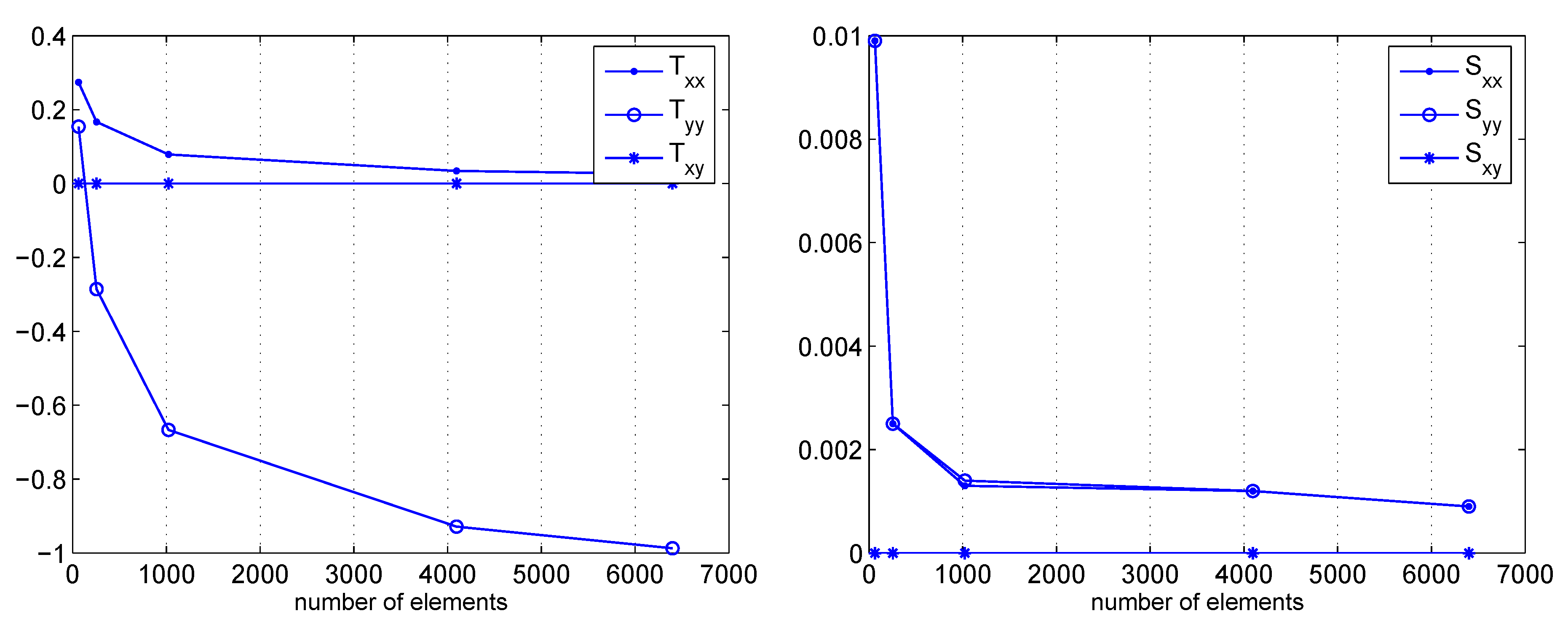
3.1. A clamped square lamina

Following [9], a square membrane is considered clamped at the left side and loaded at the mid–point on the right side. The physical quantities of the adopted model are specified in Table 1, while the geometry of the specimen is illustrated in Figure 2.
Concerning boundary conditions, both micro and macro displacements fields are constrained to zero translations at the left side of the domain. At the right side, the node in the middle, loaded by the force F, is also constrained by an imposed micro displacement equal to δ (see [9] for a discussion on this issue).
Table 1. Physical parameters.
m [ m m ] M [ m m ] δ [ m m ] E [ N / m m 2 ] A [ m m 2 ] A ^ [ m m 2 ] C m m χ
20010.1 10 5 10.314150
Figure 2. The loaded plane membrane.
Algorithms 02 00606 g002
Figure 3 and Figure 4 show the components of the macro and micro displacements in both the directions. The resulting global displacement field is plotted in Figure 5. The last figure clearly shows the capability of the model in capturing the strain localization of the two 45–degree oriented stripes that arise from the load application point. This behavior is exclusively due to the multifield nature of the model, since macro displacements plots are free from any localization phenomenon and exhibit the usual smoothness expected in the context of a classical Cauchy continuum. The strong localizations take place in the micro displacement components and have such a remarkable magnitude that they considerably affect the resulting (additive) global displacement field of Figure 5.
These results, concerning the displacement fields, are in perfect agreement with those achieved by the displacement–based method used in [9]. Additionally, the mixed method herein implemented allows for a straightforward prediction of the stress fields, since they are independently interpolated as variables of the multifield elastic problem. No post–processing technique is required in this case, thus providing the expected accuracy in the evaluation of all the unknowns involved in the problem.
Figure 6, Figure 7 and Figure 8 describe a similar behavior with respect to the one already discussed concerning the displacements. Macro stresses show in fact the smooth behavior peculiar to tensors of the Cauchy type. Micro stresses follow instead the localization already captured in the displacements plots with similar 45–degree oriented stripes that moves form the singularity point. In this case stress concentrations that have a similar magnitude with respect to the corresponding macro-quantities affect the three components of the micro–tensors in the region next to the load application zone.
It is also interesting to point out that the symmetry of micro stresses is not imposed by the rotation balance, as for the Cauchy macro tensor, but is herein recovered via the constitutive law, see Section 1.2..
Figure 3. Macro–displacements u x - Micro–displacements d x .
Algorithms 02 00606 g003
Figure 4. Macro–displacements u y - Micro–displacements d y .
Algorithms 02 00606 g004
Figure 5. Global displacements u x + d x - u y + d y .
Algorithms 02 00606 g005
Figure 6. Macro–stress T x x - Micro–stress S x x .
Algorithms 02 00606 g006
Figure 7. Macro–stress T y y - Micro–stress S y y .
Algorithms 02 00606 g007
Figure 8. Macro–stress T x y - Micro–stress S x y .
Algorithms 02 00606 g008

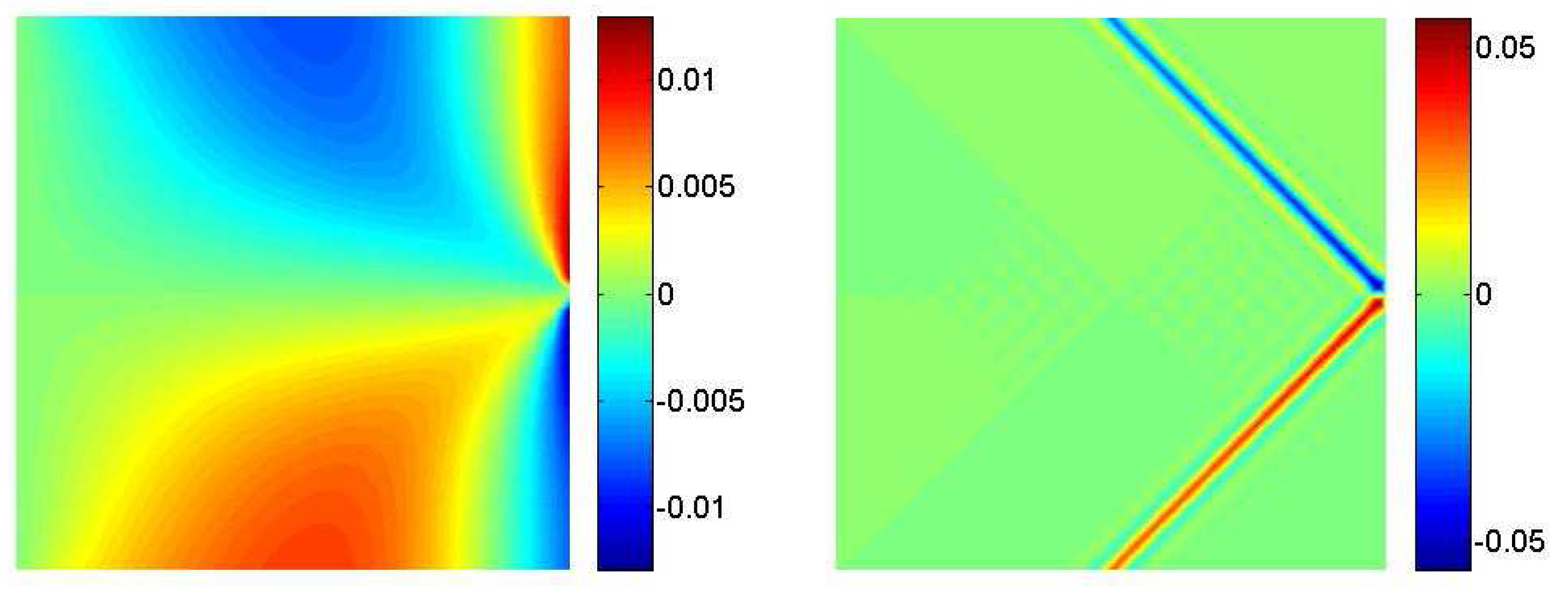
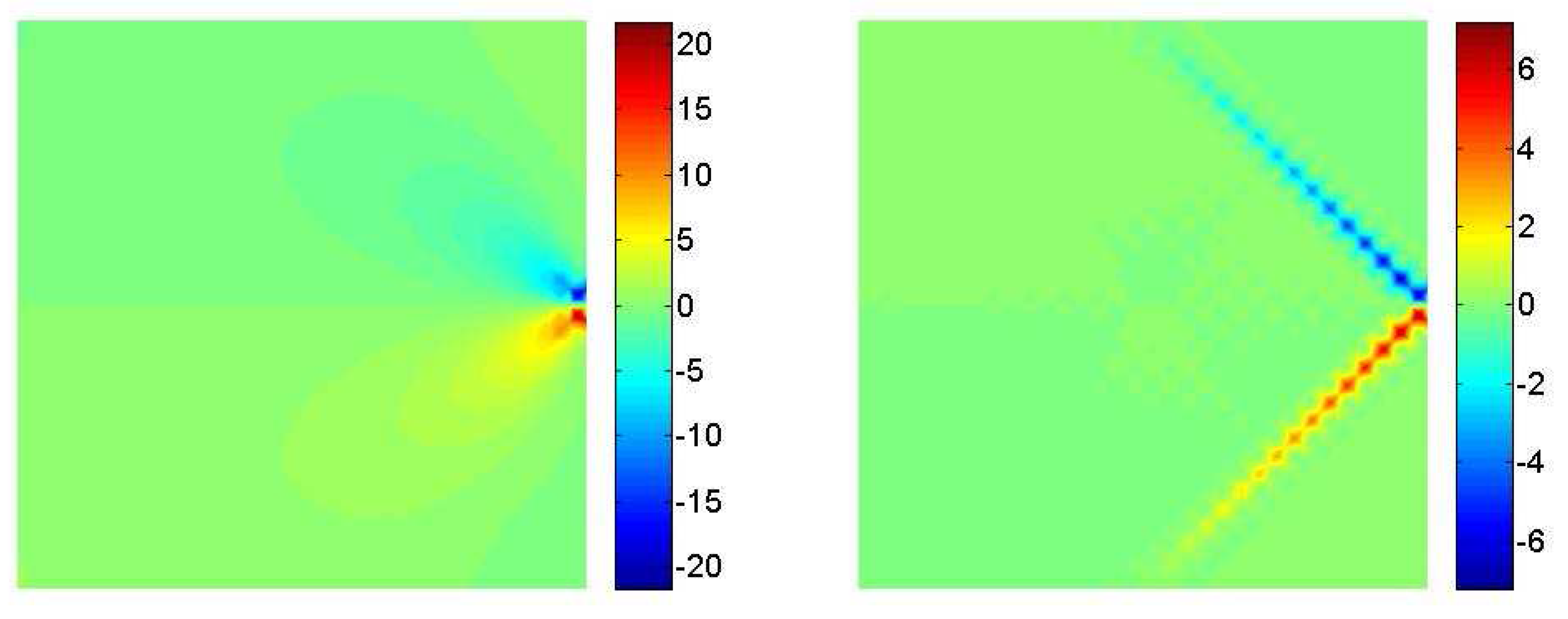
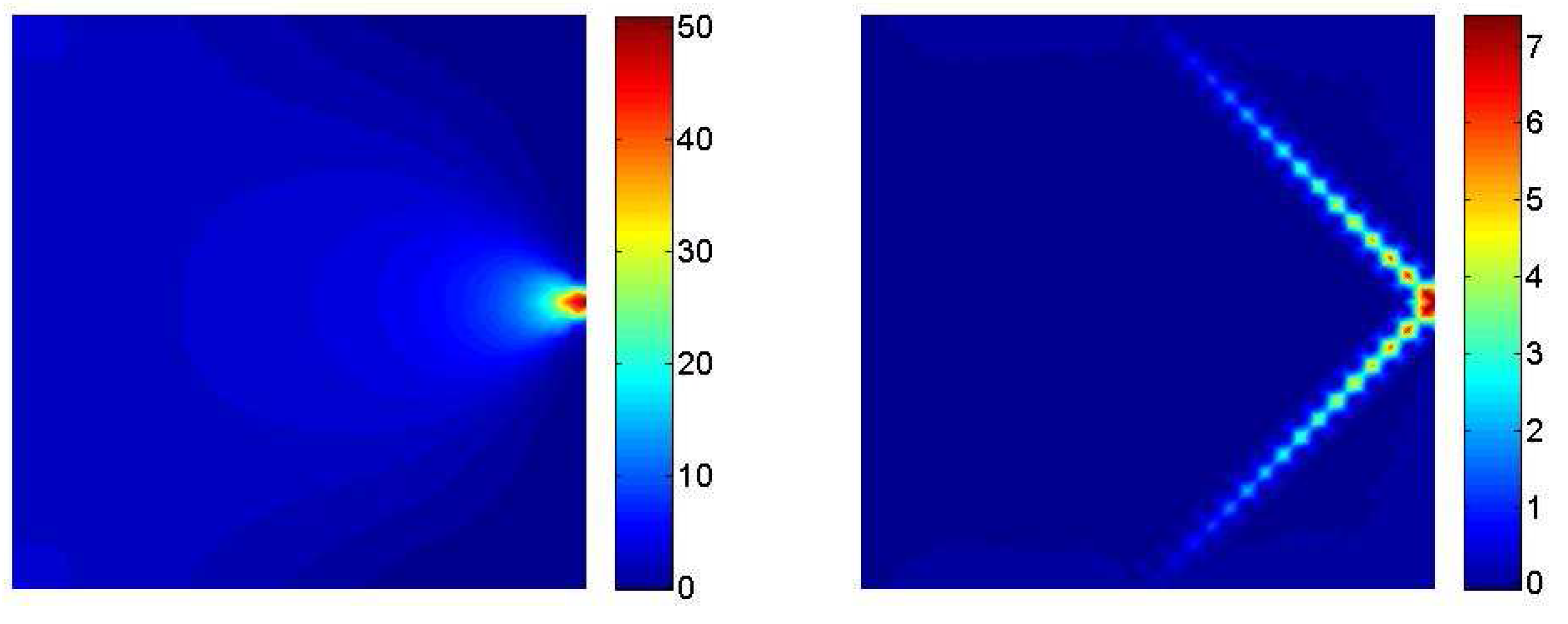
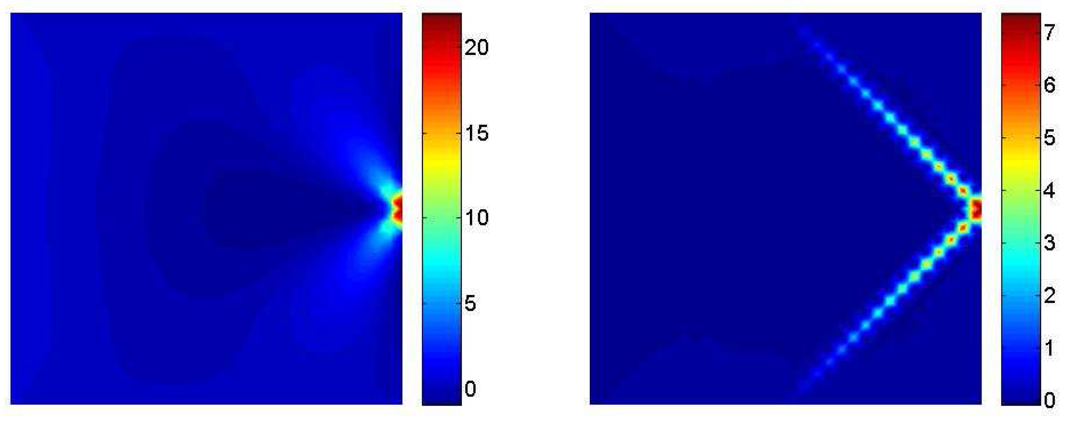
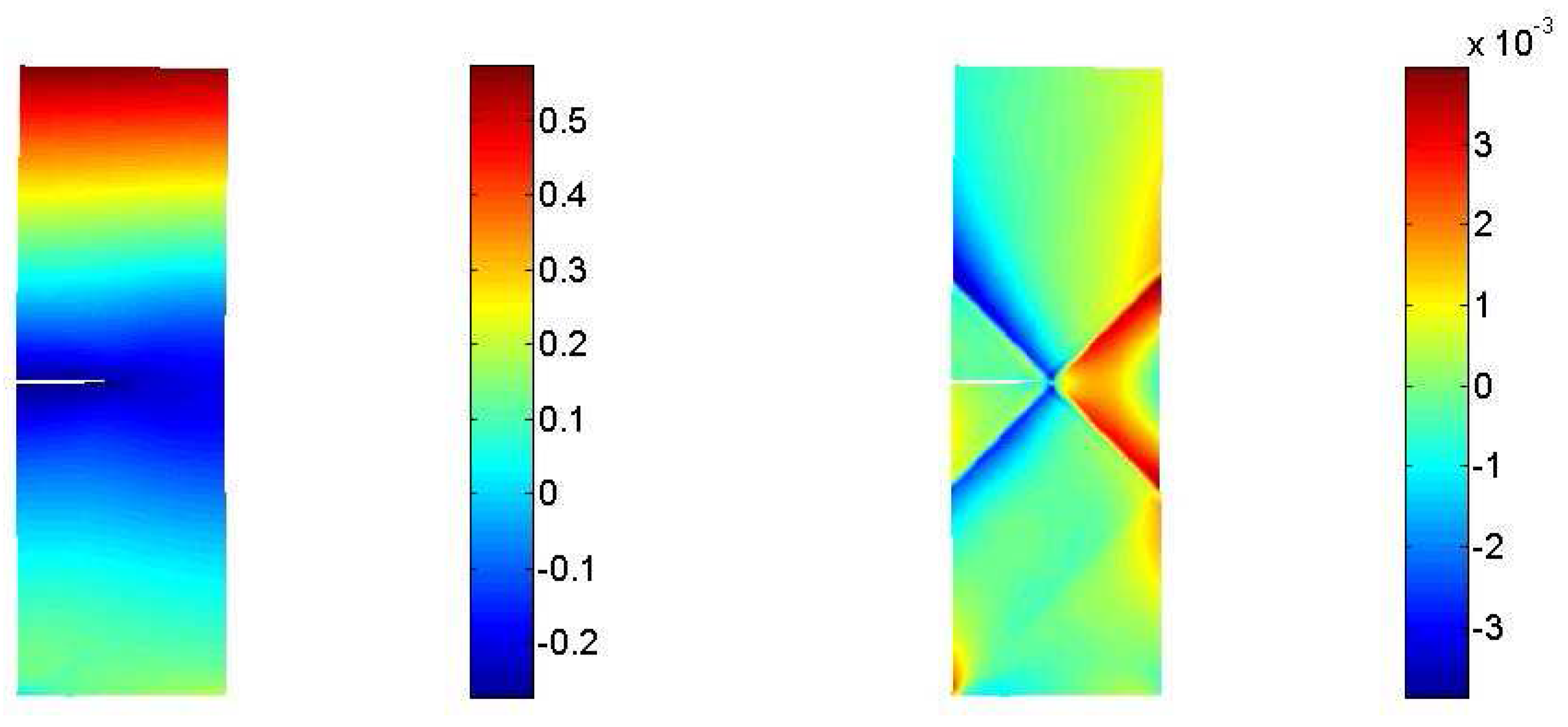
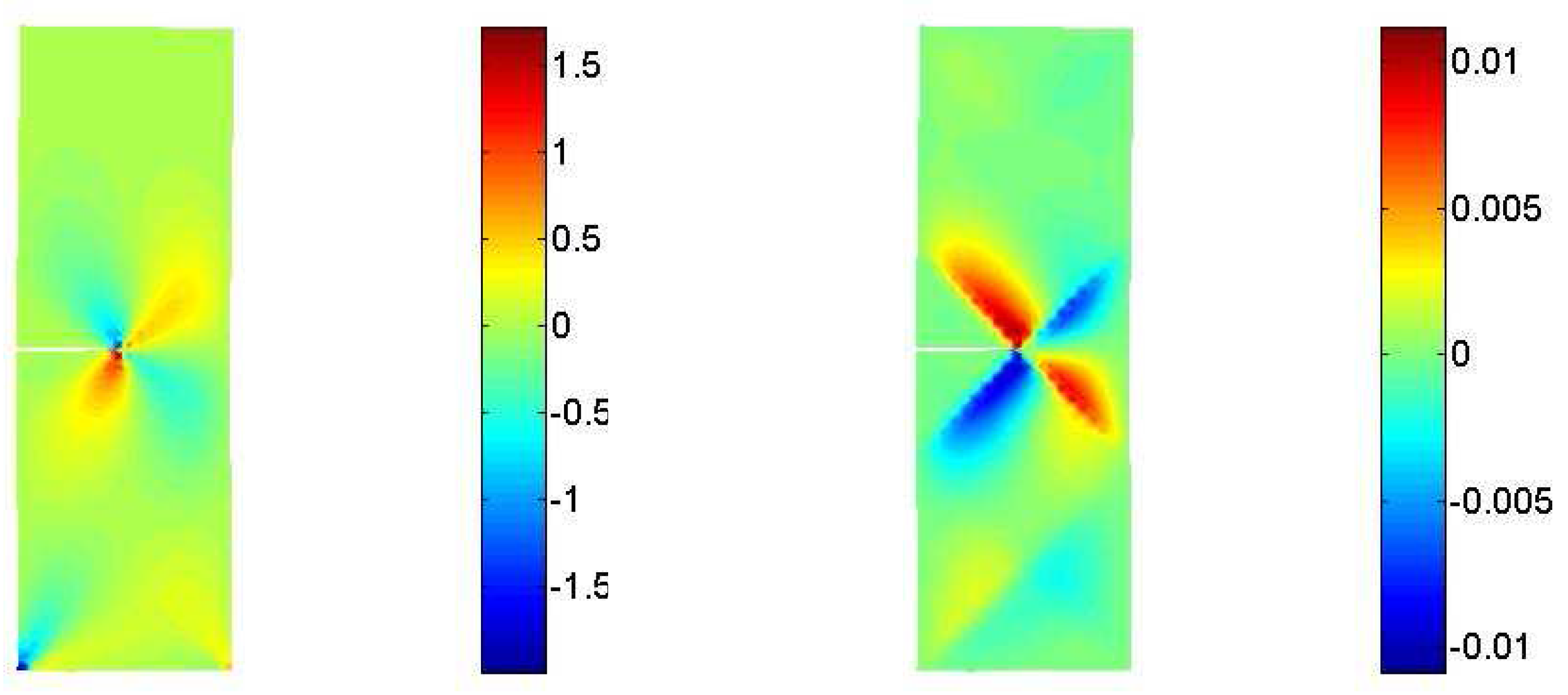
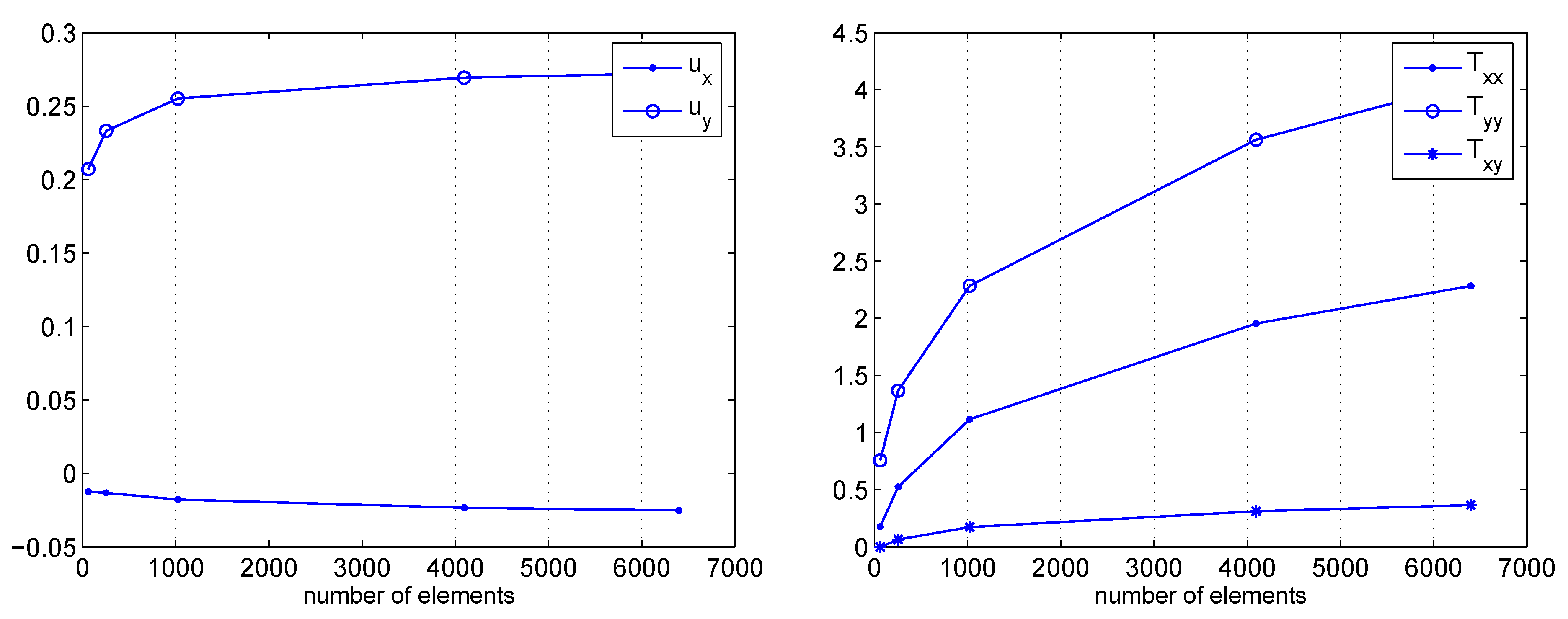
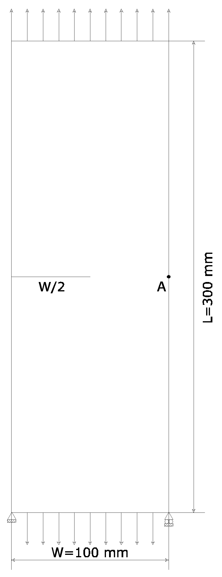
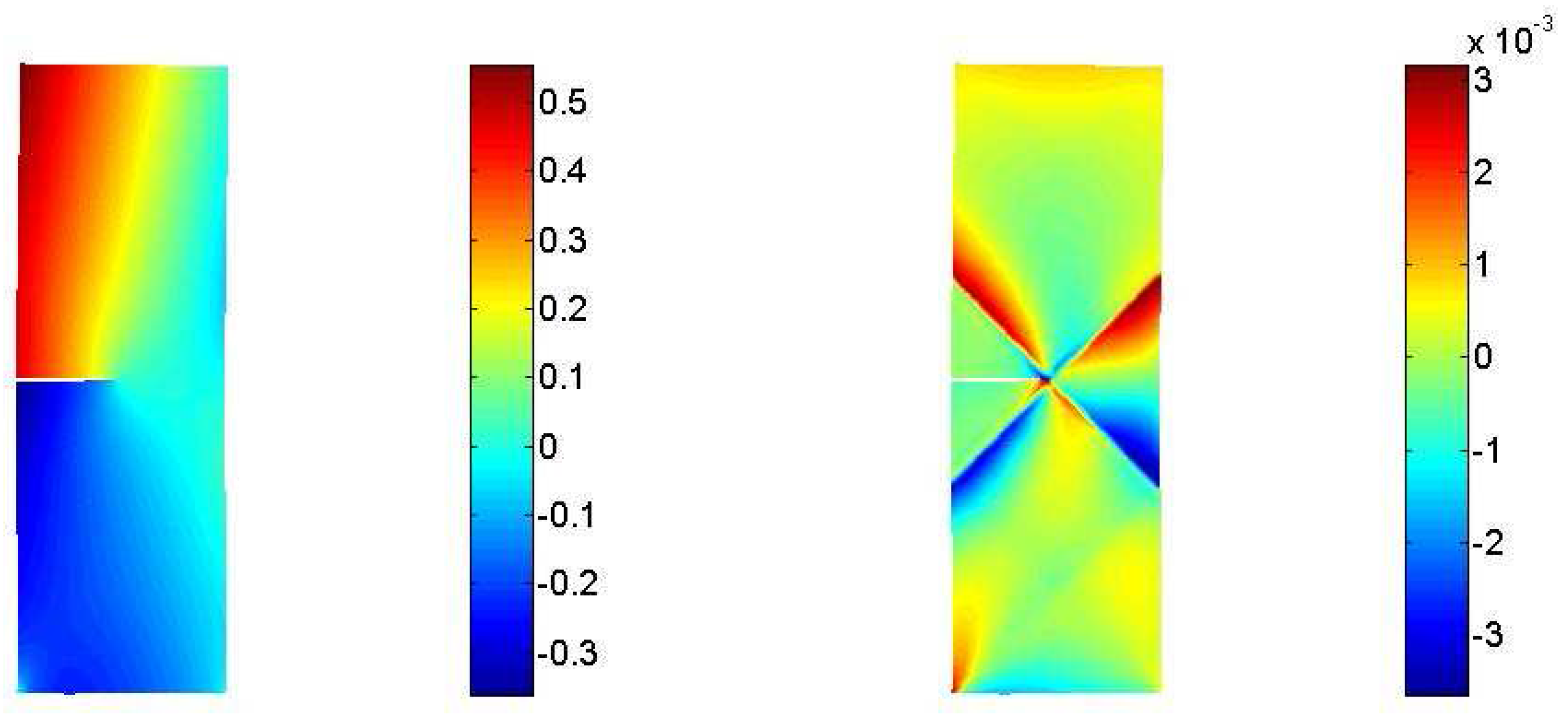
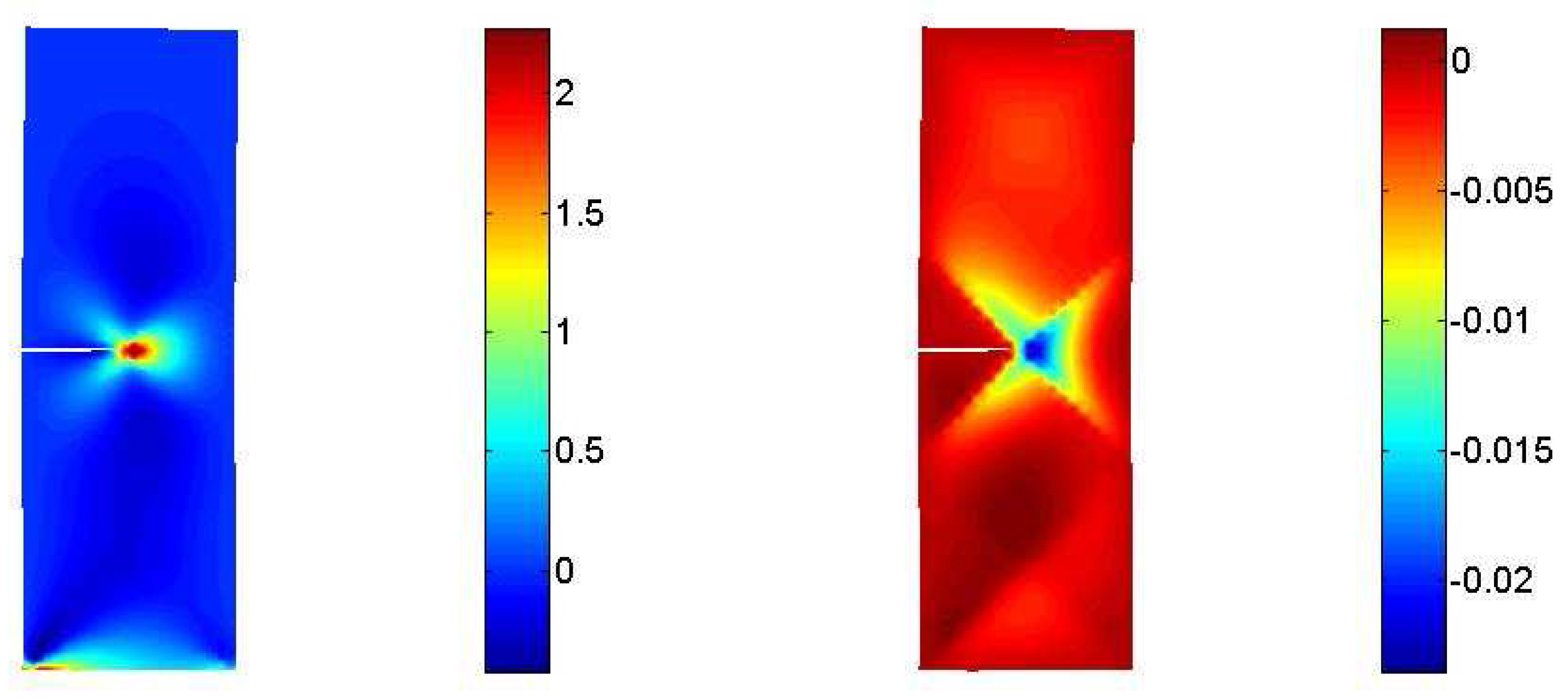
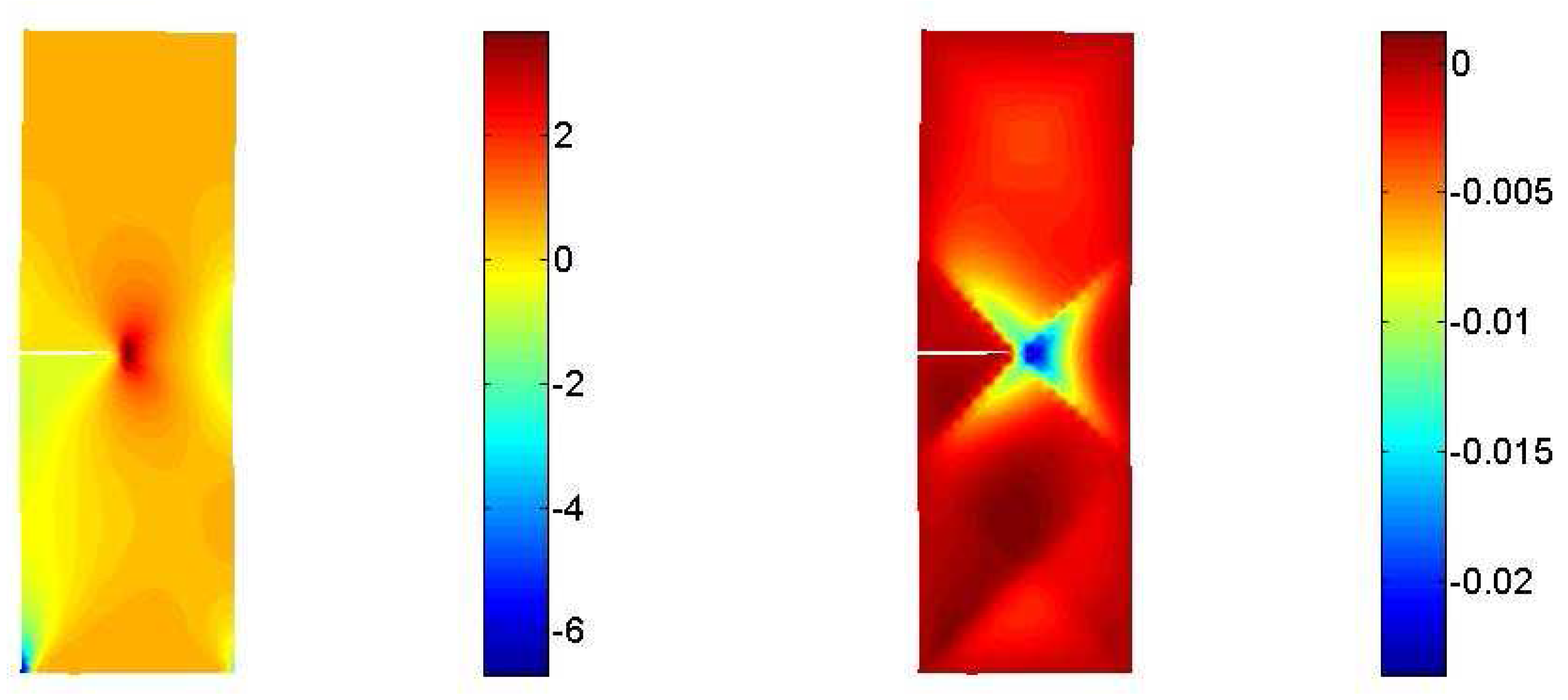
3.2. Interaction between a macrocrack and diffuse microcracks

To study the effect of the presence of a macrocrack in the microcracked domain we analyze the specimen of Figure 9, where a horizontal crack in the middle of the right side induces a geometrical singularity. The same example was originally investigated in [10], that used a variation of the well–known X–FEM methods to deal with the description of the macro–discontinuity embedded in the microcracked medium. The mechanical parameters, as declared in [10], are reported in Table 3.2. for completeness sake. Boundary conditions refer in this case to the only macro displacements field, as straightforwardly derived from a classical description of the Cauchy type.
Table 2. Physical parameters.
m [ m m ] M [ m m ] E [ N / m m 2 ] A [ m m 2 ] A ^ [ m m 2 ] C m m χ
755 10 3 10.0314150
Figure 9. The cracked plane membrane.
Algorithms 02 00606 g009
As detailed in the original contribution [10], macro displacements are not affected by any localization phenomenon. A remarkable concentration conversely characterizes the micro vectors, see Figure 10 and Figure 11. The geometrical singularity, i.e. the crack tip, activates a 45–degree displacement localization that has the shape of a regular four–brace cross arising in the vicinity of the tip.
Figure 10. Macro–displacements u x - Micro–displacements d x .
Algorithms 02 00606 g010
Figure 11. Macro–displacements u y - Micro–displacements d y .
Algorithms 02 00606 g011
Figure 12, Figure 13 and Figure 14 show plots of both the macro and micro stress tensors on the whole domain. The macro stress diagrams show results that are well–known within the field of fracture mechanics for classical Cauchy media. The performed numerical analysis capture the macro stress concentration that typically arises at the tip of a cohesive fracture. It is quite interesting to notice that the micro displacement localizations have a counterpart in the micro stress field. All the components of the micro stress tensors are affected by a remarkable localization in the vicinity of the crack tip. In this case the magnitude of the micro quantities is lower than the macro ones and one may conclude that the macro singularities due to the crack tip overcome the localization phenomena peculiar to the micro level.
The example is also used to introduce some preliminary investigations on the convergence properties of the adopted mixed discretization with respect to the macro and micro variables that have been directly discretized in the model. To this purpose the point A, located in the middle of the vertical right side of the specimen, has been firstly used to draw the convergence curves plotted in Figure 15 and Figure 16. The point A is also represented in Figure 9.
Figure 12. Macro–stress T x x - Micro–stress S x x .
Algorithms 02 00606 g012
Figure 13. Macro–stress T y y - Micro–stress S y y .
Algorithms 02 00606 g013
Figure 14. Macro–stress T x y - Micro–stress S x y .
Algorithms 02 00606 g014
At a first glance the diagrams point out that all the numerical unknowns of the methods, i.e. two macro displacement vectorial components u x and u y , two micro displacement vectorial components d x and d y , three macro stress tensorial components T x x , T y y and T x y , three micro stress tensorial components S x x , S y y and S x y , approximately enjoy a similar convergence rate. This is mainly due to the adopted mixed polynomial discretization, see i.e. Section 2.1.. Improvements in the accuracy of the results, especially for what concerns the stress interpolation, may be straightforwardly achieved by the adoption of finer polynomial interpolations. One may also resort to the dual formulation of Section 2.2., which principally takes advantage of the role of the stresses that are discretized as main variables of the problem.
Figure 15. Point A. Macro–displacements convergence - Micro–displacements convergence.
Algorithms 02 00606 g015
Figure 16. Point A. Macro–stresses convergence - Micro–stresses convergence.
Algorithms 02 00606 g016
Additional remarks on convergence issues may be derived investigating the behavior of the mixed discretization in the vicinity of the crack tip, where an accurate prediction of the stress field is often an hard challenge for finite element schemes. Figure 17 presents convergence curves for both macro quantities, i.e. the displacement vector and the stress tensor. Notwithstanding the coarse mixed polynomial interpolation herein implemented, the mixed scheme is able to capture the components of the displacements vector with a convergence rate that is very similar to the one previously highlighted for point A. The convergence of the stress tensor components is more difficult, since finer discretizations must be used to achieve the highest accuracy. However the convergence curve remains smooth all over the considered range and clearly tends to the expected plateau without the arising of any numerical instability. These results may be considerably improved by the adoption of the "truly–mixed" scheme of Section 2.2., that should exhibit a very fast convergence in terms of the stress intensity factor (SIF) or any other scalar measure of the stress field at the crack tip. The role of the stresses as main variables of the problem is expected in this case to assure better prediction, especially in the singularity zone.
Figure 17. Crack tip. Macro–displacements convergence - Macro–stresses convergence.
Algorithms 02 00606 g017

4. Conclusions and future work

The paper has dealt with the numerical description of microcracked bodies according to the theories introduced in [9,10] and belonging to the framework of multifield continua [5]. Two extensions of the mixed variational formulations descending from the principle of Hellinger Reissner have been herein presented, taking also into account the inclusion of macrocracks within the microcracked model.
A few numerical investigations have been illustrated in order to assess the capabilities of the method to cope with localization phenomena that affect not only the displacement field but also the stress one. These simulations, based on the first of the two methods herein presented, may be considered as preliminary investigations to test the accuracy of the interpolations when handling a macro and a micro level. It must be remarked that the introduction of a mixed discretization requires a larger number of unknowns with respect to classical displacement–based interpolations. Notwithstanding the increased computational burden this allows to provide a better accuracy in the description of the stress field, that is not derived through any post–processing technique, since it is one of the unknowns of the problem. This is a remarkable feature especially in the case of the herein considered multifield approach, where a high accuracy is required to properly capture the expected localization phenomena.
The current research is focused on the the features of the "truly–mixed" scheme, to implement numerical methods that exploit the advantages of a problem description where stresses are the main variables. As emphasized in the paper, this allows to further improve the accuracy of the method and to tackle, in a more straightforward way, problems as the inclusion of a macrocrack within a continuous body.

Acknowledgements

The inspiring contribution of Professor Paolo Maria Mariano is gratefully acknowledged.

References and Notes

  1. Arnold, D.N.; Brezzi, F.; Douglas, J.D. PEERS: a new mixed finite element for plane elasticity. Japan Journal of Applied Mathematics 1984, 1, 347–367. [Google Scholar]
  2. Brezzi, F.; Fortin, M. Hybrid and Mixed Finite Element Methods; Springer: New york, 1991. [Google Scholar]
  3. Bruggi, M.; Venini, P. A Truly Mixed Approach for Cohesive–Crack Propagation in Functionally Graded Materials. Mechanics of Advanced Materials and Structures 2007, 14, 643–654. [Google Scholar]
  4. Bruggi, M.; Venini, P. A mixed FEM approach to stress-constrained topology optimization. International Journal for Numerical Methods in Engineering 2008, 73, 1693–1714. [Google Scholar]
  5. Capriz, G. Continua with microstructures; Springer Tracts in Natural Philosophy, 35; Springer: Berlin, 1989. [Google Scholar]
  6. Johnson., C.; Mercier, B. Some equilibrium finite elements methods for two dimensional elasticity problems. Numer: Math. 1978, 30, 103–116. [Google Scholar]
  7. Krajcinovic, D. Damage mechanics; North-Holland: Amsterdam, 1996. [Google Scholar]
  8. Mariano, P.M. Multifield Theories in mechanics of solids. Adv. Appl. Mech. 2002, 38, 1–93. [Google Scholar]
  9. Mariano, P.M.; Stazi, F.L. Strain localization in elastic microcracked bodies. Comp. Methods Appl. Mech. Engrg. 2001, 190, 5657–5677. [Google Scholar]
  10. Mariano, P.M.; Stazi, F.L. Strain localization due to crack-microcrack interactions: X-FEM for a multifield approach. Comp. Methods Appl. Mech. Engrg. 2004, 193, 5035–5062. [Google Scholar]
  11. Moës, N.; Belytschko, T. Extended finite element method for cohesive crack growth. Engineering Fracture Mechanics 2002, 69, 813–833. [Google Scholar]
  12. Schenk, O.; Gärtner, K. Solving Unsymmetric Sparse Systems of Linear Equations with PARDISO. Journal of Future Generation Computer Systems 2004, 20, 475–487. [Google Scholar]
  13. Schenk, O.; Gärtner, K. On fast factorization pivoting methods for symmetric indefinite systems. Elec. Trans. Numer. Anal. 2006, 23, 158–179. [Google Scholar]
  14. Torquato, S. Random heterogeneous materials; Springer Verlag: Berlin, 2002. [Google Scholar]

