Neural Network Modeling to Predict Shelf Life of Greenhouse Lettuce

Abstract

Greenhouse-grown butter lettuce (Lactuca sativa L.) can potentially be stored for 21 days at constant 0°C. When storage temperature was increased to 5°C or 10°C, shelf life was shortened to 14 or 10 days, respectively, in our previous observations. Also, commercial shelf life of 7 to 10 days is common, due to postharvest temperature fluctuations. The objective of this study was to establish neural network (NN) models to predict the remaining shelf life (RSL) under fluctuating postharvest temperatures.  A box of 12 - 24 lettuce heads constituted a sample unit. The end of the shelf life of each head was determined when it showed initial signs of decay or yellowing. Air temperatures inside a shipping box were recorded. Daily average temperatures in storage and averaged shelf life of each box were used as inputs, and the RSL was modeled as an output. An R² of 0.57 could be observed when a simple NN structure was employed. Since the “future” (or remaining) storage temperatures were unavailable at the time of making a prediction, a second NN model was introduced to accommodate a range of future temperatures and associated shelf lives. Using such 2-stage NN models, an R² of 0.61 could be achieved for predicting RSL. This study indicated that NN modeling has potential for cold chain quality control and shelf life prediction.

1. Introduction

Harvested lettuce heads should be stored at 0°C until marketed or used [1]. Research has shown that the shelf life of lettuce stored at 0°C is 21 - 28 days, but only about 14 days when stored at 5°C [2]. Pre-cooling and maintaining lettuce at low temperatures, without interruption, is one of the most important factors for prolonging post-harvest shelf life and quality. Shelf life of field-grown lettuce was prolonged by rapid (vacuum) cooling immediately following harvest [3]. If pre-cooled lettuce is left outdoors at an air temperature of approximately 21°C, the core temperature can go from 0.6°C to 10°C within the same day [4]. Greenhouse-grown butterhead lettuce is more perishable than field-grown iceberg lettuce [5]. Our preliminary results indicated that vacuum cooling improved the shelf life of commercially harvested greenhouse lettuce [6].

Temperature fluctuations during post-harvest handling and storage also influence shelf life, and it is desirable to be able to predict the remaining shelf life (RSL) for a box of lettuce. For this reason, some type of device was necessary to record temperatures after harvest. There are two general approaches. First, time-temperature indicators (TTI) may be used to monitor temperatures and to predict shelf life. Three types of TTI for temperature-sensitive foods [7] were available based on; the melting point of a chemical mixture (e.g. 3M Monitor Mark), an enzymatic reaction (e.g. Vitsab TTI tags), or a polymerization reaction (e.g. LifeLines FreshCheck indicators). Some of these consumer readable TTI tags were evaluated with greenhouse-grown lettuce in a previous study, and Vitsab was found to be most suitable for lettuce [8]. There are certain problems that need to be corrected before TTI can be used [9]. For example, manual activation of the TTIs may cause variability in the mixing of the lipid substrate and the enzyme. A machine was designed to activate the TTIs automatically and uniformly in large-scale applications. Even more critical, the activation energy of food and the TTI must be identical, often requiring thorough experimentation. Secondly, a recording device such as a portable data logger can be placed inside a box of lettuce, and temperature records of shipping conditions can be retrieved at various points along the distribution chain. The total shelf life (TSL) of a lettuce head consists of the total number of remaining marketable days: the number of days in storage until the present, plus the RSL which consists of a sum of unknown days into the future. If the overall response of a product to variable storage temperature scenarios can be modeled, it should be possible to use measurements to a given date during the storage period to predict what will occur under assumed future conditions. However, the interactions of temperature and time are complex and difficult to model.

Methods to model and predict biological functions are often difficult due to non-linear responses and complicated interactions among input factors. A new approach, neural network (NN) modeling, has been applied to predict biological functions. NN models have been used for different predictions: canopy photosynthesis [10], shelf life of meat products [11], pepper fruit coloration [12], and pepper weekly yields [13]. There is no literature reporting the use of NNs to predict shelf life of greenhouse-grown lettuce. The objective of this study was to develop models for predicting RSL of greenhouse-grown lettuce. The data used were from experimental and commercial harvests involving a wide range of pre-harvest conditions and post-harvest temperature fluctuation. Several NN models were established and validated against observed shelf lives. Regression analysis was also used as a comparison.

2. Description of Neural Network

The mathematical description of 2-stage backward propagation neural networks (BPNN) consists of definition of shelf life, structure of generic BPNN, heuristic approaches, and application of NN model for shelf life prediction. The theory and applications of NNs were described by Baughman and Liu [14].

The definition of shelf life. We collected data of total shelf lives from a number of units of lettuce grown experimentally or commercially. Each unit (box) of lettuce has its own history of average daily temperatures. In this study, shelf life is defined as average shelf life (days) of a box of lettuce with 12-24 heads. The criteria for determining shelf life must be consistent for all the units and all sources of harvest. Given this data, we are required to build a model to predict the RSL. The question is “For this unit of produce with known daily average temperature history up-to-today, what RSL (days) can be expected under various scenarios of future temperatures?”

Generic BPNN. Generic NN models for modeling RSL can be expressed as a function of the product of a weight matrix W and input vector T,

[RSL = f(W*T)]

(1)

where W is a resulting BPNN weight matrix, T represents the temperature history, and RSL is the remaining shelf life. The number of points of temperature data in a given unit is the same as the number of days of total shelf life, and each unit has its own total shelf life. The dimension of input vector T (the number of input nodes) is fixed in a given BPNN model. In order to accommodate the varying number of total shelf lives, the input vector T was the average daily temperature for each unit. For example, a maximum of 18 daily temperature inputs are possible for a box of lettuce observed having 18 days of shelf life.

If the temperature history of a unit has a total shelf life of n days, the daily temperatures are t(1), t(2), …, t(c), …, t(n). The c in t(c) indicates the current day (“today”) as it moves from t(1) to t(n) along the time axis. The components of vector T, i.e. the input nodes for current day (c), can be assigned as follows.

Input node fs (future sum): the sum of daily temperatures from tomorrow (c+1) to end of shelf life (n). This node fs covers the temperatures of the RSL of (n-c) days.

[fs = t(c+1) + t(c+2) + … + t(n)]

(2)

Input node fa (future average): the average daily temperature of the remaining days (n-c).

[fa = fs / (n-c)]

(3)

Input nodes pm: one node for each of the previous m days counting back from day c: For example, If m=4 days, then we are using t(c), t(c-1), t(c-2) and t(c-3) as inputs.

[pm = {t(c), t(c-1), t(c-2), …, t(c-(m-1))}]

(4)

Input node ps (prior sum): the sum of daily temperatures prior to day (c-(m-1)).

[ps = t(1) + t(2) + … + t(c-m)]

(5)

The output node, RSL, for a given day c is simply described as:

[RSL = n-c]

(6)

This design is one of numerous possibilities, and allocating the up-to-date temperatures into aggregates of nodes (i.e. pm) is an art. In our design of nodes pm, we emphasize the details of temperatures in the last m days (i.e. immediately before current day (c)), assuming that the last m days of temperature may be most important. We used a summation (ps) as a single node for the temperatures prior to day (c-(m-1)).

Heuristics. NN models are established by learning from examples (i.e. available data set), but they can not provide in-depth solutions (i.e. no explanation capacity). On the other hand, knowledge-based expert systems can not easily process information from real-life, unpredictable data. A hybrid structure of expert systems and neural networks has been proposed and implemented in bioprocessing and chemical engineering [14] (section 6.1 Introduction to Expert Networks, pp. 365-369). The knowledge gained from those studies using TTIs in postharvest handling provides us with the basis for incorporation of the following heuristics into NN models [8,9].

Heuristics #1:

The set of nodes of vector T so designed includes fs, fa, pm, and ps. The nodes fs, pm, and ps are simply aggregates of the temperature history in storage. The node fa is introduced in order to allow us to make the RSL prediction more meaningful to end-users. For example, we will be able to interrogate the 2-stage NN model by varying fa in selected intervals of temperature to get the corresponding range of RSL (Heuristics #2, below).

Heuristics #2:

Once the BPNN model is established, we can use its resulting matrix W to determine RSL from equation (1), RSL = f(WT), for a real-life T and given day c. The vector T is expressed as T = (ps, pm, fa, fs).

Here we are immediately faced with the difficulty of unknown fs, since we do not know what the future storage temperatures will be. During the training stage there is no such difficulty, since node fs in vector T is available and well defined from the given historical training data. From the definitions it is obvious that fs, fa, and RSL are mutually dependent via the factor (n-c). Superficially, the node fs is proportional to fa simply by the factor of (n-c). However, the factor (n-c) is the RSL itself which also depends on the temperature history, viz., ps, pm, and fs. Thus we have to introduce the Heuristics #2 as follows.

The future sum (fs) of temperatures is obtained by an auxiliary BPNN:

[fs = f(YS)]

(7)

where the vector S is defined as S = (ps, pm, fa), and the matrix Y is just another weight matrix obtained from the auxiliary BPNN.

In other words, we are making a good estimate of fs via this auxiliary BPNN using weight matrix Y.

Then we have a heuristic 2-stage BPNN model in order to predict the RSL:

Stage 1; obtain fs using the following:

S = (ps, pm, fa)

fs = f(YS)

Stage 2; input fs into T and obtain RSL by using:

T = (ps, pm, fa, fs)

RSL = f(WT)

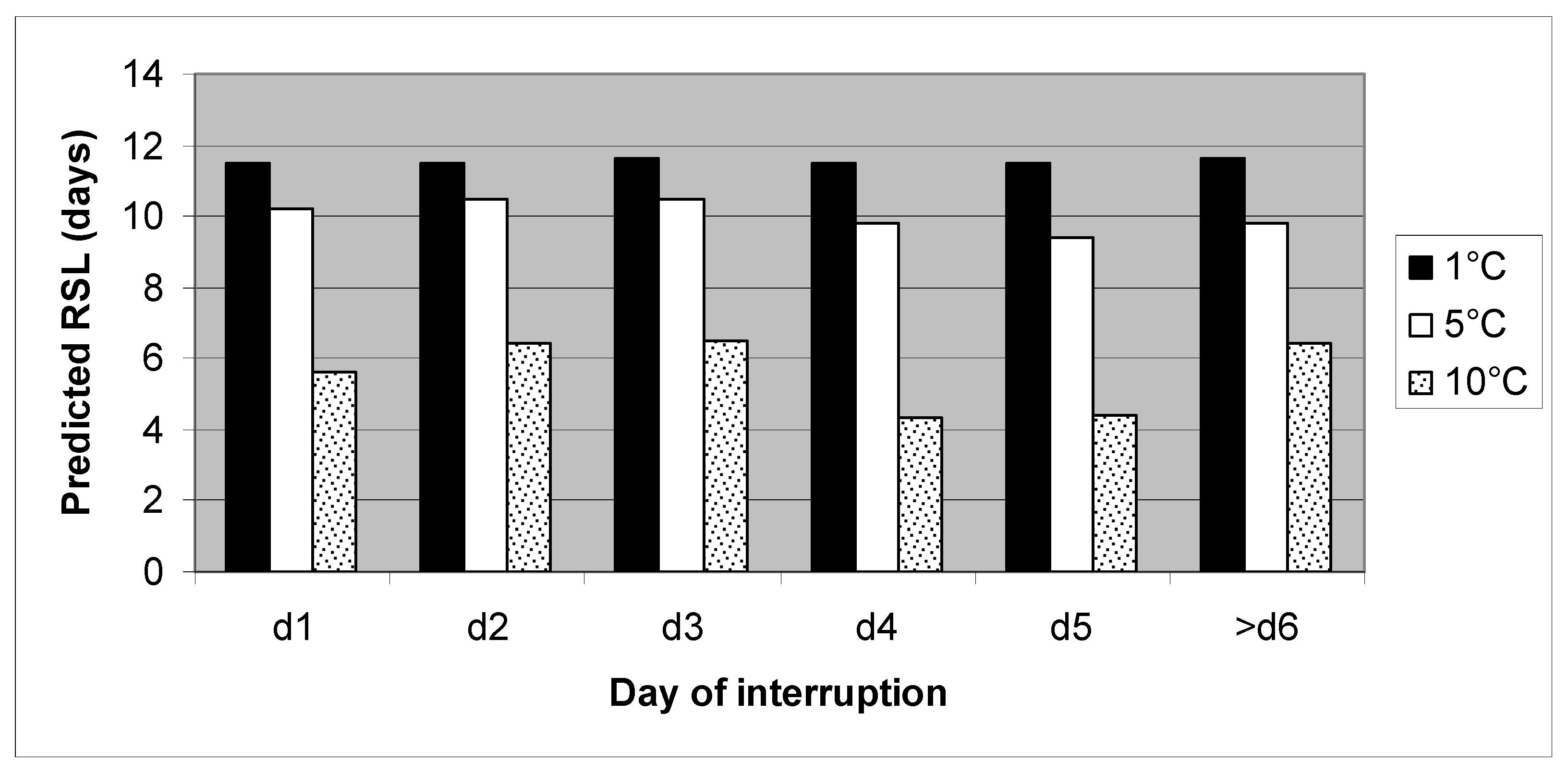
In short, we used stage 1 of BPNN to establish the relationship between RSL and fa on the basis of existing historical data. Once the relationship between RSL and fa is established, the RSL can be predicted in stage 2 of BPNN according to a user-specified range of future storage temperature (i.e. fa). In so doing, the predicted RSL is more realistic to commercial practice and tailored to end-user’s specific postharvest conditions. For example, the end-user can ask what the RSL would be if a box of lettuce is placed in a 4°C refrigerator, or what the RSL would be in the retailers’ holding area at 10°C?

Application. In building a 2-stage NN, we separately train BPNN matrices Y (of stage 1) and W (of stage 2) according to the scheme of input vector sets S and T, respectively, for given training data. The same convergence criteria must be used in selecting Y and W. The convergence criteria used in model training includes R-square, root-mean-square and coefficient of variation (CV) for the output node RSL. During model training, we select the same optimal cycle number for both weight matrices Y and W. A special computer program was developed in this study to integrate stage 1 and stage 2 into one operation for end users. Once a model has been trained, the end-user can specify a discrete set of fa values inside a selected temperature interval to obtain corresponding RSL values.

3. Materials and Methods

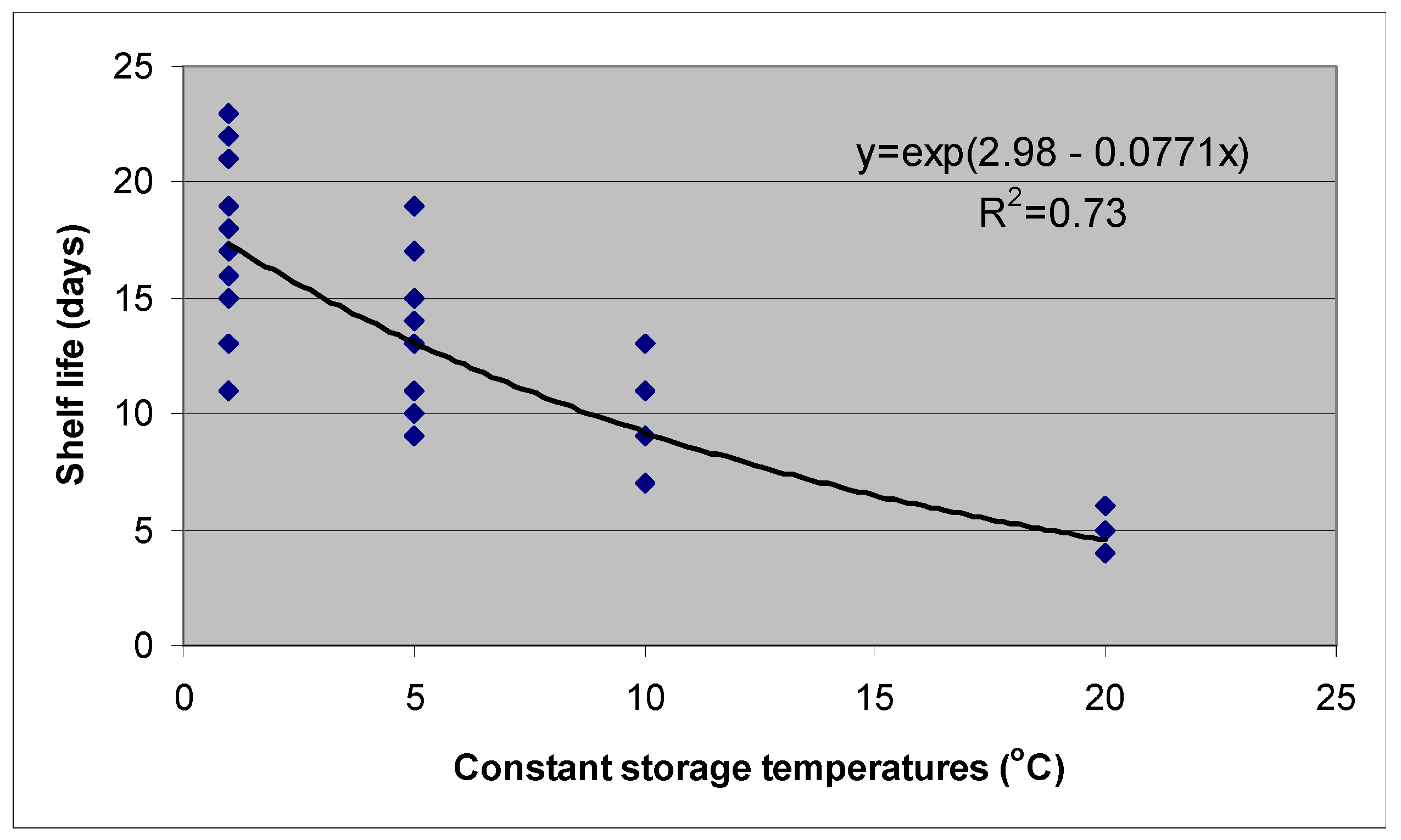
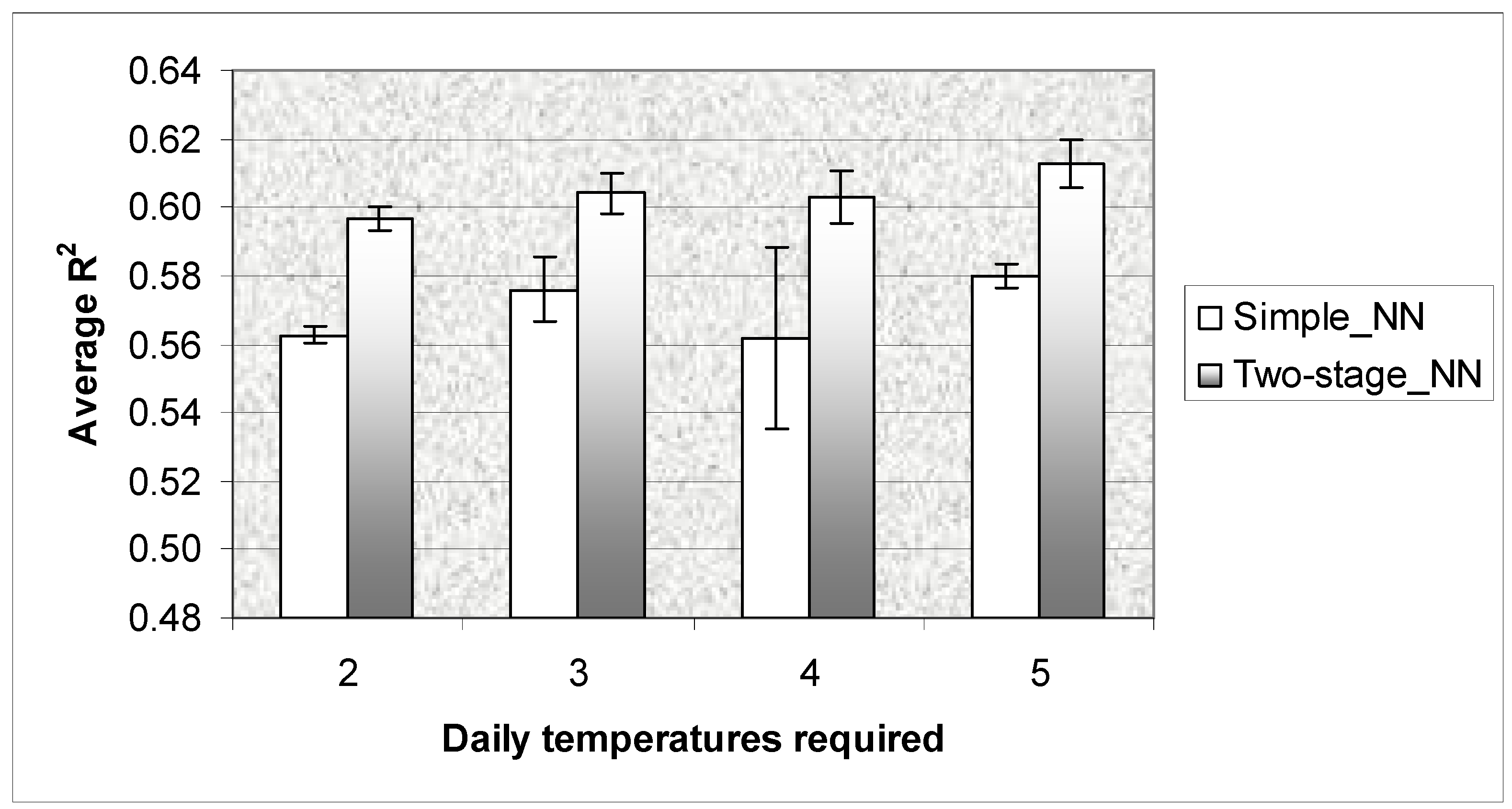
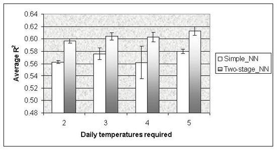
Plant materials. Plants of butterhead lettuce cvs Cortina and Prior were grown under experimental conditions in Agassiz or obtained from a commercial greenhouse in Pitt Meadows, both located within 100 km east of Vancouver, British Columbia, Canada. The experimental plants were harvested from 8 experiments. Butterhead lettuce cv. Prior was used: 6 experiments involved living lettuce (with trimmed roots) and another 2 experiments used butter lettuce (with no roots). These experiments covered various pre-harvest growing conditions and post-harvest temperature combinations (details not shown). Six commercial harvests were obtained directly from the commercial greenhouse. There were 8 experiments involving cvs. Cortina and Prior, including living and butter lettuce. The same postharvest procedures were applied to experimental and commercial materials. Storage experiments were conducted in Agassiz. Living lettuce retains a partial root system, while butter lettuce has the root system removed upon harvest. Each head of living or butter lettuce was wrapped individually with a plastic sleeve. There were 12, 18 or 24 heads in a box. Each box was considered as an experimental unit. There were a total of 198 boxes, including both experimental and commercial harvests. The air temperature of each box was recorded by a portable Hobo Temperature Data Logger, model H08 (Onset Computer Corp. Bourne, MA 02532, USA). Temperatures were averaged over a 24-hour period until shelf life was terminated. Total shelf life of each head is defined as the number of days between date of harvest and the date a lettuce head shows incipient yellowing or decay. Each head of lettuce was visually inspected 3 times a week. The incipient signs of yellowing and decay caused a lettuce head to be considered as unmarketable by the industry in British Columbia. The remaining shelf life (RSL) of each box was the average of 12, 18 or 24 heads, and used as output for shelf life prediction. At the end of each storage experiment, the RSL was back calculated by using the difference between the total shelf life (n) and the number of days in storage until current day (c). In training and testing of simple and 2-stage NN models, a total of 198 data cases were used, representing 198 boxes of lettuce harvested during 1998-2001. Routinely, 80% of 198 cases were randomly selected for training NN models and the remaining 20% were put aside and later used for testing the models. A good fit for NN models was determined by high R² values and low average errors (%) in testing. Randomization of the selected training cases was repeated at least once. The testing was arbitrarily stopped when R² of two consecutive results were within 10% or less. Further, the same experimental data used for establishing NN models was used to train regression models, and identical commercial data was used to validate both 2-stage NN and regression models.

Simple NN models. In simple NN modeling daily storage temperatures were used directly to model RSL, while future temperatures were assumed not yet available and ignored. A simple NN model was established by using past daily temperatures with two manipulations. First, the last daily temperature t(c) and backward preceding m daily temperatures (pm) expressed as t(c), t(c-1), t(c-2), …., t(c-(m-1)) were used as input pm nodes for the NN model. Secondly, daily temperatures before t(c-m) were totalled as temperature_prior_sum (ps). The values of ps and pm were used as inputs for modeling RSL. In BPNN, we generated a set of vectors T from the given data set containing a number of units, in which each unit has its own history of storage temperatures and its own total shelf life (n). We then performed the training procedures accordingly. For each unit, we ran the given day c from day 1 to day n, and generated n number of T vectors (e.g. shelf life of 18 days gave 18 T’s; each of 18 T’s had its own RSL as defined by n-c). Each vector T contained the input nodes, pm and ps, along with the associated output node, RSL, for a given day c. The BPNN of RSL consisted of three layers: the input layer, the intermediate layer, and the output layer. The input layer had nodes for pm and ps; the output layer had only one node, the RSL. The intermediate layer had a total number of nodes which is less than half of the sum of the input and output nodes. This simple NN procedure was described previously [12,13].

Two-stage (2-stage) NN models. In order to overcome the dependence of RSL on unknown future temperatures in simple NN models, a 2-stage NN procedure was employed. Unknown future temperatures were first modeled by an auxiliary NN in stage 1 using historical temperature records, and then combined with daily storage temperatures in a second NN in stage 2 to predict RSL in one operation. In stage 1, we established the temperature matrix S by using ps, pm, and fa, and modeled fs by using S and weight matrix Y (equation (7)). In stage 2, we used the resulting fs as part of temperature matrix T (ps, pm, fa, fs), and RSL was modeled as weight matrix W x T (equation (1)). In short, the auxiliary NN was established to model the relationship between future temperature sum (fs), future temperature average (fa) and RSL. This relationship was used to provide inputs for the second stage of the 2-stage NN to predict RSL.

Regression. The RSL was regressed with daily temperatures by using S-Plus (S-PLUS 6 for Windows, Release 1, Insightful, Seattle, WA). The predicted shelf lives were compared with those of 2-stage NN models. Identical data sets were used for 2-stage NN modeling and regression analysis.

4. Results and Discussion

4.1. Storage temperatures

In experimental crops, as constant storage temperature increased from 1°C to 20°C, the TSL of living lettuce decreased exponentially from an average of 18 days to 5 days (Figure 1). This was similar to our previous observations of TSL of 20, 14, 10 and 5 days under constant 1°C, 5°C, 10°C and 20°C, respectively, in one study [8] and 19, 10 or 6 days under constant 1°C, 10°C, and 20°C, respectively, in another [6]. There are two implications seen with storage at constant temperatures. First, even under constant storage of 1°C or 5°C, the observed TSL varied substantially (Figure 1). This may be attributed to pre-harvest factors such as the seasonal effects observed in this study. Secondly, in commercial practice, postharvest temperatures always vary throughout the distribution chain, and modeling on the basis of constant storage temperatures may not be suitable to commercial reality. This set of data indicated the need for a new approach to modeling shelf life of greenhouse lettuce which will include variable temperature scenarios. Among various approaches, neural networks were selected for this study. The use of neural networks has been suggested for modeling apple fruit quality in variable temperature scenarios [15].

Figure 1. Total shelf life (y-axis) of living lettuce was affected by constant storage temperatures of 1°, 5°, 10° or 20°C (x-axis). The exponential equation was based on Proc NLIN of SAS software package (SAS 9.1.3, 2002-2003 release; SAS Institute Inc., Cary, NC).

Figure 1. Total shelf life (y-axis) of living lettuce was affected by constant storage temperatures of 1°, 5°, 10° or 20°C (x-axis). The exponential equation was based on Proc NLIN of SAS software package (SAS 9.1.3, 2002-2003 release; SAS Institute Inc., Cary, NC).

4.2. Simple NN

In simple NNs, future temperatures were unavailable and ignored. Based on temperature records of all available 198 cases, simple NN models could predict RSL with average R² of 0.57 (Figure 2) when daily temperatures of 2 to 5 days were used. There was no statistical difference in R² between these four simple NN models. Many pre-harvest treatments such as light, air movement and nitrogen forms were imposed. For the post-harvest treatments, deviations from constant storage temperatures were also imposed: mainly, 1°C storage was interrupted with higher temperatures of 5°C or 10°C for 2-3 days in simulation of the commercial distribution chain as described by Prussia et al. [4]. Our data therefore ensured the broad data space which allowed for satisfactory predictions, but such diverse growing conditions also led to lower R² in those predictions. The necessity of using a broad data space was discussed previously in NN modeling of fruit coloration in greenhouse peppers [12]. Most commercial software packages can be conveniently used to establish simple NN models.

Figure 2. Ability of simple and 2-stage NN models to predict remaining shelf life (RSL) of living lettuce where model inputs include the current average daily temperature t(c) plus one to four average daily temperatures from 1, 2, 3 or 4 days prior to the current day. For example, “daily temperatures required” of 2 included t(c) and t(c-1), and the value 5 included t(c), t(c-1), t(c-2), t(c-3), and t(c-4). Good fit was indicated by higher R² in 2-stage NN (R²=0.61) compared to simple NN (R²=0.57) with LSD=0.016, according to the Proc GLM of SAS software package (SAS 9.1.3). Each bar represents a mean and its standard error obtained with testing of randomly selected testing data set. Each bar represents the mean of 2 to 4 tests.

Figure 2. Ability of simple and 2-stage NN models to predict remaining shelf life (RSL) of living lettuce where model inputs include the current average daily temperature t(c) plus one to four average daily temperatures from 1, 2, 3 or 4 days prior to the current day. For example, “daily temperatures required” of 2 included t(c) and t(c-1), and the value 5 included t(c), t(c-1), t(c-2), t(c-3), and t(c-4). Good fit was indicated by higher R² in 2-stage NN (R²=0.61) compared to simple NN (R²=0.57) with LSD=0.016, according to the Proc GLM of SAS software package (SAS 9.1.3). Each bar represents a mean and its standard error obtained with testing of randomly selected testing data set. Each bar represents the mean of 2 to 4 tests.

4.3. Two-stage NN

In 2-stage NNs, future temperatures were unavailable but were simulated first. Based on the same 198 cases used in simple NN, 2-stage NN models predicted RSL with average R² of 0.61 (Figure 2), when daily temperatures of 2 to 5 days were used. There was no statistical difference in R² between the four 2-stage NN models. Two-stage NN modeling has been used in many engineering processes [14]. When 1°C storage was interrupted with 5°C or 10°C on day 5, the RSL was shortened from 11 days to 9 or 4 days, respectively (Figure 3).

Figure 3. One-day interruption with 5°C or 10°C affected remaining shelf life (RSL) of 1°C stored living lettuce. On day 5, three sample cases which had storage temperature conditions of [1-1-1°C], [1-5-1°C], and [1-10-1°C] in sequence of [1d-3d-rest of storage] were used to interrogate 2-stage experimental NN model. The interruption during the first 5 days in storage was indicated by d1, d2, d3, d4, and d5. For day 6 onwards, the day of interruption is collectively indicated by >d6.

Figure 3. One-day interruption with 5°C or 10°C affected remaining shelf life (RSL) of 1°C stored living lettuce. On day 5, three sample cases which had storage temperature conditions of [1-1-1°C], [1-5-1°C], and [1-10-1°C] in sequence of [1d-3d-rest of storage] were used to interrogate 2-stage experimental NN model. The interruption during the first 5 days in storage was indicated by d1, d2, d3, d4, and d5. For day 6 onwards, the day of interruption is collectively indicated by >d6.

4.4. Validation and interrogation of 2-stage NN models

The 2-stage NN models based on data from experimental harvests could be validated with commercial harvests both in living and in butter lettuce. Living lettuce (with trimmed roots) and butter lettuce (with no roots) were expected to be different, and different models were established accordingly. For living lettuce, this study illustrated that the chosen experimental NN model could be validated with commercial harvests (Table 1), having R² of 0.66 and average error of 154%. The 2-stage NN models were used for interrogation. With all the data of living lettuce combined, storage temperatures recorded ranged from 1°C to 21°C. When fa of 1°C was assigned, most predicted RSL were longer than those actually observed (data not shown), and resulted in R² of 0.53 and average error of 212%. When fa of 21°C was assigned, most of the errors fell within 2 days of actual (Figure 4), and predictions resulted in R² of 0.65 and average error of 23%. Although there has never been any commercial practice to store lettuce at 21°C, this maximum temperature of 21°C did allow us to generate a reasonable range of potential RSL. Of course, any temperatures within the range of 1 – 21°C can be assigned to model and predict the RSL. As to butter lettuce, 2-stage NN models based on data from experimental harvests were validated by using a commercial harvest, having R² of 0.96 and average error of -34% (Table 1). When fa of 1°C was assigned, the R² was 0.95 and average error was -23%. When fa of 21°C was assigned, R² was 0.96 with average error of -66%. If we considered a predicted RSL that is within 2 days of its observed RSL as a useful criteria, 1°C resulted in a good prediction 6 out of 9 times, while 21°C generated only 3 good predictions out of 9 times. Two (2)-stage NNs confirmed the importance of a broad data base being used for training NN models, but with a penalty of having lower R². Living lettuce models were established with data from 66 cases covering 6 experiments over a 13-month period (Table 1), and butter lettuce models were established with 38 cases covering 2 experiments conducted in 2 months. The wider data space of living lettuce resulted in models with lower R² in commercial validation, whereas the NN models based on the narrow data range of butter lettuce resulted in models with higher R² in commercial validation.

Table 1. Validation of 2-stage NN experimental models with commercial harvests for predicting remaining shelf life (RSL in days) of living and butter lettuce.

Product types Z	Experimental model inputs	Validation with commercial harvests
		Cases W	Measure	Model validation	fa = 1°CU	fa = 21°CU
Living (n=66)	pm (m=3) Y, ps	28	R2	0.026	0.36	0.019
			Error (day)	4.5 (0.44)V	5.7 (0.39)	-0.2 (0.36)
			Error (%)	100% (10.8%)	136% (15.1%)	7% (6.1%)
	pm (m=5) X, ps	26	R2	0.66	0.53	0.65
			Error (day)	4.1 (0.32)	5.5 (0.39)	0.02 (0.29)
			Error (%)	154% (19.7%)	212% (26.6%)	23% (12.9%)
Butter (n=38)	pm (m=3) Y, ps	10	R2	0.89	0.92	0.81
			Error (day)	-1.8 (0.56)	-1.2 (0.66)	-3.7 (0.86)
			Error (%)	-25% (6.6%)	-16% (6.8%)	-59% (3.9%)
	pm (m=5) X, ps	9	R2	0.96	0.95	0.96
			Error (day)	-1.8 (0.49)	-1.6 (0.54)	-3.0 (0.64)
			Error (%)	-34% (6.1%)	-23% (9.6%)	-66% (2.5%)

^Z Product type: Individually wrapped lettuce with roots (living) or without roots (butter).^Y Refer to section “Generic BPNN” and equations (4) and (5). pm={t(c), t(c-1), t(c-2)} and associated ps.^X Refer to section “Generic BPNN” and equations (4) and (5). pm={t(c), t(c-1), t(c-2), t(c-3), t(c-4)} and associated ps.^W Number of validation cases in commercial data.^V Mean followed by standard error in bracket.^U Future average temperature (fa) was specified as 1°C or 21°C for 2-stage NN model interrogation.

Table 1. Validation of 2-stage NN experimental models with commercial harvests for predicting remaining shelf life (RSL in days) of living and butter lettuce.

Product types Z	Experimental model inputs	Validation with commercial harvests
		Cases W	Measure	Model validation	fa = 1°CU	fa = 21°CU
Living (n=66)	pm (m=3) Y, ps	28	R2	0.026	0.36	0.019
			Error (day)	4.5 (0.44)V	5.7 (0.39)	-0.2 (0.36)
			Error (%)	100% (10.8%)	136% (15.1%)	7% (6.1%)
	pm (m=5) X, ps	26	R2	0.66	0.53	0.65
			Error (day)	4.1 (0.32)	5.5 (0.39)	0.02 (0.29)
			Error (%)	154% (19.7%)	212% (26.6%)	23% (12.9%)
Butter (n=38)	pm (m=3) Y, ps	10	R2	0.89	0.92	0.81
			Error (day)	-1.8 (0.56)	-1.2 (0.66)	-3.7 (0.86)
			Error (%)	-25% (6.6%)	-16% (6.8%)	-59% (3.9%)
	pm (m=5) X, ps	9	R2	0.96	0.95	0.96
			Error (day)	-1.8 (0.49)	-1.6 (0.54)	-3.0 (0.64)
			Error (%)	-34% (6.1%)	-23% (9.6%)	-66% (2.5%)

^Z Product type: Individually wrapped lettuce with roots (living) or without roots (butter).^Y Refer to section “Generic BPNN” and equations (4) and (5). pm={t(c), t(c-1), t(c-2)} and associated ps.^X Refer to section “Generic BPNN” and equations (4) and (5). pm={t(c), t(c-1), t(c-2), t(c-3), t(c-4)} and associated ps.^W Number of validation cases in commercial data.^V Mean followed by standard error in bracket.^U Future average temperature (fa) was specified as 1°C or 21°C for 2-stage NN model interrogation.

Figure 4. A 2-stage experimental model was validated with a commercial harvest of 26 cases of living lettuce. The predicted errors were calculated by specifying the future average temperature (fa) as 21°C.

Figure 4. A 2-stage experimental model was validated with a commercial harvest of 26 cases of living lettuce. The predicted errors were calculated by specifying the future average temperature (fa) as 21°C.

4.5. Seasonal effects

It is important to recognize that seasonal effects will affect predicted RSL. Even with the most satisfactory NN models, the seasonal effect was obvious. For example, the living lettuce harvested during February to April was predicted to have RSL of 3.4 days (sd=0.28, n=2) on the 5^th day of storage, while that harvested during June to October had predicted RSL of 11.6 days (sd=0.17, n=3). This seasonal difference in RSL observed under variable temperatures was also similar to variability in TSL observed under constant temperatures (Figure 1). This variation demonstrates the need for considering such factors as seasonal effects and including them in any modeling system. Therefore, in commercial deployment of NN models, different models would be required for different seasons.

4.6. Regression model

Shelf lives of experimental harvests of living lettuce were regressed with t(1), t(2), t(3), t(4) and t(5). The regression models of living lettuce (Table 2) pointed to the critical importance of low temperatures on the 1^st day after harvest. Each 1 degree-day on the 1^st day of storage reduced shelf life by 0.22 days (Pr (>|t|) of 0.0227). The same number of input nodes used to construct regression models of butter lettuce indicated that the degree-day of the 1^st day positively affected, and those of the 2^nd and 5^th days negatively affected the shelf lives (Table 2). It was our intention to use regression to compare and confirm the results of 2-stage NN models. It was unexpected to observe that high temperatures on day 1 benefited the RSL of butter lettuce (Table 2). The reason is unknown and needs to be studied further. Inspection of quantile-quantile plot of S-PLUS indicated the errors (residuals) are normal.

Table 2. Linear regression models for shelf life of living and butter lettuce.

Product type		Value	Std. Error	Pr (>|t|)
Living Z	(Intercept)	19.3833	0.8117	0.0000
	t(1)Y	-0.2217	0.0983	0.0277
	t(2)	-0.1555	0.1188	0.1956
	t(3)	0.0120	0.1602	0.9408
	t(4)	-0.3431	0.1772	0.0575
	t(5)	-0.2008	0.1435	0.1671
	R2 = 0.64 (n=66)
Butter X	(Intercept)	12.2640	0.5353	0.0000
	t(1)	0.6149	0.2505	0.0193
	t(2)	-1.1463	0.2655	0.0002
	t(3)	0.3851	0.5507	0.4898
	t(4)	1.6504	1.1373	0.1571
	t(5)	-2.1689	0.9530	0.0302
	R2 = 0.75 (n=38)

^Z Living lettuce: Individually wrapped lettuce with roots; trained with experimental data (R² = 0.64, n = 66); validated with commercial data (R² = 0.43, n = 26).^Yt(1), t(2), t(3), t(4) and t(5) indicate the daily average temperatures on the first, second, third, fourth and fifth day in storage.^X Butter lettuce: Individually wrapped lettuce without roots; trained with experimental data (R² = 0.75, n = 38); validated with commercial data (R² = 0.79, n = 9).

Table 2. Linear regression models for shelf life of living and butter lettuce.

Product type		Value	Std. Error	Pr (>|t|)
Living Z	(Intercept)	19.3833	0.8117	0.0000
	t(1)Y	-0.2217	0.0983	0.0277
	t(2)	-0.1555	0.1188	0.1956
	t(3)	0.0120	0.1602	0.9408
	t(4)	-0.3431	0.1772	0.0575
	t(5)	-0.2008	0.1435	0.1671
	R2 = 0.64 (n=66)
Butter X	(Intercept)	12.2640	0.5353	0.0000
	t(1)	0.6149	0.2505	0.0193
	t(2)	-1.1463	0.2655	0.0002
	t(3)	0.3851	0.5507	0.4898
	t(4)	1.6504	1.1373	0.1571
	t(5)	-2.1689	0.9530	0.0302
	R2 = 0.75 (n=38)

^Z Living lettuce: Individually wrapped lettuce with roots; trained with experimental data (R² = 0.64, n = 66); validated with commercial data (R² = 0.43, n = 26).^Yt(1), t(2), t(3), t(4) and t(5) indicate the daily average temperatures on the first, second, third, fourth and fifth day in storage.^X Butter lettuce: Individually wrapped lettuce without roots; trained with experimental data (R² = 0.75, n = 38); validated with commercial data (R² = 0.79, n = 9).

4.7. Use of 2-stage NN models

In NN modeling, proper choice of inputs (factors) to predict output (responses) is of primary importance. We chose to use daily (24h) average temperature in two different ways: (1) the most sensitive temperatures were assumed to be the current day and immediately prior days in “pm”, and (2) the sum of daily temperatures prior to “pm” were used in “ps”. The use of “ps” was to reduce the number of inputs without discarding any temperature information (e.g. Table 1). In general, NN models consisting of fewer inputs with satisfactory R² are considered to be better than those with numerous inputs. However, relative humidity (RH) data obtained with Hobo sensors were not used as inputs. Hobo has a range of acceptable accuracy from 25% to 85% RH, and can not provide reliable data at RH 95% or above, which is optimal for lettuce shelf life retention. Therefore, our RH data were not considered accurate enough to be used in modeling.

This study provided evidence that 2-stage NN models are applicable to commercial situations. The data covered a broad range of pre-harvest conditions and post-harvest treatments. Models established with such a broad data base have flexibility to predict RSL under most foreseeable conditions.

It could be questioned whether use of simple NNs is just as good as 2-stage NNs to predict RSL. In our experimental design, when both types of NN models were trained and tested using identical data sets, the results seemed to indicate two advantages in using 2-stage over simple NNs. First, when historical records were used to generate future temperatures and associated shelf lives, our 2-stage NN models improved RSL predictions to achieve R² of 0.61 compared with simple NN R² of 0.57 (Figure 2). Secondly, although future temperatures (fa) are unknown on the day (c) when a prediction is to be made, end users normally have a temperature range in mind. For example, fa may be 1°C in storage, 4°C in household refrigerator, and so on. Such temperature ranges can be specified by end-users to make real-life predictions using 2-stage NN models.

Two-stage NN models, which were trained and tested with experimental data, were validated with commercial data (Table 1) and compared favorably with corresponding regression models, when identical commercial data sets were used for validation (Table 2). For example, the 2-stage NN model for living lettuce was validated with R² of 0.66 (Table 1) as compared to regression model R² of 0.43 (Table 2). Similarly 2-stage NN of butter lettuce had R² of 0.96 (Table 1) as compared to a regression model with R² of 0.79 (Table 2). When known factors exist, such as living- and butter- lettuces behaving differently, it is necessary to establish specific models for such known conditions. It is possible to use a generic NN model with broad data base (e.g. both living and butter lettuces) and then update with specific data under specific conditions (e.g. butter lettuce alone) to establish specific models for specific purposes.

NN modeling is being increasingly used in biology, but there are other modeling techniques. For example, partial least squares regression could provide a good alternative to our 2-stage NN. One could even change the design of the NN by using a more complex 5-layer NN structure or by constructing the inputs in different ways. In this study, we have provided a useful, practical approach of using 2-stage NN modeling for shelf life prediction.

5. Conclusions

NN modeling is a flexible approach of dealing with situations where storage temperatures can not be held constant in commercial postharvest operations. The NN models have better R² than the corresponding regression models. This study illustrated the usefulness of using NN modeling for shelf life prediction of greenhouse-grown lettuce.

The 2-stage NN models, developed in this study on the basis of experimental data, showed potential for commercial applications. Two-stage NNs improved over simple NNs in achieving higher accuracy (higher R²) and allowing the end-users to specify temperatures for meaningful shelf life predictions. The 2-stage NN approach is not limited to modeling the shelf life of greenhouse lettuce. Rather, it can be applied to shelf life predictions of any other perishable horticulture products.

Using either simple NNs (i.e. commercial NN software packages) or 2-stage NNs (developed in this study), new data can be added to update and retrain existing NN models for new circumstances. New data should cover the pre-and post-harvest conditions similar to what the NN models were intended for. Broad data space is also important in assuring accurate predictions. This study points to the possibility of using NN models to continuously monitor the effect of high temperature interruptions on greenhouse-grown lettuce in the distribution chain.

References

1. Hardenburg, R.E.; Watada, A.E.; Wang, C.Y. The commercial storage of fruits, vegetables, and florist and nursery stocks. Agriculture Handbook Number 66; United State Department of Agriculture: Washington, D.C, 1986; pp. 60–61. [Google Scholar]
2. Cantwell, M.; Suslow, T. Lettuce: Crisphead or Iceberg; Recommendations for Maintaining Postharvest Quality. 2001. ( http://postharvest.ucdavis.edu/Produce/ProduceFacts/Veg/lettuce.html).
3. Cheyney, C.C.; Kasmire, R.F.; Morris, L.L. Vacuum cooling wrapped lettuce. Calif. Agr. 1979, 33, 18–19. [Google Scholar]
4. Prussia, S.E.; Jordan, J.L.; Thai, C.N.; Shelfelt, R.L. Lettuce handling from field to consumer. Amer. Soc. Agric. Eng. 1987. Paper No. 87-6003. [Google Scholar]
5. Lipton, W.J.; Ryder, E.J. Lettuce. In Quality and Preservation of Vegetables; Eskin, N.A.M., Ed.; CRC Press: Boca Raton, Florida, USA, 1989; pp. 217–244. [Google Scholar]
6. Lin, W.C.; Hall, J.W. Shelf life of greenhouse lettuce affected by growing and postharvest conditions. Acta Hort. 2003, 628, 129–134. [Google Scholar]
7. Taoukis, P.S.; Labuza, T.P. Applicability of time-temperature indicators as shelf life monitors of food products. J. Food Sci. 1989, 54, 783–788. [Google Scholar] [CrossRef]
8. Lin, W.C.; Hall, J.W. Shelf life prediction for greenhouse lettuce. In Proc. Improving Postharvest Technologies of Fruits, Vegetables and Ornamentals; Artes, F., Gil, M.I., Conesa, M.A., Eds.; Murcia, Spain, 19-21 October 2000; Vol. 1, pp. 66–71. [Google Scholar]
9. Bobelyn, E.; Hertog, M.L.A.T.M.; Nicolai, B. M. Applicability of an enzymatic temperature integrator as a quality indicator for mushrooms in the distribution chain. Postharvest Biol. Technol. 2006, 42, 104–114. [Google Scholar] [CrossRef]
10. Frick, J.; Precetti, C.; Mitchell, C.A. Predicting lettuce canopy photosynthesis with statistical and neural network models. J. Amer. Soc. Hort. Sci. 1998, 123, 1076–1080. [Google Scholar]
11. Zurera-Cosano, G.; Garcia-Gimeno, R.M.; Rodriguez-Perez, M.R.; Hervas-Martinez, C. Validating an artificial neural network model of Leuconostoc mesenteroides in vacuum packaged sliced cooked meat products for shelf-life estimation. Eur. Food Res. Technol. 2005, 221, 717–724. [Google Scholar] [CrossRef]
12. Lin, W.C.; Hill, B.D. Neural network modelling of fruit colour and crop variables to predict harvest dates of greenhouse-grown sweet peppers. Can. J. Plant Sci. 2007, 87, 137–143. [Google Scholar] [CrossRef]
13. Lin, W.C.; Hill, B.D. Neural network modelling to predict weekly yields of sweet peppers in a commercial greenhouse. Can. J. Plant Sci. 2008, 88, 531–536. [Google Scholar] [CrossRef]
14. Baughman, D.R.; Liu, Y.A. Neural networks in bioprocessing and chemical engineering; Academic Press: New York, USA, 1995; pp. 21–109. [Google Scholar]
15. East, A.R.; Mawson, A.J.; Maguire, K.M.; Tanner, D.J.; Jobling, J. Modelling fruit quality in variable temperature scenarios: Can we assume history independence? Acta Hort. 2005, 674, 165–171. [Google Scholar]