Graph Compression by BFS

1
College of Computing, Georgia Institute of Technology, 801 Atlantic Drive, Atlanta, GA 30332, USA
2
Dipartimento di Ingegneria dell’Informazione, Università di Padova, Via Gradenigo 6/A, I-35131 Padova, Italy
3
Dipartimento di Informatica e Automazione, Università di Roma Tre, Via della Vasca Navale 79, I-00146 Roma, Italy
4
Istituto di Analisi dei Sistemi ed Informatica (IASI), CNR, Viale Manzoni 30, I-00185 Roma, Italy
*
Author to whom correspondence should be addressed.
Algorithms 2009, 2(3), 1031-1044; https://doi.org/10.3390/a2031031
Submission received: 30 June 2009
/
Revised: 20 August 2009
/
Accepted: 21 August 2009
/
Published: 25 August 2009
(This article belongs to the Special Issue Data Compression)
Abstract
:The Web Graph is a large-scale graph that does not fit in main memory, so that lossless compression methods have been proposed for it. This paper introduces a compression scheme that combines efficient storage with fast retrieval for the information in a node. The scheme exploits the properties of the Web Graph without assuming an ordering of the URLs, so that it may be applied to more general graphs. Tests on some datasets of use achieve space savings of about 10% over existing methods.
1. Introduction
In recent years, many applications have been developed for retrieving information over the World Wide Web, and analyzing the structure of the underlying Web Graph, which contains currently more than 1 trillion different URLs (http://googleblog.blogspot.com/2008/07/we-knew-web-was-big.html). This large-scale graph has too many links to be stored in the main memory which forces several random seeks to a disk. Since disk access is (by five orders of magnitude) slower than main memory access, this leads to unacceptable retrieval times. To mitigate this problem, several compression techniques have been proposed for large graphs, aimed at reducing the number of bits per link required in graph representation [1,2,3,4,5,6,7].
In this paper, we focus on the efficient storage of and rapid access to compressed graphs. In contrast to other techniques that make use of lexicographic ordering of URLs, and thus are specifically tailored for the Web Graph, however, the scheme presented here does not need to refer to the URLs and therefore may be applied to graphs of more general nature. The specific aim of our method is to produce a compressed graph supporting queries of the kind:
- For two input pages X and Y, does X have a hyperlink to page Y?
- For input page X, list the neighbours of X
In summary, our method produces a compressed Web Graph featuring high compression ratio, short retrieval time of the adjacency list of a node, and fast testing of whether or not two pages share a hyperlink. The paper is organized as follows. Section 2 stipulates some notation and reviews previous work. Our method is presented in Section 3. Section 4 outlines the structure of a new universal code inspired by our method, to be further analyzed in a forthcoming paper. Finally, Section 5 documents the performance achieved.
2. Preliminaries
The Web Graph over some subset of URLs or pages is a directed graph in which each node u is an URL in the subset and an edge or link is directed from u to v whenever there is a hyperlink from u to v. Formally, the Web Graph is a directed graph , where V is the set of URL identifiers or indices and E is the set of links between them. For any node , will denote the adjacency list of v. We will assume that the identifiers in each list appear sorted in some linear order.
From the standpoint of compression, one convenient way to assign indices is to sort the URLs lexicographically and then to give each page its corresponding rank in the ordering. This induces two properties, namely:
- Locality: For a node with index i, most of its neighbours may be expected to have an index close to i; and
- Similarity: Pages with a lexicographically close index (for example, pages residing on a same host) may be expected to have many neighbours in common (that is, they are likely to reference each other).
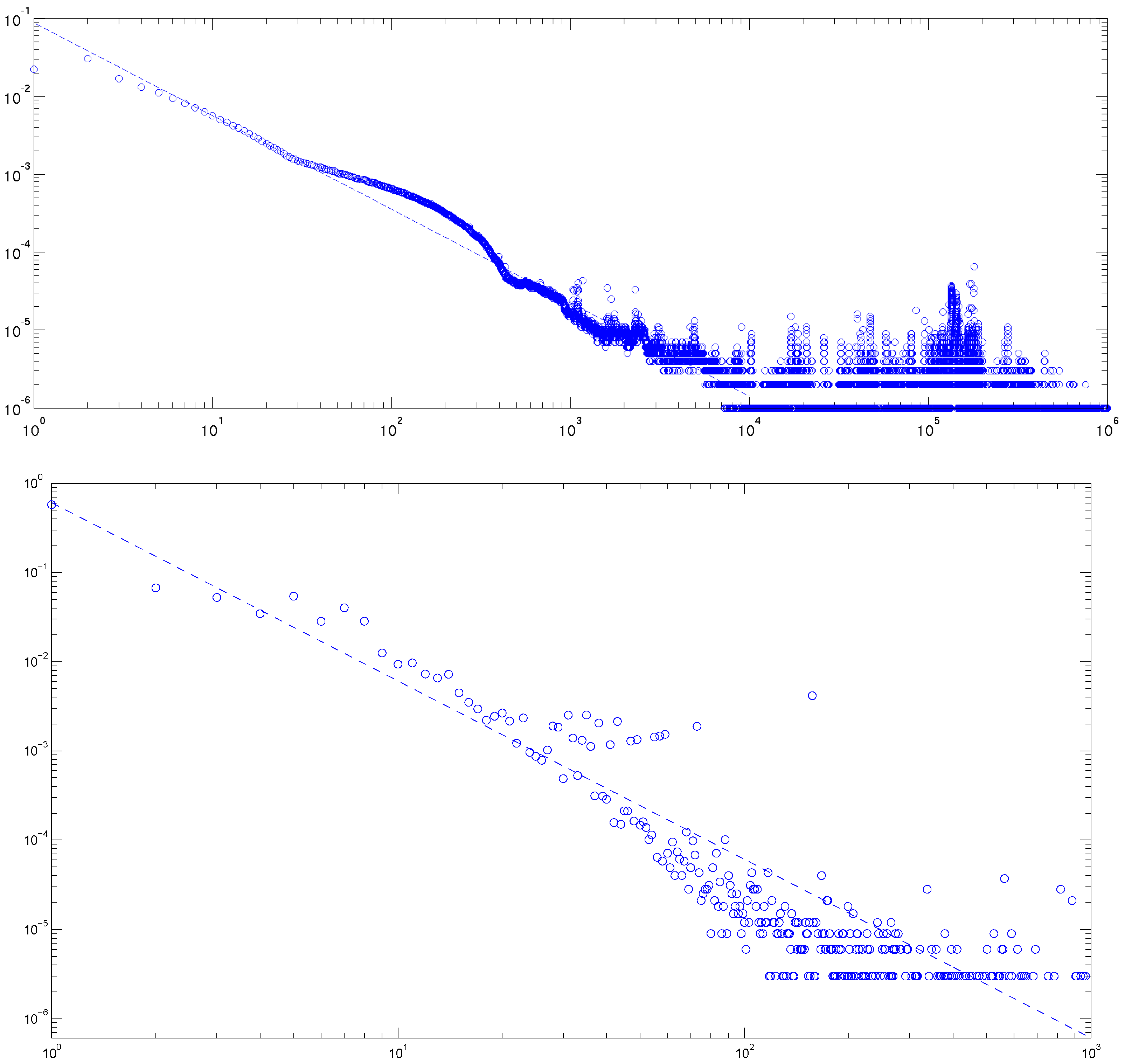
These properties induce that the gap between the index i of a page and the index j of one of its neighbours is typically small. The approach followed in this paper is based on ordering nodes based on the Breadth First Search (BFS) of the graph instead of the lexicographic order, while still retaining these features. In fact, Figure 1 (top) shows the corresponding distribution of the gaps between neighbours. This distribution follows a power law similar to the node degree distribution displayed in Figure 1 (bottom).
Figure 1.
The distribution of gaps between neighboring nodes (top) and (bottom) of node degrees in the dataset “in-2004” as gathered by Boldi and Vigna [3] using UbiCrawler [8].
The problem of graph compression has been approached by several authors over the years, perhaps beginning with the paper [9]. Among the most recent works, Feder and Motwani [10] looked at graph compression from the algorithmic standpoint, with the goal of carrying out algorithms on compressed versions of a graph. Among the earliest works specifically devoted to web graph compression one finds papers by Adler and Mitzenmacher [1], and Suel and Yuan [6]. For quite some time the best compression performance was that achieved by the WebGraph algorithm by Boldi and Vigna (BV in the following) [3], which uses two parameters to compress the Web Graph : the refer range W and the maximum reference count R. For each node BV represent a modified version of obtained from an adjacency list of another node () called the reference list (the value is called reference number). The representation is composed of a sequence of bits (copy list), which tells if a neighbour of is also a neighbour of , and the description of the extra nodes. Extra nodes are encoded using gaps that is, if the representation is . Table 1 reproduces an example from [3] of representation using copy list.

Table 1.
The Boldi and Vigna representation using copy lists [3].
| Node | Degree | Ref. N. | Copy List | Extra Nodes |
| … | … | … | … | … |
| 15 | 11 | 0 | 13, 15, 16, 17, 18, 19, 23, 24, 203 | |
| 16 | 10 | 1 | 011100110 | 22, 316, 317, 3041 |
| … | … | … | … | … |
The parameter R is the maximum size of a reference chain. In fact, BV do not consider all the nodes , with , to encode , but only those that produce a chain not longer than R. BV also developed ζ codes [11], a family of universal codes used to compress power law distributions with small exponent.
Claude and Navarro (CN) [4] proposed a modified version of Re-Pair [12] to compress the Web Graph. Re-Pair is an algorithm that builds a generative grammar for a string by hierarchically grouping frequent pairs into variables, frequent variable pairs into more variables and so on. Along these lines, CN essentially applies Re-Pair to the string that results from concatenation of the adjacency lists of the vertices. The data plots presented in [4] display that their method achieved a compression comparable to BV (at more than 4 bits per link) but the retrieval time of the neighbours of a node is faster.
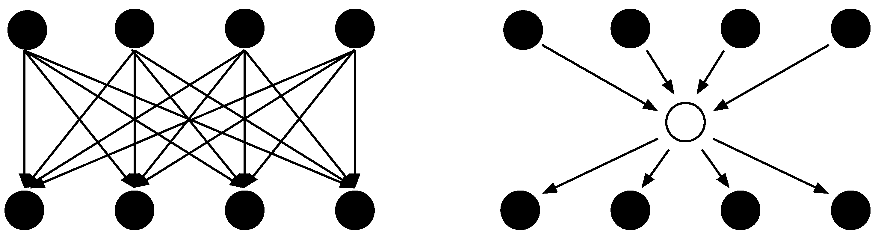
Buehrer and Chellapilla [7] (BC) proposed a compression based on a method presented in [10] by Feder and Motwani; They search for recurring dense bipartite graphs (communities) and for each occurrence found they generate a new node, called virtual node, that replaces the intra-links of the community (see Figure 2). In [13] Karande et al. showed that this method has competitive performances over well know algorithms including PageRank [14,15].
Figure 2.
The method by Buehrer and Chellapilla [7] compresses a complete bipartite graph (left) by introducing a virtual node (right).
Figure 2.
The method by Buehrer and Chellapilla [7] compresses a complete bipartite graph (left) by introducing a virtual node (right).
In [2], Asano et al. obtained better compression result than BV and BC but their technique does not permit a comparably fast access to the neighbours of a node. They compressed the intra-host links (that is, links between pages residing in the same host) by identifying through local indices six different types of blocks in the adjacency matrix, respectively dubbed: isolated 1-element, horizontal block, vertical block, L-shaped block, rectangular block, and diagonal block. Each block is represented by its first element, its type, and its size. The inter-host links are compressed by the same method used for the intra-host links, through resort to ad-hoc “new local indices” (refer to [2] for details).
3. Encoding by BFS
Our compression method is based on the topological structure of the Web Graph rather than on the underlying URLs. Instead of assigning indices to nodes based on the lexicographical ordering of their URLs, we perform a breadth-first traversal of G and index each node according to the order in which it is expanded. We refer to this process, and the compression it induces, as Phase 1. Following this, we compress in Phase 2 all of the remaining links.
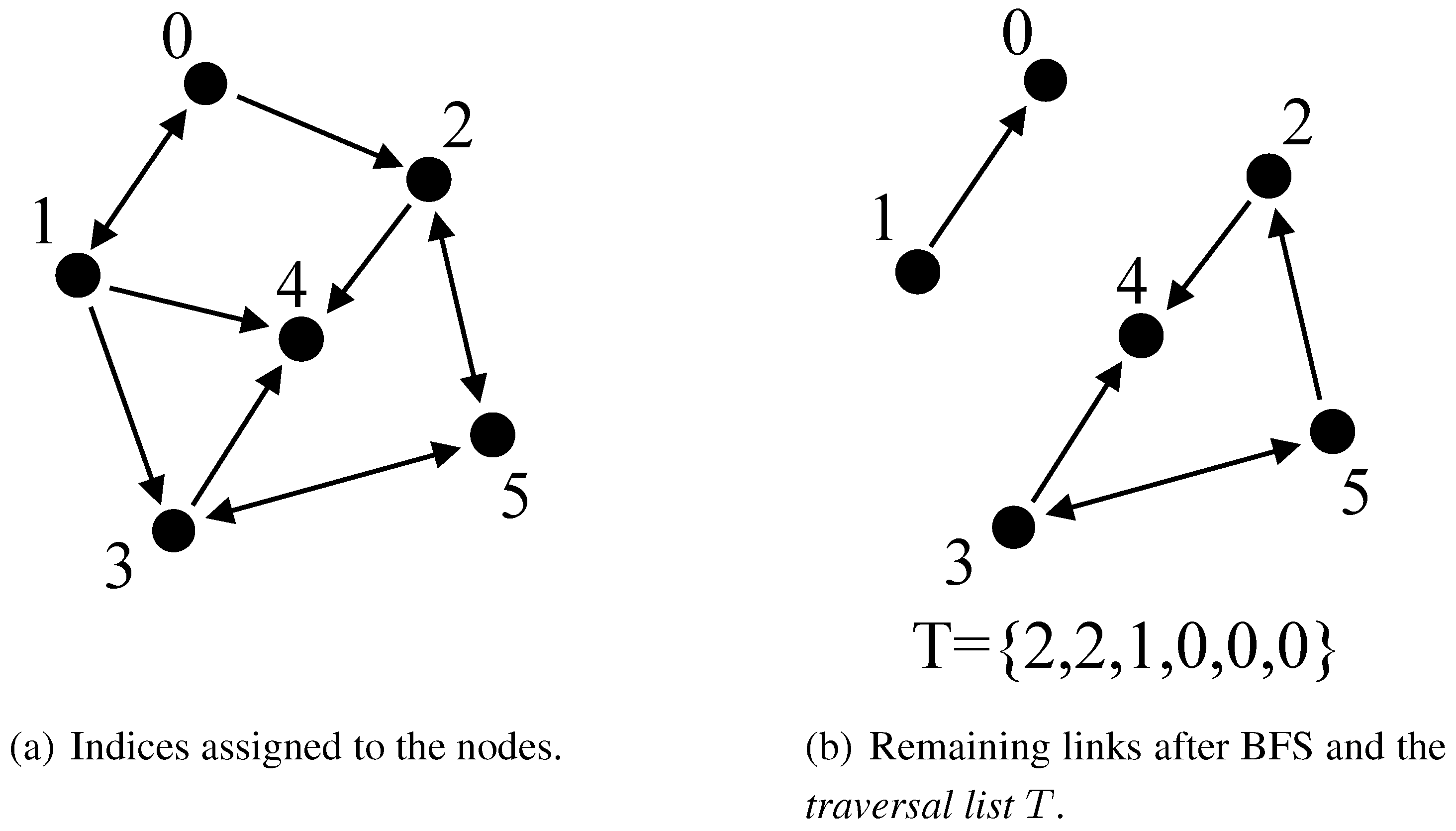
During the traversal of Phase 1, when expanding a node , we assign consecutive integer indices to its (not yet expanded) neighbours, and also store the value of . Once the traversal is over, all the links that belong to the breadth-first tree are encoded in the sequence , which we call the traversal list. In our experiments, the traversal allows to remove almost links from the graph. Figure 3 shows an example of Phase 1: the graph with the indices assigned to nodes is displayed in Figure 4(a), while Figure 4(b) shows the links remaining after the BFS and, below them, the traversal list. The compression ratio achieved by the present method is affected by the indices assignment of the BFS. In [16], Chierichetti et al. showed that finding an optimal assignment that minimizes is NP-hard.
Figure 3.
Illustrating Phase 1.
We now separately compress consecutive chunks of l nodes, where l is a prudently chosen value for what we call the compression level. Each compressed chunk is prefixed with the items of the traversal list that pertain to the nodes in the chunk: that is, assuming that the chunk C consists of the nodes , …, , then the compressed representation of C is prefixed by the sequence .
In Phase 2, we encode the adjacency list of each node in a chunk C in increasing order. Each encoding consists of the integer gap between adjacent elements in the list and a type indicator chosen in the set , β, χ, needed in decoding. With denoting the jth element in , we distinguish three main cases as follows.
- : the code is the string
- : the code is the string
- : this splits in two subcases, namely,
- (a)
- if then the code is the string
- (b)
- otherwise the code is the string
The types α and ϕ encode the gap with respect to the previous element in the list (), while β and χ are given with respect to the element in the same position of the adjacency list of the previous node ().
When does not exist it is replaced by , where k ( and ) is the closest index to i for which the degree of is not smaller than j, or by a ϕ-type code in the event that even such a node does not exist. In the following, we will refer to an encoding by its type. Table 3 displays the encoding that results under these conventions for the adjacency list of Table 2.
| Node | Degree | Links | ||||||||
| … | … | … | ||||||||
| i | 8 | 13 | 15 | 16 | 17 | 20 | 21 | 23 | 24 | |
| 9 | 13 | 15 | 16 | 17 | 19 | 20 | 25 | 31 | 32 | |
| 0 | ||||||||||
| 2 | 15 | 16 | ||||||||
| … | … | … | ||||||||
Table 3.
Encoding of the adjacency list of Table 2.
| Node | Degree | Links | ||||||||
| … | … | … | ||||||||
| i | 8 | ϕ 13 | ϕ 1 | ϕ 0 | ϕ 0 | ϕ 2 | ϕ 0 | ϕ 1 | ϕ 0 | |
| 9 | β 0 | β 0 | β 0 | β 0 | χ 0 | α 0 | β 2 | ϕ 5 | ϕ 0 | |
| 0 | ||||||||||
| 2 | β 2 | α 0 | ||||||||
| … | … | … | ||||||||
As mentioned, our encoding achieves that two nodes connected by a link are likely to be assigned close index values. Moreover, since two adjacent nodes in the Web Graph typically share many neighbors then the adjacency lists will feature similar consecutive lines. This leads to the emergence of four types of “redundancies” the exploitation of which is described, with the help of Table 4, as follows.
- A run of identical lines is encoded by assigning a multiplier to the first line in the sequence;
- Since there are intervals of constant node degrees (such as, for example, the block formed by two consecutive “9” in the table) then the degrees of consecutive nodes are gap-encoded;
- Whenever for some suitably fixed there is a sequence of at least identical elements (such as the block of ’s in the table), then this sequence is run-length encoded;
- Finally, a box of identical rows (such as the biggest block in the table) exceeding a pre-set threshold size is run-length encoded.
| Degree | Links | |||||||||
| … | … | |||||||||
| 0 | ||||||||||
| 9 | β 7 | ϕ 1 | ϕ 1 | ϕ 1 | ϕ 0 | ϕ 1 | ϕ 1 | ϕ 1 | ϕ 1 | |
| 9 | β 0 | β 1 | β 0 | β 0 | β 0 | β 0 | β 0 | β 0 | β 2 | |
| 10 | β 0 | β 1 | β 0 | β 0 | β 0 | β 0 | β 0 | β 0 | β 1 | ϕ 903 |
| 10 | β 0 | β 1 | β 0 | β 0 | β 0 | β 0 | β 0 | β 0 | β 223 | ϕ 900 |
| 10 | β 0 | β 1 | β 0 | β 0 | β 0 | β 0 | β 0 | β 0 | β 1 | α 0 |
| 10 | β 0 | β 1 | β 0 | β 0 | β 0 | β 0 | β 0 | β 0 | β 1 | β 0 |
| 10 | β 0 | β 1 | β 0 | β 0 | β 0 | β 0 | β 0 | β 0 | β 1 | β 0 |
| 10 | β 0 | β 1 | β 0 | β 0 | β 0 | β 0 | β 0 | β 0 | β 1 | β 0 |
| 10 | β 0 | β 1 | β 0 | β 0 | β 0 | β 0 | β 0 | β 0 | β 1 | β 0 |
| 10 | β 0 | β 1 | β 0 | β 0 | β 0 | β 0 | β 0 | β 0 | α 76 | α 232 |
| 9 | β 0 | β 1 | β 0 | β 0 | β 0 | β 0 | β 0 | β 0 | β 0 | |
| … | … | |||||||||
We exploit the redundancies according to the order in which they are listed above, and if there is more than one box beginning at the same entry we choose the largest one.
In order to signal the third or fourth redundancy to the decoder we introduce a special character Σ, to be followed by a flag denoting whether the redundancy starting with this element is of type 3 ( = 2), 4 ( = 3), or both ( = 1).
For the second redundancy in our example we write “ϕΣ 2 1 1”, where ϕ identifies a ϕ-type encoding, 2 is the value of , the first 1 is the gap, and the second 1 is the number of times that the element appears minus (2 in this example).
To represent the third redundancy both width and height of the box need encoding, thus in our example we can write “β Σ 3 0 7 5”, where β is the code type, 3 is the value of , 0 is the gap, 7 is the width minus 1, and 5 is the height minus 2.
When a third and fourth type redundancy originate at the same entry, both are encoded in the format “type Σ 1 gap l ”, where the 1 is the , l is the number of identical elements on the same line starting from this element, and w and h are, respectively, the width and the height of the box.
Table 5 shows the encoding resulting from this treatment.
| Lines | Degree | Links | |||
| … | … | … | |||
| 0 | 0 | ||||
| 0 | 9 | β 7 | ϕΣ 2 1 1 | ϕ 0 | ϕΣ 2 1 2 |
| 0 | 0 | βΣ 3 0 7 5 | β 1 | βΣ 2 0 4 | β 2 |
| 0 | 1 | β 1 | ϕ 903 | ||
| 0 | 0 | β 223 | ϕ 900 | ||
| 0 | 0 | β 1 | α 0 | ||
| 3 | 0 | β 1 | β 0 | ||
| 0 | 0 | α 76 | α 232 | ||
| 0 | -1 | β 0 | |||
| … | … | … | |||
We observe that we do not need to explicitly write ϕ characters, which are implicit in , a condition easily testable at the decoder. We encode the characters α, β and χ as well as by Huffman-code. Gaps, the special character Σ (Σ is an integer that does not appear as a gap) and other integers are encoded using the ad-hoc π-code described in the next section. When a gap g could be negative (as with degrees), then we encode if g is positive, and when .
4. A Universal Code
In this section we briefly introduce π-codes, a new family of universal codes for the integers. This family is better suited than the δ- and ζ- codes [11,17] to the cases of an entropy characterized by a power law distribution with an exponent close to 1.
| n | δ | ||||
| 1 | 1 | 11 | 111 | 1111 | 1 |
| 2 | 010 | 100 | 1100 | 11100 | 0100 |
| 3 | 011 | 101 | 1101 | 11101 | 0101 |
| 4 | 00100 | 01100 | 10100 | 110100 | 01100 |
| 5 | 00101 | 01101 | 10101 | 110101 | 01101 |
| 6 | 00110 | 01110 | 10110 | 110110 | 01110 |
| 7 | 00111 | 01111 | 10111 | 110111 | 01111 |
| 8 | 0001000 | 010000 | 100000 | 1100000 | 00100000 |
Let n be a positive integer, b its binary representation and . Having fixed a positive integer k, we represent n using bits. Specifically, say ( and ), then the -encoding of n is produced by writing the unary representation of l, which is followed by the k bits needed to encode c, and finally by the rightmost bits of b.
For instance, the -encoding of 21 is 01 11 0101: since the binary representation b of 21 is 10101 and we can write , then the prefix of the encoding is the unary representation of , the 2 bits that follow indicate the value of and the suffix is formed by the least significant digits of b. In the following we use the approximation described in [17], where is the entropy of a distribution with probability P. The expected length for n is:
A code is universal [17] if the expected codeword length is bounded in the interval . Each π-code is universal according to:
In the context of Web Graph compression we use a modified version of π-codes in which 0 is encoded by 1 and any other positive integer n is encoded with a 0 followed by the π-code of n.
5. Experiments
Table 8 reports sizes expressed in bits per link of our compressed graphs. We used datasets (Datasets and WebGraph can be downloaded from http://webgraph.dsi.unimi.it/) collected by Boldi and Vigna [3] (salient statistics in Table 7). Many of these datasets were gathered using UbiCrawler [8] by different laboratories.
With a compression level the present method yielded consistently better results than BV [3], BC [7] and Asano et al. [2]. The BV highest compression scores () are comparable to those we obtain at level 8, while those for general usage () are comparable to our level 4. Table 8 displays also the results of the BV method using an ordering of the URLs induced by the BFS. This indicates that BV does not take advantage.
| Nodes | Links | Avg Degree | Max Degree | |
| cnr-2000 | 325,557 | 3,216,152 | 9.88 | 2716 |
| in-2004 | 1,382,908 | 16,917,053 | 12.23 | 7753 |
| eu-2005 | 862,664 | 19,235,140 | 22.30 | 6985 |
| indochina-2004 | 7,414,866 | 194,109,311 | 26.18 | 6985 |
| uk-2002 | 18,520,487 | 298,113,762 | 16.10 | 2450 |
| arabic-2005 | 22,744,080 | 639,999,458 | 28.14 | 9905 |
| BV [3] | BC [7] | Asano et al. [2] | This Paper | ||||||
| BFS | BFS | ||||||||
| cnr-2000 | 3.92 | 3.56 | 3.23 | 2.84 | - | 1.99 | 1.87 | 2.64 | 3.33 |
| in-2004 | 3.05 | 2.82 | 2.35 | 2.17 | - | 1.71 | 1.43 | 2.19 | 2.85 |
| eu-2005 | 4.83 | 5.17 | 4.05 | 4.38 | 2.90 | 2.78 | 2.71 | 3.48 | 4.20 |
| indochina-2004 | 2.03 | 2.06 | 1.46 | 1.47 | - | - | 1.00 | 1.57 | 2.09 |
| uk-2002 | 3.28 | 3.00 | 2.46 | 2.22 | 1.95 | - | 1.83 | 2.62 | 3.33 |
| arabic-2005 | 2.58 | 2.81 | 1.87 | 1.99 | 1.81 | - | 1.65 | 2.30 | 2.85 |
To randomly access the graph we need to store the offset of the first element of each chunk, but the results shown here do not account for these offsets. In fact, we do need offsets. BV use in their tests, which are slowed down by about 50% setting . In BC an offset per node is required. Asano et al. do not provide information about offsets. In order to recover the links of the BFS tree, we also need to store for the first node u of each chunk the smallest index of a node v such that belongs to the BFS tree. In total, this charges an extra bits per node, where b bits are charged by the offset and k by the index of the node. With r the bits per link and d the average degree of a graph, b requires at most bits and k at most bits by Elias-Fano encoding [18, 19]. Using the same encoding, BC and BV require bits per node to represent any offset. Since , then we need less memory to store this information. Currently, in our implementation we use 64 bits per node.
Table 9 displays average times to retrieve adjacencies of random nodes. The tests run on an Intel Core 2 Duo T7300 2.00 GHz with 2 GB main memory and 4 MB L2-Cache under Linux 2.6.27. For the tests, we use the original Java implementation of BV (running under java version 1.6.0) and a C implementation of our method compiled with gcc (version 4.3.2 with -O3 option). The performance of Java and C are comparable [20], but we turned off the garbage collector anyway to speed-up. Table 9 shows that the BV high compression mode is slower than our method, while the BV general usage version () performs with comparable speed. However, settling for our method becomes faster.
| BV [3] | This Paper | |||
| cnr-2000 | 1.66 μs | 1.22 ms | 1.40 μs | 0.95 μs |
| in-2004 | 1.89 μs | 0.65 ms | 1.55 μs | 1.13 μs |
| eu-2005 | 2.58 μs | 2.35 ms | 3.16 μs | 2.09 μs |
| indochina-2004 | 2.31 μs | 0.93 ms | 2.42 μs | 1.72 μs |
| uk-2002 | 2.35 μs | 0.20 ms | 2.16 μs | 1.52 μs |
| arabic-2005 | 2.80 μs | 1.15 ms | 3.09 μs | 2.11 μs |
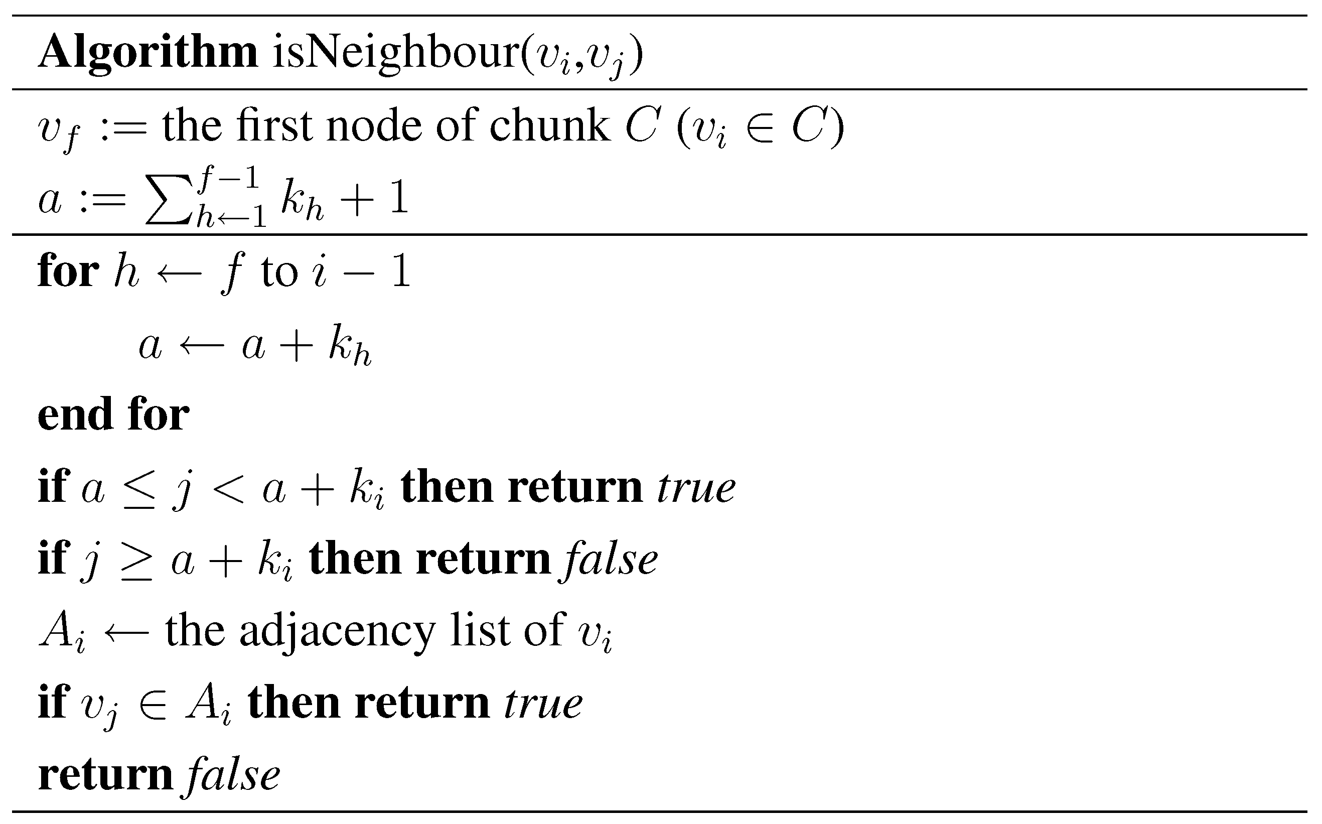
Figure 4.
Algorithm to check if the directed link (, ) exists.

| This Paper | ||
| cnr-2000 | 0.86 μs | 0.59 μs |
| in-2004 | 0.95 μs | 0.70 μs |
| eu-2005 | 1.73 μs | 1.20 μs |
| indochina-2004 | 1.55 μs | 1.11 μs |
| uk-2002 | 1.30 μs | 0.95 μs |
| arabic-2005 | 1.81 μs | 1.23 μs |
By virtue of the underlying BFS, we can implement a fast query to check whether or not a link exists. In fact, we know that a node has links that belong to the BFS tree, say, to , …, . We also know that does not have any link with a node where , so we need to generate the adjacency list of only if . Figure 4 displays the pseudocode of this query. Table 10 shows average times to test the connectivity of pairs of random nodes. The average time is less than of the retrieval time.
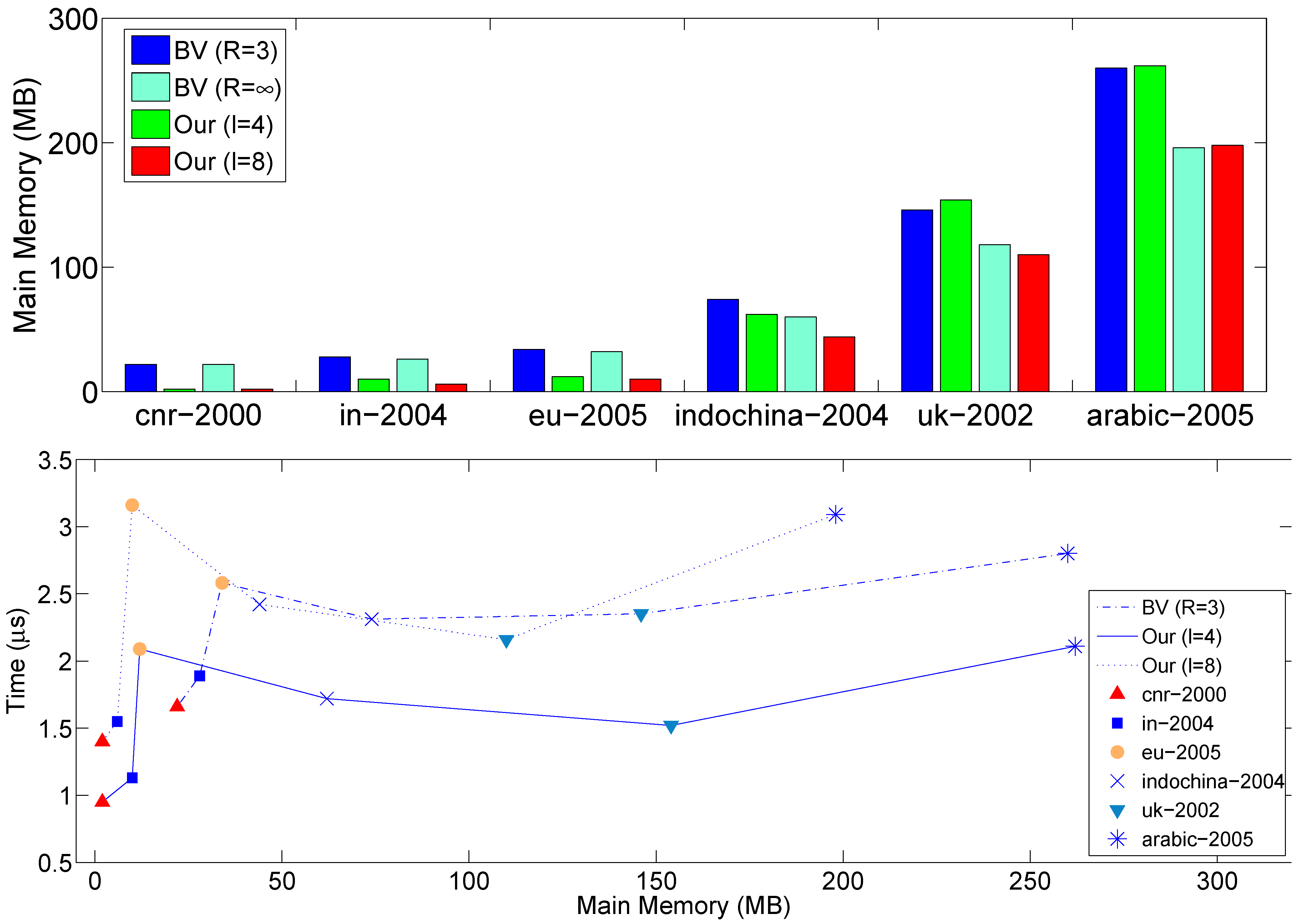
Finally, Figure 5 presents the actual main memory (top) respectively required by BV and our method, and the space-time tradeoff (bottom). As said, we do not compress the offsets. The space requirement of our compression level 8 is 80% of BV at .
Figure 5.
Main memory usage (top) by BV and the present method and the space-time tradeoff (bottom).
Figure 5.
Main memory usage (top) by BV and the present method and the space-time tradeoff (bottom).

6. Conclusion
We have proposed a new way to compress the Web Graph and other graphs of comparable structure. In fact, we assume no a priori knowledge of the graph, and in contrast with previous works based on lexicographic ordering of URLs we use a traversal to order nodes. The size of the compressed files is smaller of that of Asano et al. [2], considered the current state of the art. The average retrieval time is comparable to that of BV [3]. We also introduced a fast query to check whether two nodes are connected, without need to generate an entire adjacency list. Future work shall extend the set of primitive queries for compressed graphs.
References and Notes
- Adler, M.; Mitzenmacher, M. Towards compressing web graphs. In Proceedings of the IEEE Data Compression Conference, Snowbird, Utah, USA, March 27-29, 2001; pp. 203–212.
- Asano, Y.; Miyawaki, Y.; Nishizeki, T. Efficient compression of web graphs. In Proceedings of the 14th annual international conference on Computing and Combinatorics, Dalian, China, June 27 - 29, 2008; Springer-Verlag: Berlin, Heidelberg, Germany, 2008; pp. 1–11. [Google Scholar]
- Boldi, P.; Vigna, S. The web graph framework I: Compression techniques. In Proceedings of the Thirteenth International World Wide Web Conference, New York, NY, USA, 2004; ACM Press: Manhattan, USA, 2004; pp. 595–601. [Google Scholar]
- Claude, F.; Navarro, G. A fast and compact web graph representation. In Proceedings of 14th International Symposium on String Processing and Information Retrieval, Santiago, Chile, October 29-31, 2007; pp. 105–116.
- Randall, K.H.; Stata, R.; Wiener, J.L.; Wickremesinghe, R.G. The link database: fast access to graphs of the web. In Proceedings of the Data Compression Conference (DCC ’02), Snowbird, UT, USA, April 2-4, 2002; IEEE Computer Society: Washington, DC, USA, 2002; p. 122. [Google Scholar]
- Suel, T.; Yuan, J. Compressing the graph structure of the web. In Proceedings of the IEEE Data Compression Conference, Snowbird, Utah, USA, March 27-29, 2001; pp. 213–222.
- Buehrer, G.; Chellapilla, K. A scalable pattern mining approach to web graph compression with communities. In Proceedings of the international conference on Web search and web data mining, Palo Alto, CA, USA, February 11-12, 2008; ACM: New York, NY, USA, 2008; pp. 95–106. [Google Scholar]
- Boldi, P.; Codenotti, B.; Santini, M.; Vigna, S. UbiCrawler: a scalable fully distributed web crawler. Software: Pract. Exp. 2004, 34, 711–726. [Google Scholar] [CrossRef]
- Turan, G. On the succinct representation of graphs. Discrete Appl. Math. 1984, 8, 289–294. [Google Scholar] [CrossRef]
- Feder, T.; Motwani, R. Clique partitions, graph compression and speeding-up algorithms. J. Comput. Syst. Sci. 1995, 51, 261–272. [Google Scholar] [CrossRef]
- Boldi, P.; Vigna, S. Codes for the world wide web. Internet Math. 2005, 2, 407–429. [Google Scholar] [CrossRef]
- Larsson, N.J.; Moffat, A. Offline dictionary-based compression. IEEE 2000, 88, 1722–1732. [Google Scholar] [CrossRef]
- Karande, C.; Chellapilla, K.; Andersen, R. Speeding up algorithms on compressed web graphs. In Proceedings of the Second ACM International Conference on Web Search and Data Mining, Barcelona, Spain, February 9-12, 2009; ACM: New York, NY, USA, 2009; pp. 272–281. [Google Scholar]
- Brin, S.; Page, L. The anatomy of a large-scale hypertextual web search engine. Comput. Netw. ISDN Syst. 1998, 30, 107–117. [Google Scholar] [CrossRef]
- Page, L.; Brin, S.; Motwani, R.; Winograd, T. The pagerank citation ranking: bringing order to the web; Technical Report 1999-66; Stanford InfoLab, 1999; Previous number = SIDL-WP-1999-0120. [Google Scholar]
- Chierichetti, F.; Kumar, R.; Lattanzi, S.; Mitzenmacher, M.; Panconesi, A.; Raghavan, P. On compressing social networks. In Proceedings of the 15th ACM SIGKDD international conference on Knowledge discovery and data mining, San Diego, CA, USA, August 15-18, 1999; ACM: New York, NY, USA, 2009; pp. 219–228. [Google Scholar]
- Elias, P. Universal codeword sets and representations of the integers. IEEE Trans. Inf. Theory 1975, 21, 194–203. [Google Scholar] [CrossRef]
- Elias, P. Efficient storage and retrieval by content and address of static files. J. ACM 1974, 21, 246–260. [Google Scholar] [CrossRef]
- Fano, R.M. Project MAC. Computer Structures Group Memorandum 61. On the number of bits required to implement an associative memory; Massachusetts Institute of Technology: Cambridge, MA, USA, 1971. [Google Scholar]
- Lewis, J.; Neumann, U. Performance of java versus C++; Computer Graphics and Immersive Technology Lab, University of Southern California: Los Angeles, CA, USA, 2003. [Google Scholar]
© 2009 by the authors. Licensee Molecular Diversity Preservation International, Basel, Switzerland. This article is an open-access article distributed under the terms and conditions of the Creative Commons Attribution license ( http://creativecommons.org/licenses/by/3.0/).
Share and Cite
MDPI and ACS Style
Apostolico, A.; Drovandi, G. Graph Compression by BFS. Algorithms 2009, 2, 1031-1044. https://doi.org/10.3390/a2031031
AMA Style
Apostolico A, Drovandi G. Graph Compression by BFS. Algorithms. 2009; 2(3):1031-1044. https://doi.org/10.3390/a2031031
Chicago/Turabian StyleApostolico, Alberto, and Guido Drovandi. 2009. "Graph Compression by BFS" Algorithms 2, no. 3: 1031-1044. https://doi.org/10.3390/a2031031