Classification of Sperm Whale Clicks (Physeter Macrocephalus) with Gaussian-Kernel-Based Networks

Abstract

With the aim of classifying sperm whales, this report compares two methods that can use Gaussian functions, a radial basis function network, and support vector machines which were trained with two different approaches known as C-SVM and ν-SVM. The methods were tested on data recordings from seven different male sperm whales, six containing single click trains and the seventh containing a complete dive. Both types of classifiers could distinguish between the clicks of the seven different whales, but the SVM seemed to have better generalisation towards unknown data, at the cost of needing more information and slower performance.

1. Introduction

Sperm whales (Physeter macrocephalus), when living in a social community, often forage in small groups. During their feeding dive, which may be to depths up to 2 kilometres [1], they start producing sonar signals fairly soon after the start of a dive and generally continue until the ascent back to the surface. Usually one click per second is produced on average, but at times this frequency is increased (presumably when they have found prey) and up to fifty signals per second may be produced [2]. This sequence of very rapid clicks is called a creak, and the period from the start of a click sequence to a creak, or a prolonged moment of silence, is called a click train. The recording of these diving groups results in a mixture of signals, and the manual assignment of a click from a click train to the animal that produced it is often a difficult and arduous task. To this end, we want to build an automated method that can distinguish between clicks from different animals using primarily characteristic information in the clicks themselves. This could then be combined with, for example, time delays of arrival at the hydrophones to reliably reconstruct the original click trains for the individual whales.

When recorded on axis, a click consist of a series of up to five pulses separated by a few milliseconds where the second pulse dominates strongly over the others. A relative difference of 40 dB in signal level can be encountered [3]. The clicks are broad band with energy in frequencies exceeding 30 kHz and a peak frequency around 12 kHz. However, when recording off axis, as is almost always the case in practice, the signal becomes distorted with strong attenuation of this second pulse. The click’s characteristics may change depending on the animal’s orientation and distance to the hydrophone, while the animal’s depth [4] and activities may play a role as well. A typical example of a low-pass filtered clicks is shown in Figure 1. Each image in this figure contains 10 consecutive clicks superimposed on each other. Synchronisation was done with a low frequency matched filter. It can be seen how the signal changes through the click train. Focusing on for example the area around sample 210, a new peak appears probably due to different time delays between the click’s pulses that can be caused by changes in the animal’s orientation with respect to the hydrophone. Research has shown [5] that dominant frequencies of off axis clicks for both male and female sperm whales can be found below 2,000 Hz. Since low frequencies are less influenced by orientation or distance, they are more suitable to be searched for constant characteristics.

Figure 1. Example clicks from one animal at different moments in the click train. Each image contains 10 consecutive superimposed clicks that were filtered below 3,000 Hz and normalised in energy. A pulse seems to be moving from left to right, especially visible around sample 210.

Figure 1. Example clicks from one animal at different moments in the click train. Each image contains 10 consecutive superimposed clicks that were filtered below 3,000 Hz and normalised in energy. A pulse seems to be moving from left to right, especially visible around sample 210.

An earlier attempt has been made to identify a whale based on modelling these dominant frequencies directly using a Gabor function [6]. The use of Gabor functions is interesting as it suggests that nature uses a signal optimised in a time-frequency sense, and they have been used successfully to describe dolphin sonar [7, 8]. However, it was found that the dominant frequencies were not stable enough to be used as an identifier for the entire duration of a dive. Similarly, in the same study, a simple linear classification method was not able to distinguish clearly between individuals in a small group of whales, and therefore this report looks at non-linear classifiers in the form of a neural network. Neural networks have been used in the past for marine mammal classification with some success [9, 10]. The distribution of the characteristics from the sperm whale clicks suggested the use of a Gaussian model, and therefore a radial basis function network (RBF) architecture was used in [11] to separate sperm whales. Here, we compare the performance of radial basis functions with support vector machines (SVM) [12, 13]. SVM use a similar network architecture, but follow a different underlying approach and are trained differently. Training of the SVM was done in the standard approach, known as C-SVM, and a second approach known as ν-SVM [14, 15]. An advantage of the latter method is that there is a more direct control on the number of support vectors used by the machine.

2. Data Acquisition, Preparation and Feature Selection

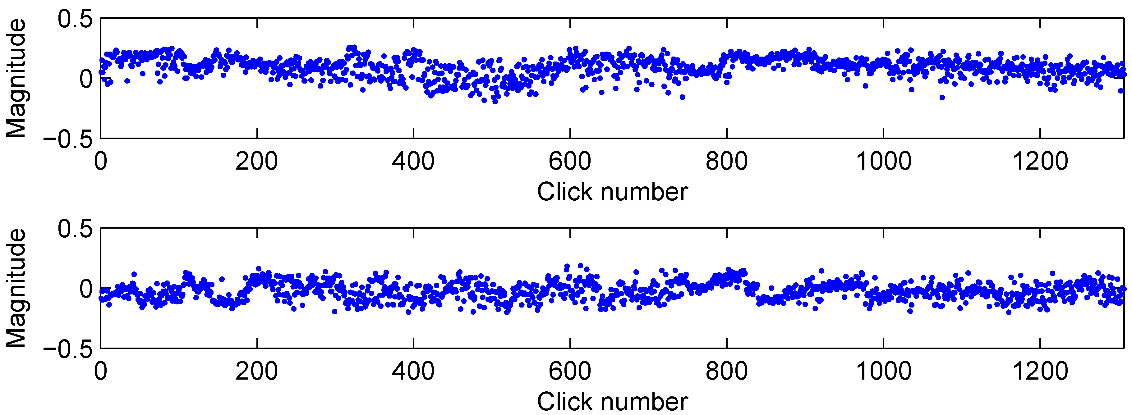
2.1. Data acquisition

The sperm whale data were collected from an inflatable boat during four field seasons spanning four to ten weeks each (from 1997 to 1999) at Kaikoura, New Zealand [16]. Recordings were made of solitary diving male sperm whales using an omni-directional hydrophone (Sonatech 8,178; frequency response 100 Hz to 30 kHz ± 5 dB) lowered to a depth of 20 m. This hydrophone was first connected to a fixed gain amplifier (flat response from 0 to 45 kHz) and then to one channel of a Sony TCD-D10PROII Digital Audio Tape recorder (frequency response 20 Hz to 22 kHz ± 1 dB with an anti-alias filter at 22 kHz). The recordings were digitized at 48 kHz and 16 bits. The use of data from solitary diving whales guarantees that no data from different animals were mixed, thus helping to obtain optimal results. The typical duration of the recorded click trains was around 2.5 mins. The 30 mins complete dive was a sequence of such click trains. The dive was divided in 10 data segments to ease data handling and manual analysis, but these did not exactly cover 10 click trains as the trains themselves are not always very well defined. A pause in the click production is sometimes too short to consider the continuation to be a new click train, but rather it can indicate that a few signals were not detected. Generally, a click train ends with a creak where it is assumed the animal is capturing a prey, but this is not always heard on a recording as the signal can be too weak.

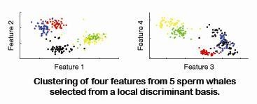
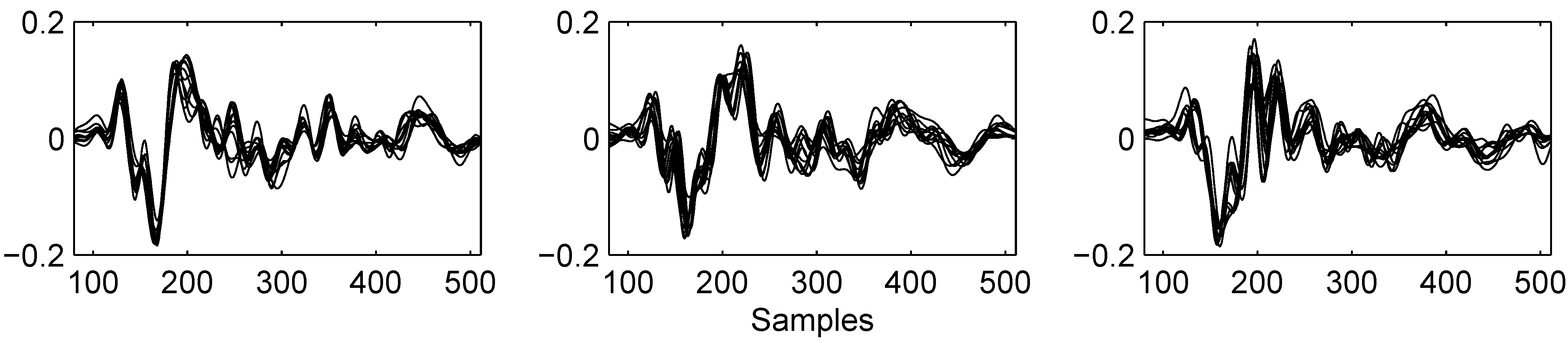
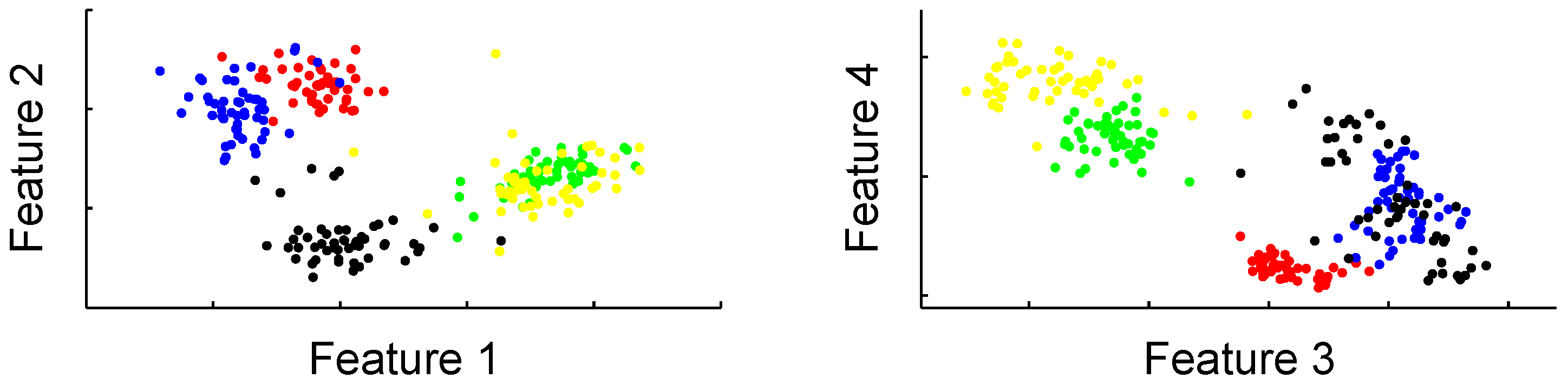
2.2. Data preparation and feature selection

In preparation for the classification algorithm, the clicks were manually detected, filtered for echoes, and checked for acceptable noise levels. These clicks were then denoised using a standard soft-thresholding algorithm, available in Wavelab [17], and synchronised using a matched filter on the low dominant frequency with a typical example click. Initially, the data were band-pass filtered between 100 and 20,000 Hz.

Data from seven different animals were available for this study, comprised of six single click trains and a complete dive. This dive was considered to be especially interesting as it allowed to see the performance of the algorithm, and validity of features, for the duration of an entire dive. Therefore, the dive was split up in two unequal parts. One click train early in the dive was separated and joined together with the other six available click trains used for training. The remainder of the dive was put in its own set and was only used to test the classifier, it was never used for training or parameter selection. This approach simulated the situation where a classifier would have to be trained with data at the start of a recording and allowed to assess its capacity to generalise to patterns much later in the dive sequence, that may have undergone changes as in Figure 1.

The seven click trains were used to train the classifiers. As the objective of the classification is that a classifier can be trained with only the start of a recording and then autonomously classify the remainder, only the first 50 clicks were used from the start of each click train, which corresponds to roughly 50 seconds. The other available patterns in the click trains were used for validation, but were never considered for training.

The features were selected using a local discriminant basis [18, 19] for the seven classes. The exact same procedure was followed as in [6]. First, each click in the training set was expressed in a wavelet packet table. Where the usual wavelet filter retains the high-pass wavelet coefficients and continues filtering the low-pass scale coefficients, the wavelet packet table filters both outputs again, creating a redundant library of bases that can be selected for reconstruction of the signal (a detailed discussion about the relationship between wavelets and filter banks can be found in [20]). With each pass through the wavelet filter the frequency band of the input signal is split in two, producing low and high frequency outputs. These outputs are stored and passed through the filter again. In this paper these recursive steps will be called the splitting level, e.g., at level 3 the signal has been passed through the filter twice. At a splitting level l there will be $2^{l-1}$ band limited signals, each with a bandwidth of $F_s/2^l$ with $F_s$ the sampling frequency. These signals will be called frequency bins (holding the energy of their respective frequency bands) and indexed with k. The coefficients inside each bin will be indexed by m. After the creation of the packet table, a basis is selected that emphasises the differences between the classes. This difference is measured with the help of a time-frequency energy map, defined as follows:

$${\Gamma }_c(j,k,m)=\sum _i^{N_c}{\left({\widehat{x}}_i^c(j,k,m)\right)}^2/\sum _i^{N_c}\left|\right|{\mathbf{x}}_i^c{\left|\right|}^2$$

(1)

where $(j,k,m)$ denotes the position in the packet table, at splitting level j, frequency band k and coefficient m within the bin; ${\widehat{x}}_i^c(j,k,m)$ denotes the wavelet coefficient of click sample i and class c at position $(j,k,m)$; ${\mathbf{x}}_i^c$ the click sample i of class c; $N_c$ the number of training samples in class c. This map basically sums the packet tables of the clicks within one class and allows the comparison of the energy in a specific bin $(j,k,·)$ between different classes. This discrepancy can be measured with the following function,

$$\begin{array}{ccc}\hfill \mathcal{D}(j,k,·)& =& \sum _m\sum _{p=1}^{C-1}\sum _{q=p+1}^C\mathcal{D}({\Gamma }_p(j,k,m),{\Gamma }_q(j,k,m))\hfill \end{array}$$

Here the difference between every pair of classes is measured through an additive discriminant function $\mathcal{D}$, for which we used the squared $l^2$-norm. A high value for $\mathcal{D}$ means that that specific bin may be able to separate at least 2 classes that lie far apart. The local basis can now be selected using the following rule, if the measure on a bin $\mathcal{D}(j,k,·)$, is higher than the sum of the measures over the two bins it splits into, $\mathcal{D}(j+1,2k,·)+\mathcal{D}(j+1,2k+1,·)$, then it is selected, otherwise it is split. After the local discriminant basis was created, we selected the 15 strongest coefficients, according to Fisher’s discriminant given by :

$$FD=\frac{{\sum }_c{\left({\overline{s}}_i^c-{\text{mean}}_c\left({\overline{s}}_i^c\right)\right)}^2}{{\sum }_c{\text{var}}_i\left(s_i^c\right)}$$

(2)

where s are coefficients taken from a specific entry in the discriminating basis, and both the bar and ${\text{var}}_i$ take the mean and variance over all samples $s_i$ in class c and ${\text{mean}}_c$ takes the mean over all classes. Essentially, this expression measures the distance between the class means and their common centre with respect to their widths, leading to high values when samples in a class lie tightly around their class centre.

The 15 strongest features found using the selection procedure described above are summarised in Table 1. It is apparent that the best features were found in the lowest frequencies, where a dominant frequency can be found. Another reason why this may happen is that higher frequencies seem to be more variable in time, as was shown in Figure 1. A shift of a high frequency component will also shift its corresponding energy in the wavelet filter bank. The discrete wavelet transform with a symmlet wavelet as was used for this report has a very slow roll-off. After the down sampling step, aliasing will appear in and propagate through the filter bank. Normally, the aliasing (and phase distortion) is repaired in the synthesis step. This behaviour is not a problem for classification as long as it is consistent. However, phase delays in higher frequencies for consecutive clicks that cause subsequent energy shifts in the wavelet coefficients will act as a source of noise. Therefore, after it was confirmed that there were no high frequency features of interest, the algorithm was focussed on the lowest frequencies using a fifth order Butterworth low-pass filter at 2,000 Hz. After filtering the clicks were down sampled to remove redundant information. When this classification approach is followed on other data sets, the discriminant features should probably always first be selected from the full bandwidth to ensure optimal classification.

Table 1. Selected wavelet packet coefficients for discrimination. The given index $(k,m)$ is the position m of the coefficient in frequency band k at the given split level. The splitting level starts at 1, which indicates the original signal, i.e. at level 5 the signal was filtered 4 times.

index	split	frq band (Hz)	power	index	split	frq band (Hz)	power
(1,2)	5	1 - 1,500	3.5	(1,1)	5	1 - 1,500	3.4
(1,3)	5	1 - 1,500	3.0	(1,4)	5	1 - 1,500	2.3
(2,11)	5	1,500 - 3,000	1.3	(1,31)	5	1 - 1,500	1.2
(1,9)	5	1 - 1,500	1.0	(1,21)	5	1 - 1,500	0.95
(1,10)	5	1 - 1,500	0.80	(2,8)	5	1,500 - 3,000	0.80
(1,13)	5	1 - 1,500	0.79	(1,18)	5	1 - 1,500	0.79
(1,14)	5	1 - 1,500	0.76	(1,22)	5	1 - 1,500	0.73
(1,16)	5	1 - 1,500	0.65			-

Table 1. Selected wavelet packet coefficients for discrimination. The given index $(k,m)$ is the position m of the coefficient in frequency band k at the given split level. The splitting level starts at 1, which indicates the original signal, i.e. at level 5 the signal was filtered 4 times.

index	split	frq band (Hz)	power	index	split	frq band (Hz)	power
(1,2)	5	1 - 1,500	3.5	(1,1)	5	1 - 1,500	3.4
(1,3)	5	1 - 1,500	3.0	(1,4)	5	1 - 1,500	2.3
(2,11)	5	1,500 - 3,000	1.3	(1,31)	5	1 - 1,500	1.2
(1,9)	5	1 - 1,500	1.0	(1,21)	5	1 - 1,500	0.95
(1,10)	5	1 - 1,500	0.80	(2,8)	5	1,500 - 3,000	0.80
(1,13)	5	1 - 1,500	0.79	(1,18)	5	1 - 1,500	0.79
(1,14)	5	1 - 1,500	0.76	(1,22)	5	1 - 1,500	0.73
(1,16)	5	1 - 1,500	0.65			-

All classifiers were trained using the characteristics of the first 50 clicks of the seven sets, reflecting the situation where the start of a recording is manually separated by an expert (or automatically when possible), and the remaining data would be processed automatically by the computer. The other clicks within the sets, and the eighth set, were then used for validation.

Figure 2. Scatter plots of the four most discriminating features for five animals. The combination of these four characteristics already shows possible separation of five animals. Moreover, the features show a strong clustering tendency that suggests the use of a Gaussian model.

Figure 2. Scatter plots of the four most discriminating features for five animals. The combination of these four characteristics already shows possible separation of five animals. Moreover, the features show a strong clustering tendency that suggests the use of a Gaussian model.

Figure 3. Variability in the two strongest features (first feature on top, second on bottom) from Table 1 during the dive.

Figure 3. Variability in the two strongest features (first feature on top, second on bottom) from Table 1 during the dive.

Figure 2 shows a combination of two graphics with the four strongest features, measured using Fisher’s power of discrimination with Equation (2), from five animals that allows some insight in the feature space. The combination of just these four features already shows some possibility of separating the animals. Three animals are already separated in the left figure, while two are completely mixed. Combination with the two other characteristics in the right figure allows these two to be separated as well. An important observation in these figures, and one that we used to design the classifier, was that the data showed a strong clustering tendency. This suggested the application of a RBF network which has a natural way of modelling these clusters in its hidden layer, or a SVM which does not model the clusters themselves but their borders. Another reason we decided to use RBF and SVM based classifiers is because these methods have a local response defined by the distance of a sample to the cluster centres or support vectors. This is different from, for example, multi-layer perceptron networks, where a node in the first layer will give the same response for all points on a specific hyperplane. Although, as a result, perceptron networks may have better generalisation in areas of the feature space that are poorly sampled, we preferred the local properties that allowed more accurate modelling of the feature space as it is presented in Figure 2. To have an idea about the variability of the features, Figure 3 shows the two strongest features during the whole dive. From this figure it can be suspected that 50 consecutive samples may not always be sufficient to characterise the variance of the feature.

3. Classification Description

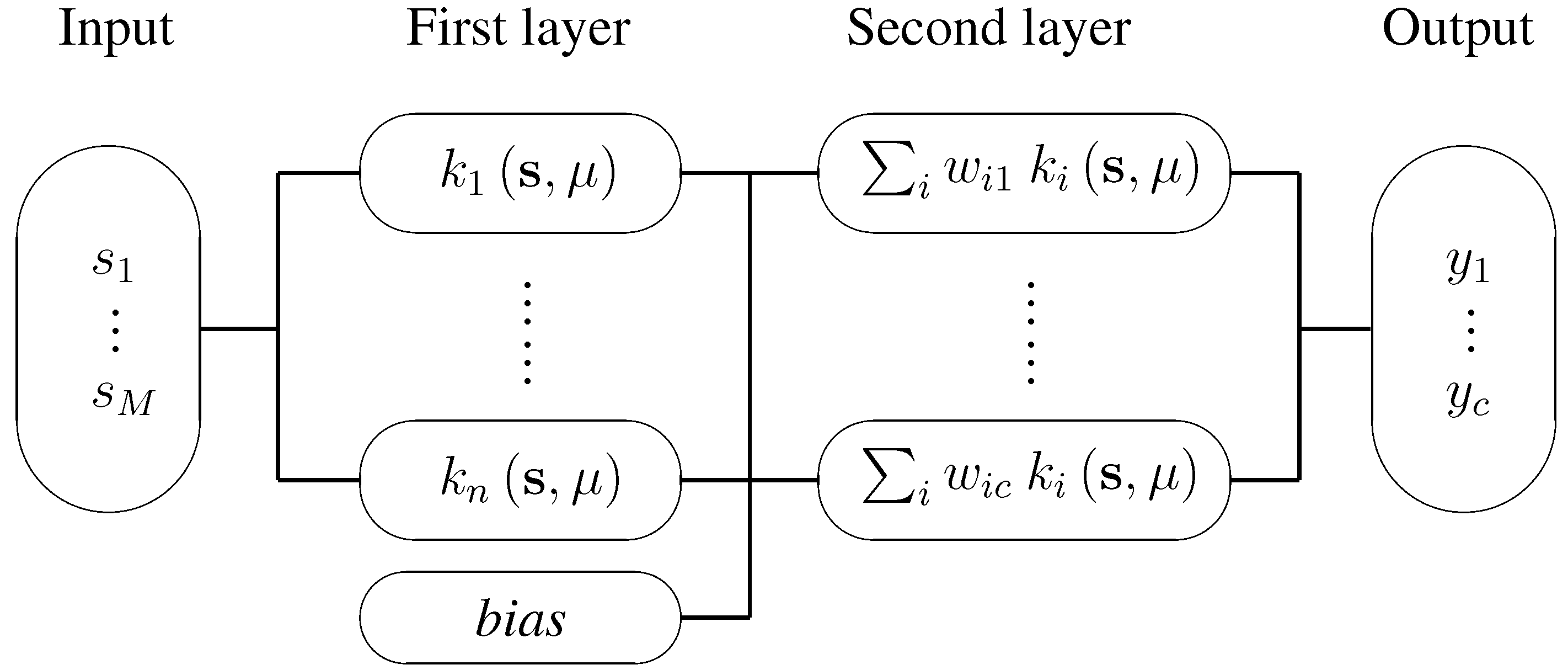
3.1. Radial basis function network

A detailed description about RBF networks can be found in [21]; its schematic is shown in Figure 4.

Figure 4. Schematic of an RBF-network. An M-dimensional sample $\mathbf{s}$ enters on the left, and is first run through the n hidden layer nodes where the distances between $\mathbf{s}$ and centres μ are evaluated through Gaussian functions $k_n(\mathbf{s},\mu )$. The outputs of the n Gaussian functions are then weighed with weights $w_{ij}$ and linearly combined in the second layer nodes (containing one node per class). Bias is usually represented with the help of a hidden layer node with a constant activation function, $k_0\equiv 1$. Each output layer then has a corresponding additional weight ($w_{0j}$) that accounts for the bias factor. Taking the output vector $\mathbf{y}$, the class of the sample $\mathbf{s}$ is computed by $arg{max}_i{y}_i$ .

Figure 4. Schematic of an RBF-network. An M-dimensional sample $\mathbf{s}$ enters on the left, and is first run through the n hidden layer nodes where the distances between $\mathbf{s}$ and centres μ are evaluated through Gaussian functions $k_n(\mathbf{s},\mu )$. The outputs of the n Gaussian functions are then weighed with weights $w_{ij}$ and linearly combined in the second layer nodes (containing one node per class). Bias is usually represented with the help of a hidden layer node with a constant activation function, $k_0\equiv 1$. Each output layer then has a corresponding additional weight ($w_{0j}$) that accounts for the bias factor. Taking the output vector $\mathbf{y}$, the class of the sample $\mathbf{s}$ is computed by $arg{max}_i{y}_i$ .

An important reason to consider this type of network was that its two layers can be trained separately, without the use of a non-linear optimisation routine. This allows the training stage to be executed fast and makes it suitable for real-time applications. For the hidden layer activation functions we chose the Gaussian function given by

$$k(\mathbf{s},\mu )=exp(-\frac{\left|\right|\mathbf{s}-{\mu \left|\right|}^2}{2{\sigma }^2})$$

(3)

where $\mathbf{s}$ is the input feature vector, μ controls the function’s centre, and σ its width. This layer was trained using a clustering algorithm, placing centres on top of dense locations in the data. One clustering algorithm that is used often is k-means [22], but this has the drawback that the number of clusters k has to be given in advance. There are various clustering methods that can search for an optimal (according to some defined statistic) number of clusters. One such method is described in [23], and we used a slightly adapted version. Initially, the clustering process starts with two clusters, splitting the data with k-means. A cluster was accepted and removed from the feature space when its projection in the direction of its principal component resembled a normal distribution, where normality was measured using the Anderson-Darling statistic [24, 25]. The value for k was then adjusted for the removed clusters and increased by one. The remaining clusters were combined and clustered again. This process was repeated until all clusters were accepted. To prevent random outcomes, k-means was always initialised by placing an additional centre in a cluster on the feature vector furthest away from the data’s centre [26]. In order to take advantage of class information in the clustering process, the clustering was done on the individual classes, instead of on all the data as a whole.

Once the first layer has been defined by the clusters, training of the second layer is trivial; the number of nodes was set to the number of classes, using binary encoding for the targets (e.g., a sample from class 1 has target ${\left[100\right]}^t$, and a sample from class 3 has target ${\left[001\right]}^t$). Calculation of the weights, using a sum-of-squares error function, is then a fast linear process [21].

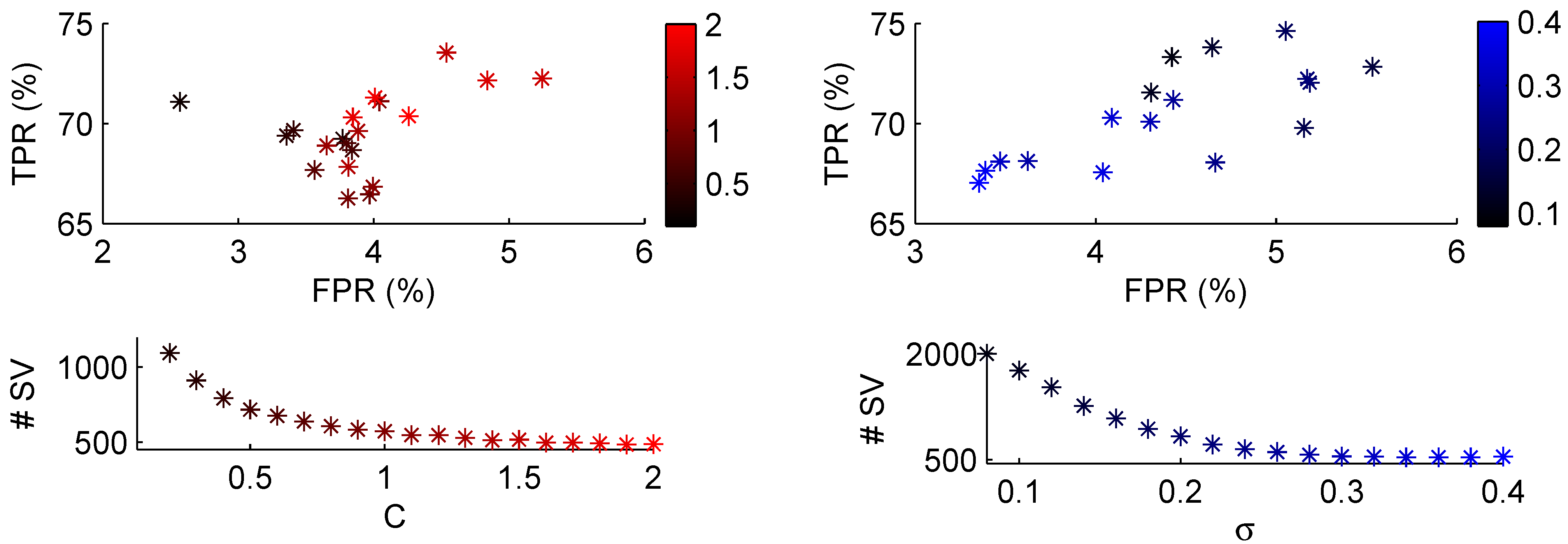
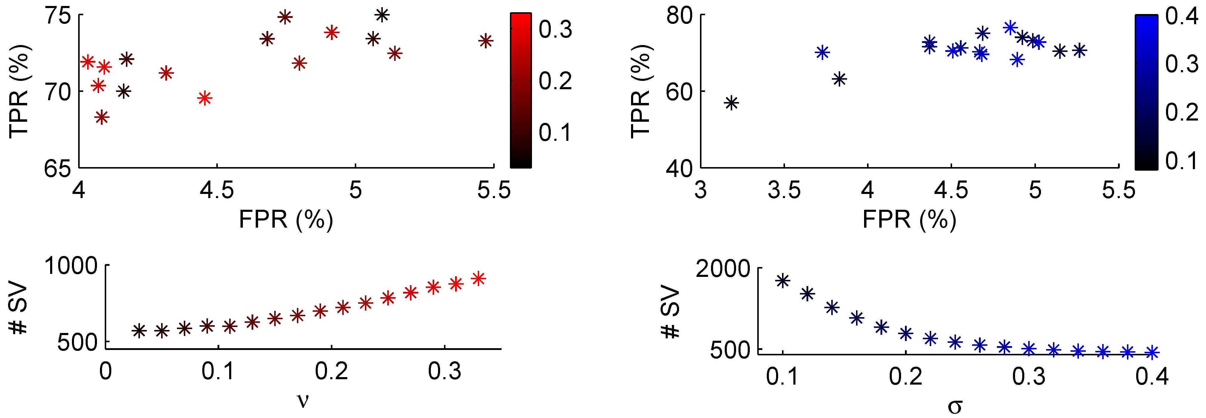
3.2. Support vector machine classification

Another popular network model that uses Gaussian functions are support vector machines (SVM). SVM generally solve the two class problem with a network structure that is similar to the RBF structure in Figure 4. Since there are only two classes, SVM only have one output. The main difference between the two networks relies on the underlying approach and in the way they are trained. Where the RBF network places Gaussian kernels on the cluster centres formed by the features in the feature space, the SVM network places the Gaussian kernels on those samples that define the boundary between two classes. These points are found by creating a separating hyperplane inside a higher dimensional feature space. A reason to consider SVM is that they tend to show strong generalisation performance [22]. In the case of SVM, the interpretation of the first layer is that it projects the data to a feature space where the two classes can be separated by a hyperplane. The position of the hyperplane is decided by those points that lie within a certain margin between the two classes (the support vectors). The projected feature space is allowed (or preferred) to have a higher dimension, as there is no penalty in the form of computational drawbacks or the ’curse of dimensionality’ since the actual mapping is never performed. All necessary calculations in the projected feature space are evaluated through inner products, which can be done with a kernel function. In our case this was the Gaussian function (3) that was also used for the RBF network.

The training stage for SVM both defines the number of nodes in the hidden layer and calculates the output layer weights at the same time. There several approaches to train the network in the case of non-separable classes. First we looked at C-SVM, which aims at solving the following optimisation problem [27]:

$$\underset{\mathbf{w},\xi ,b}{\text{min}}{\left|\right|\mathbf{w}\left|\right|}^2+C\sum _{i=1}^N{\xi }_i$$

(4)

under the constraint that the training data should classify correctly, and where $\mathbf{w}$ is the direction of the normal vector on the separating plane, N the number of samples, ξ are the slack vectors which are non-zero for the samples that lie within the margin, and C is the pre-defined penalty on these points. This problem has a straightforward optimal solution ${\mathbf{w}}_o$ using Lagrange multipliers [27], expressed as follows

$${\mathbf{w}}_o=\sum _{i=1}^N{\alpha }_i{t}_i\varphi \left({\mathbf{s}}_i\right)$$

(5)

where $t_i$ are the targets of mapped inputs ${\mathbf{s}}_i$. Only a few of the Lagrange multipliers ${\alpha }_i$ will be non-zero, and those define both the first layer support vectors (${\mathbf{s}}_i$) and the second layer weights. It should be noted that ${\mathbf{w}}_{\mathbf{o}}$ is never actually evaluated as the classification function given by

$$f\left(\mathbf{s}\right)={\mathbf{w}}_o^T\varphi \left(\mathbf{s}\right)+b_o=\sum _{i\in \text{sv}}{\alpha }_i{t}_i\varphi \left({\mathbf{s}}_i\right)·\varphi \left(\mathbf{s}\right)+b_o$$

(6)

evaluates the inner product directly though the kernel function.

A second training method that trains a SVM network regulating classification errors is ν-SVM [15]. The optimisation problem that is solved is then given by

$$\underset{\mathbf{w},\xi ,b,\rho }{\text{min}}\frac{1}{2}{\left|\right|\mathbf{w}\left|\right|}^2-\nu \rho +\frac{1}{N}\sum _{i=1}^N{\xi }_i$$

(7)

under the constraint of correct classification, and where ρ is the margin in the mapped feature space and is left as a free variable. The fixed constant ν gives some control over both the error rate on the training set ($P_e$, the ratio between misclassifications and number of training patterns) and the number of support vectors ($N_s$) from the optimisation through the relationships [22] :

$$P_e\le \nu ;\text{and}N\nu \le N_s.$$

(8)

This can be a useful property as the number of support vectors play a large role on the speed of the network.

The SVM network only separates two classes, but the same algorithm can easily be extended to several classes, for example by using a one-against-one approach. For this classification method a separate machine is created for every combination of two classes, meaning that when there are n classes this results in $\frac{n(n-1)}{2}$ machines. A new pattern is then presented to all the machines, and the class that occurs most frequently in the outcome is chosen. In the case when there are two or more classes with identical frequencies, the pattern is defined as unclassifiable.

4. Classification Results

In order to classify the patterns, the 15 strongest features according to equation (2) were selected from the local discriminant basis. The C-SVM results were obtained using a toolbox from [28]; custom code in Matlab was written to obtain the ν-SVM results. For both SVM approaches a total number of 21 support vector machines was used to classify the seven classes; every support vector machine was trained with 100 patterns. Each machine has two parameters that can be tuned, the width and either the parameter C or ν. To simplify the training stage, their values were kept identical over all machines. In order to select suitable parameters, the machines were trained while varying one parameter and keeping the other one fixed. At each value the classifier was trained 10 times with noise added to the data. The noise was drawn from a zero-mean normal distribution with the standard deviation taken from the standard deviation of the features.

Parameter selection for C-SVM is shown in Figure 5. The values were based on the second set which proved more problematic than the others. On the left side the error penalty C is varied between 0.1 to 2. The top left graph shows the true positive and false positive rates. In order to create these values, all other classes were combined into the negative class. It has to be kept in mind that the classifier was not especially trained to improve performance on this set, which means that for some parameters the classifier as a whole might have had better performance, while set 2 performed worse. Bottom left shows the total number of support vector machines that were used for each C. As can be seen, a low penalty allowed many patterns to reside inside the margin, leading to many support vectors, while increasing the penalty discouraged this. On the right side variation of the kernel width is shown. In this case, a narrow width did not cover the feature space very well, and many support vectors were used (the maximum total number of support vectors that could be used were $21\times 100$ for 21 machines with 100 training patterns each), increasing the width and coverage in feature space required less vectors. A high true positive rate was often combined with a high number of support vectors. A reasonable value for C would be around 1.0 and for the width around 0.30.

Figure 5. Performance of the C-svm classifier on problem set 6. The top row images plot the false positive rate (FPR) versus the true positive rate (TPR). On the left the regularisation parameter C is varied between the values on the colour bar with fixed kernel width $\sigma =0.30$. The right image varies the kernel width between the values on the colour bar with fixed $C=1.1$.

Figure 5. Performance of the C-svm classifier on problem set 6. The top row images plot the false positive rate (FPR) versus the true positive rate (TPR). On the left the regularisation parameter C is varied between the values on the colour bar with fixed kernel width $\sigma =0.30$. The right image varies the kernel width between the values on the colour bar with fixed $C=1.1$.

In the case of ν-SVM similar figures were made to decide on reasonable parameter values in Figure 6. The affect of varying ν is seen on the left side, in this case increasing ν (and thus increasing the width of the margin) will also increase the lower bound given in Equation (8) leading to a higher number of support vectors. Here, a narrow margin was preferred with ν around 0.13 and σ around 0.25.

The left side of Table 2 shows the complete classification results using C-SVM with $\sigma =0.30$ and $C=1.1$. The machines used 337 support vectors in total, 141 of which were unique (training patterns from one class can be used by multiple machines). The classification values are the percentages of correctly classified clicks. The undecided row contains the percentages of patterns that could not be classified by the voting mechanism of the SVM classifiers. The generalisation to the validation set is quite good except for the second set. In particular, the eighth set classifies very well. Analysing the errors in this set showed that there was one particular noisy time period during which many clicks were misclassified. Removing this period left 993 clicks, 82% of which were correctly classified. In this case the percentage of undecided patterns was somewhat high for a few data sets. Perhaps combining the information from the SVM in a different, more sophisticated, way may lead to improved results.

Figure 6. As in Figure 5, but with the ν-svm classifier. On the left the regularisation parameter ν is varied between the values on the colour bar with fixed kernel width $\sigma =0.24$. The right image varies the kernel width between the values on the colour bar with fixed $\nu =0.13$.

Figure 6. As in Figure 5, but with the ν-svm classifier. On the left the regularisation parameter ν is varied between the values on the colour bar with fixed kernel width $\sigma =0.24$. The right image varies the kernel width between the values on the colour bar with fixed $\nu =0.13$.

In the centre of Table 2 the results are shown when using ν-SVM. While ν gave good control over the number of support vectors in use, it did not lead to both a low number and good performance. For given parameters the algorithm used 464 SV (of which 153 were unique), with roughly the same performance as C-SVM. Especially the generalisation in set 8 had somewhat improved. In this case, removing the noisy segment improved classification of set 8 to 84%. The number of undecided samples was lower than for C-SVM, but it may still be worth to look for a better way to combine machines in order to handle multiple classes.

The radial basis function method also had two parameters that could be tuned. In our case, the clustering algorithm determined the number of nodes in the hidden layer, leaving only the widths to be adjusted, which were again set identical for all Gaussian kernels. Clustering led to a total of 15 clusters, or nodes in the hidden layer (plus the additional bias node). The use of this clustering algorithm, instead of trying k-means for different values of k, gave better results on these data, while using less centres. Figure 7 shows the effect of varying the width with the fixed number of hidden nodes on set two. To minimise the false positives, a value over 0.15 seems adequate.

The complete classification results with the RBF network are shown in the most right part of Table 2. The width was set to 0.34 with 15 hidden nodes. Classification of the validation set was comparable to SVM, although generalisation to the entire dive was slightly worse. Removal of the noisy data segment in the eighth set led to 79% correct classification, compared to the 82% and 84% that were found with SVM.

Table 2. Classification results using the different classifiers. The left and centre of the table shows the outcome using C-SVM and ν-SVM, the right side the outcome using RBF. It can be seen that both SVM approaches generalise slightly better towards unknown data at the cost of using more information, as under given parameters the SVM used 337 and 464 support vectors respectively, while RBF used only 15 centres. The last row are the undecided patterns for the SVM classifiers.

	C-SVM $\sigma =0.30C=1.1$								ν-SVM $\sigma =0.24\nu =0.15$								RBF    $\sigma =0.34$
Set	1	2	3	4	5	6	7	8	1	2	3	4	5	6	7	8	1	2	3	4	5	6	7	8
1	83	5	12	3	0	0	0	4	78	5	12	3	0	0	0	3	86	5	6	3	0	4	0	6
2	8	66	0	0	0	0	1	6	9	69	0	0	0	0	1	6	3	67	0	0	0	0	2	7
3	1	0	79	1	0	0	0	2	3	0	79	1	1	0	0	2	9	3	91	1	1	2	1	5
4	0	0	0	80	1	0	0	1	0	0	0	85	3	0	0	1	0	0	0	92	3	0	0	1
5	0	2	3	15	97	0	0	3	0	2	3	10	96	0	0	1	1	8	3	3	96	0	2	2
6	1	13	3	1	0	100	1	8	1	13	3	1	0	100	1	8	1	8	0	0	0	87	1	7
7	5	9	0	1	0	0	98	73	8	8	0	1	0	0	98	79	1	9	0	1	0	7	94	72
und	2	5	3	0	1	0	0	3	2	2	3	0	0	0	0	1

Table 2. Classification results using the different classifiers. The left and centre of the table shows the outcome using C-SVM and ν-SVM, the right side the outcome using RBF. It can be seen that both SVM approaches generalise slightly better towards unknown data at the cost of using more information, as under given parameters the SVM used 337 and 464 support vectors respectively, while RBF used only 15 centres. The last row are the undecided patterns for the SVM classifiers.

	C-SVM $\sigma =0.30C=1.1$								ν-SVM $\sigma =0.24\nu =0.15$								RBF    $\sigma =0.34$
Set	1	2	3	4	5	6	7	8	1	2	3	4	5	6	7	8	1	2	3	4	5	6	7	8
1	83	5	12	3	0	0	0	4	78	5	12	3	0	0	0	3	86	5	6	3	0	4	0	6
2	8	66	0	0	0	0	1	6	9	69	0	0	0	0	1	6	3	67	0	0	0	0	2	7
3	1	0	79	1	0	0	0	2	3	0	79	1	1	0	0	2	9	3	91	1	1	2	1	5
4	0	0	0	80	1	0	0	1	0	0	0	85	3	0	0	1	0	0	0	92	3	0	0	1
5	0	2	3	15	97	0	0	3	0	2	3	10	96	0	0	1	1	8	3	3	96	0	2	2
6	1	13	3	1	0	100	1	8	1	13	3	1	0	100	1	8	1	8	0	0	0	87	1	7
7	5	9	0	1	0	0	98	73	8	8	0	1	0	0	98	79	1	9	0	1	0	7	94	72
und	2	5	3	0	1	0	0	3	2	2	3	0	0	0	0	1

Figure 7. Classification performance on set two using RBF. The kernel width was varied along values of the colour bar.

Figure 7. Classification performance on set two using RBF. The kernel width was varied along values of the colour bar.

Comparing the results of the classifiers in Table 2, there are considerable differences in performance on for example class 3 between SVM and RBF, but most validation sets, except the long dive, were classified better. It suggests that the data were better described by their class centres than their boundaries. It could be that to cover the variability in the features the margins in the SVM need to be widened. However, this also greatly increased the number of support vectors as shown in Figure 5 and Figure 6 which is undesirable. More full dives need to be collected to understand the variability in the features and to determine which of the two approaches, class centres or class boundaries, will perform better. The poor performance of all classifiers on the second class could be caused by a drop in the signal to noise ratio towards the end of the click train, perhaps combined with changes in the orientation of the animal. It should be noted that when the training set of 50 clicks was created with random draws from the whole click train, all classifiers performed considerably better on this set (SVM could reach 98% correct, RBF 88%, without attempting to further optimise these numbers). While this is not directly useful in a practical situation, it does show the capability of the classifiers.

The RBF network took very little time to be trained and classify all available data, an average of only 2 seconds was needed. In contrast, the ν-SVM trained and classified all data in 10 seconds, while C-SVM took 15 (our configuration consisted of 32-bit Matlab running on an AMD 64 X2 4200+ with 2 GB RAM; just a single core was used by Matlab). These timings should only be considered as a rough indication of the speed differences between the algorithms, as the code was not especially optimised for Matlab. For example, initially C-SVM took 43 seconds to execute, but vectorizing a critical loop took off almost half a minute. The times do indicate that real-time execution is possible. An optimised C implementation will likely bring the performances closer together, but the SVM algorithms will still remain slower simply because they use more information (support vectors) and the optimisation routines in the learning phase take more time than the clustering routine for RBF. Since the RBF network contained considerably less information and executed faster than the SVM, RBF could be, based on these data, considered to perform better.

5. Conclusion

We showed that separation of sperm whale sonar clicks using a Gaussian kernel with support vector machines, or radial basis functions, has the potential to work well on single click trains. It is not yet clear if the features are constant enough to allow their use during an entire dive. While we found good performance on the single dive we had available, this may not be the case when this type of data is available from all whales. It also has to be kept in mind that these data came from individually diving whales, and not from a group. Unfortunately, we did not have group data available that allowed separation of the individual animals with certainty. If the features evolve during the dive then it may be necessary to look for a method that can adapt itself to these gradual changes. In the case of SVM, drawbacks for real-time usage may be the use of optimisation routines for learning, as well as the amount of necessary support vectors and the number of machines which slow down its execution. On the other hand, radial basis function classification required less information to obtain similar results and its fast training stage may allow it to adapt more easily to a changing environment. However, it showed slightly worse generalisation capacity.

An important detail of the proposed classification methods is that they have to be trained with already separated training data. This is not necessarily a problem when classification is done off-line and the training sets can be manually selected, but when used in real-time this part needs to be done automatically as well. This would require at least an estimate of the number of animals diving at that instant, which could be done with unsupervised clustering methods. Results to this end were obtained by [29], using spectral clustering on the first two cepstral coefficients and the slope of the onset of a click. Another study [30] used a self organising map to cluster data using sperm whale codas. While these are never emitted during a foraging dive, a similar technique might be applicable on regular clicks.

The classification process itself could be improved in various ways. The local discriminant basis is selected on the requirement that it can reconstruct a signal. However, we are not interested in the reconstructed signal, and therefore we can use a much wider range of wavelets (e.g., non-orthogonal) and different time-frequency bin selection procedures. Other issues are the synchronisation of the clicks, which generally presented a small error that can affect the wavelet coefficients, and the selection of the characteristics. The strongest features are now chosen with Fisher’s discriminant, but the classification itself is based on non-linear dependencies between the features. A similar non-linear measure for the feature strength might result in a better selection.

It is possible that other data sets cannot use the same local basis. Different noise patterns and environments may lead to a different LDB selection. Even when the basis is the same, the strongest coefficients may not be the same as ones selected in this study. Therefore, it is probably not possible to define a fixed basis with features that can be universally applied, and these will have to be re-evaluated for every recording. More data will also be necessary to gain better insights into the variability of the click features during an entire dive, and especially to investigate the possibility of using similar algorithms for unique identification of an animal at different times and in different environments.

References

1. Whitehead, H. Sperm Whales: Social Evolution in the Ocean, 1st Ed. ed; University Of Chicago Press: Chicago, IL, USA, 2003; pp. 79–81. [Google Scholar]
2. Miller, P.; Johnson, M.; Tyack, P. Sperm whale behaviour indicates the use of echolocation click buzzes ’creaks’ in prey capture. Proc. R. Soc. Lond. B Biol. Sci. 2004, 271, 2239–2247. [Google Scholar] [CrossRef] [PubMed]
3. Møhl, B.; Wahlberg, M.; Madsen, P.; Heerfordt, A.; Lund, A. The monopulsed nature of sperm whale clicks. J. Acoust. Soc. Am. 2003, 114, 1143–1154. [Google Scholar] [CrossRef] [PubMed]
4. Thode, A.; Mellinger, D.; Stienessen, S.; Martinez, A.; Mullin, K. Depth-dependent acoustic features of diving sperm whales (Physeter macrocephalus) in the Gulf of Mexico. J. Acoust. Soc. Am. 2002, 112, 308–321. [Google Scholar] [CrossRef] [PubMed]
5. Goold, J.; Jones, S. Time and frequency domain characteristics of sperm whale clicks. J. Acoust. Soc. Am. 1995, 98, 1279–1291. [Google Scholar] [CrossRef] [PubMed]
6. van der Schaar, M.; Delory, E.; van der Weide, J.; Kamminga, C.; Goold, J.; Jaquet, N.; André, M. A comparison of model and non-model based time-frequency transforms for sperm whale click classification. J. Mar. Biol. Assoc. 2007, 87, 27–34. [Google Scholar] [CrossRef]
7. Kamminga, C.; Cohen Stuart, A. Wave shape estimation of delphinid sonar signals, a parametric model approach. Acoust. Lett. 1995, 19, 70–76. [Google Scholar]
8. Kamminga, C.; Cohen Stuart, A. Parametric modelling of polycyclic dolphin sonar wave shapes. Acoust. Lett. 1996, 19, 237–244. [Google Scholar]
9. Huynh, Q.; Cooper, L.; Intrator, N.; Shouval, H. Classification of underwater mammals using feature extraction based on time-frequency analysis and BCM theory. IEEE T. Signal Proces. 1998, 46, 1202–1207. [Google Scholar] [CrossRef]
10. Murray, S.; Mercado, E.; Roitblat, H. The neural network classification of false killer whale (Pseudorca crassidens) vocalizations. J. Acoust. Soc. Am. 1998, 104, 3626–3633. [Google Scholar] [CrossRef] [PubMed]
11. van der Schaar, M.; Delory, E.; Català, A.; André, M. Neural network based sperm whale click classification. J. Mar. Biol. Assoc. 2007, 87, 35–38. [Google Scholar] [CrossRef]
12. Schölkopf, B.; Sung, K.K.; Burges, C.; Girosi, F.; Niyogi, P.; Poggio, T.; Vapnik, V. Comparing support vector machines with gaussian kernels to radial basis function classifiers. IEEE T. Signal Proces. 1997, 45, 2758–2765. [Google Scholar] [CrossRef]
13. Debnath, R.; Takahashi, H. Learning Capability: Classical RBF Network vs. SVM with Gaussian Kernel. In Proceedings of Developments in Applied Artificial Intelligence: 15th International Conference on Industrial and Engineering. Applications of Artificial Intelligence and Expert Systems, IEA/AIE 2002, Cairns, Australia, June 17-20, 2002; Vol. 2358.
14. Schölkopf, B.; Smola, A.; Williamson, R.; Bartlett, P. New support vector algorithms. Neural Comput. 2000, 12, 1207–1245. [Google Scholar] [CrossRef] [PubMed]
15. Chen, P.; Lin, C.; Schölkopf, B. A Tutorial on ν-Support Vector Machines. 2003. Available online: http://www.csie.ntu.edu.tw/˜cjlin/papers/nusvmtutorial.pdf accessed April 12, 2007.
16. Jaquet, N.; Dawson, S.; Douglas, L. Vocal behavior of male sperm whales: Why do they click? J. Acoust. Soc. Am. 2001, 109, 2254–2259. [Google Scholar] [CrossRef] [PubMed]
17. Donoho, D.; Duncan, M.; Huo, X.; Levi, O. Wavelab 850. 2007. Available online: ˜wavelab/ accessed September 28, 2007.
18. Saito, N.; Coifman, R. Local discriminant bases. In Proceedings of Mathematical Imaging: Wavelet Applications in Signal and Image Processing II, San Diego, CA, USA, July 27-29, 1994; Vol. 2303.
19. Delory, E.; Potter, J.; Miller, C.; Chiu, C.-S. Detection of blue whales A and B calls in the northeast Pacific Ocean using a multi-scale discriminant operator. In Proceedings of the 13th Biennial Conference on the Biology of Marine Mammals, b Maui, Hawaii, USA, 1999. published on CD-ROM (arl.nus.edu.sg).
20. Strang, G.; Nguyen, T. Wavelets and Filter Banks; Wellesley-Cambridge: Wellesley, MA, USA, 1997. [Google Scholar]
21. Bishop, C. Neural Networks for Pattern Recognition; Oxford University: Oxford, UK, 1995. [Google Scholar]
22. Theodoridis, S.; Koutroumbas, K. Pattern Recognition, 3rd Ed. ed; Academic Press: Maryland Heights, MO, USA, 2006. [Google Scholar]
23. Hamerly, G.; Elkan, C. Learning the k in k-means. In Proceedings of the 17th Annual Conference on Neural Information Processing Systems (NIPS), Vancouver, Canada, December 2003.
24. D’Agostino, R.; Stephens, M. Goodness-Of-Fit Techniques (Statistics, a Series of Textbooks and Monographs); Marcel Dekker: New York, NY, USA, 1986. [Google Scholar]
25. Romeu, J. Anderson-Darling: A Goodness of Fit Test for Small Samples Assumptions, Technical Report 3; RAC START, 2003.
26. Katsavounidis, I.; Kuo, C.; Zhang, Z. A new initialization technique for generalized lloyd iteration. IEEE Signal Proc. Let. 1994, 1, 144–146. [Google Scholar] [CrossRef]
27. Cortes, C.; Vapnik, V. Support-vector networks. Mach. Learn. 1995, 20, 273–297. [Google Scholar] [CrossRef]
28. Gunn, S. Matlab Support Vector Machine Toolbox. 2001. Available online: http://www.isis.ecs.soton.ac.uk/resources/svminfo/ accessed September 27, 2006.
29. Halkias, X.; Ellis, D. Estimating the number of marine mammals using recordings from one microphone. In Proceedings of the IEEE International Conference on Acoustics, Speech, and Signal Processing ICASSP-06, Toulouse, France, May 14-19, 2006.
30. Ioup, J.; Ioup, G. Self-organizing maps for sperm whale identification. In Proceedings ot Twenty-Third Gulf of Mexico Information Transfer Meeting; McKay, M., Nides, J., Eds.; U.S. Department of the Interior, Minerals Management Service: New Orleans, LA, USA, 11 January 2005; pp. 121–129. [Google Scholar]