RFI Mitigation in Microwave Radiometry Using Wavelets

Abstract

The performance of microwave radiometers can be seriously degraded by the presence of radio-frequency interference (RFI). Spurious signals and harmonics from lower frequency bands, spread-spectrum signals overlapping the “protected” band of operation, or out-of-band emissions not properly rejected by the pre-detection filters due to the finite rejection modify the detected power and the estimated antenna temperature from which the geophysical parameters will be retrieved. In recent years, techniques to detect the presence of RFI have been developed. They include time- and/or frequency domain analyses, or statistical analysis of the received signal which, in the absence of RFI, must be a zero-mean Gaussian process. Current mitigation techniques are mostly based on blanking in the time and/or frequency domains where RFI has been detected. However, in some geographical areas, RFI is so persistent in time that is not possible to acquire RFI-free radiometric data. In other applications such as sea surface salinity retrieval, where the sensitivity of the brightness temperature to salinity is weak, small amounts of RFI are also very difficult to detect and mitigate. In this work a wavelet-based technique is proposed to mitigate RFI (cancel RFI as much as possible). The interfering signal is estimated by using the powerful denoising capabilities of the wavelet transform. The estimated RFI signal is then subtracted from the received signal and a “cleaned” noise signal is obtained, from which the power is estimated later. The algorithm performance as a function of the threshold type, and the threshold selection method, the decomposition level, the wavelet type and the interference-to-noise ratio is presented. Computational requirements are evaluated in terms of quantization levels, number of operations, memory requirements (sequence length). Even though they are high for today’s technology, the algorithms presented can be applied to recorded data. The results show that even RFI much larger than the noise signal can be very effectively mitigated, well below the noise level.

1. Introduction

The performance of microwave radiometers can be seriously degraded by the presence of radio-frequency interference (RFI). This is especially important in populated land areas [1,2,3]. If RFI produces an increase in the power detected by the radiometer, which is larger than the natural variability of the geophysical phenomena, it can be flagged and the data discarded, but when the RFI is comparable or smaller than the natural variability, it is difficult to detect, and the retrieved geophysical parameters are erroneous [3]. In the last decade, RFI detection and mitigation methods have been devised to address this problem. The three approaches that have been used are: time, frequency or statistical analyses of the received signal. Time analysis looks for anomalous behavior of the received signal in form of power peaks above the expected range of values. These values are blanked (discarded) and only the RFI-free data are left [4,5]. However, since the detected power is a smoothed version of the instantaneous one, if the RFI peaks are shorter than the integration time they may not be detected. Frequency analysis looks for the spectrum of the received signal within the radiometer’s band, and discards sub-bands with power higher than the rest [6]. Finally, since for a zero-mean Gaussian signal, such as thermal noise, all the odd moments must be zero, and the even ones must satisfy $\langle x^n\left(t\right)\rangle =\left(n-1\right)\cdot \mathrm{...3}\cdot 1\cdot {\sigma }^n$ (where σ is the signal’s standard deviation), statistical tests analyze some mathematical properties of the received signal and compare them to the theoretical values within some error margin, discarding the data series that do not satisfy some pre-defined criteria. Among these test the most widely used is the Kurtosis (ratio of the fourth and the square of the second moments) which must be equal to 3 in RFI-free conditions [7,8,9]. The sixth order moment [10], and other algorithms [11,12] have also been studied.

Most of the previous studies have focused on pulsed sinusoidal signals within the radiometer’s band. In radio-astronomy some techniques have been proposed to deal with GLONASS RFI [13], but since the RFI signal is much lower than the noise, some a priori knowledge of the interferent signal must be known. These are called “physical modeling” in communications’ terminology and a different model is required for each type of RFI.

Another type of analyses fall within the so-called “statistical-physical modeling” category, that provide universal model for natural and man-made RFI. The main models are the Middleton’s class A (narrowband RFI within receiver’s band), class B (broadband RFI wider than receiver’s band), and class C (mixture of class A and B) canonical models for which the mathematical form is independent of the physical environment [14]. The RFI mitigation approach is then based on the estimation of the model parameters and apply a linear optimal filtering (Wiener filter) or optimal detection rules [15].

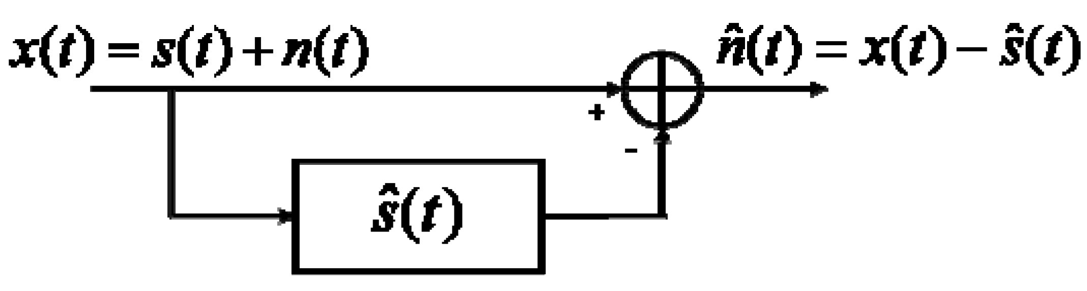
In this work we propose a different approach to mitigate the effect of RFI in microwave radiometry. It is based on the use of the power of the wavelet transform to denoise (remove noise from a signal). The interfering signal $\widehat{s}(t)$ (RFI) is estimated without any a priori knowledge of it. This signal is then subtracted from the received signal $x(t)$, to obtain a quasi RFI-free noise signal $\widehat{n}(t)=x(t)-\widehat{s}(t)$ from which the power is detected (Figure 1).

Figure 1. RFI mitigation technique: an estimate of the RFI signal $\widehat{s}(t)$ is subtracted from the received signal $x(t)=s(t)+n(t)$, so as to obtain a quasi RFI-free noise signal $\widehat{n}(t)$.

Figure 1. RFI mitigation technique: an estimate of the RFI signal $\widehat{s}(t)$ is subtracted from the received signal $x(t)=s(t)+n(t)$, so as to obtain a quasi RFI-free noise signal $\widehat{n}(t)$.

In the following sections the principles of denoising are briefly reviewed. The optimum parameters to detect and mitigate four different types of RFI (sinusoidal, Doppler-like¹, chirp², and pseudo-random noise) are studied: type of thresholding, sequence length, decomposition level, and type of wavelet (among 75 different types). In order to the study completely general and a homogeneous inter-comparison between these different signals:

• the maximum instantaneous frequency has been set to be equal to 1 Hz for all of them, so that the sequence length corresponds to the number of samples per signal period, and
• the amplitude of the different interfering signals has been properly scaled so that their power is also the same, and so the interference-to-noise (INR) ratio.

The noise power is assumed to be equal to one, and the algorithm’s performance is expressed in terms of the error of the detected output power as a function of the INR.

2. Principles of Denoising

Wavelet analysis is based in the multi-resolution analysis. Signals are decomposed into localized component waves of variable duration (wavelets). A discrete signal f is first decomposed into a first trend a1 and a first fluctuation d1: $f\to \left(a^1|d^1\right)$. Then, in the second step (or level) the first trend a1 is decomposed again into a second trend a2, and a second fluctuation d2: $f\to \left(a^2\left|d^2\right|d^1\right)$. The process is repeated a number of steps L (levels): $f\to \left(a^L\left|d^L\right|d^{L-1}\left|d^{L-2}\mathrm{...}\right|d^2|d^1\right)$. By ordering the wavelet transform coefficients by decreasing magnitude, signal compression and denoising can be performed by neglecting (or attenuating) the amplitude of the coefficients below a given threshold (see [16] for an introduction on the wavelet theory and its applications).

Consider the problem of denoising an unknown signal [17,18,19,20,21,22,23]:

$$x(t)=s(t)+n(t)$$

(1)

from a set of samples $x_i=s_i+n_i$ (i = 1,…, M) corrupted by a zero mean white Gaussian noise $n_i$. The Discrete Wavelet Transform (DWT) can be used for denoising a noisy signal. If W denotes a M by M orthonormal wavelet transformation matrix, the previous equation can be expressed in the wavelet domain as:

$$X=S+N$$

(2)

where $X\widehat{=}Wx$, $S\widehat{=}Ws$ and $N\widehat{=}Wn$ are the wavelet transforms of x, s and n. For a smooth function with additive Gaussian white noise, a theoretical threshold exists that completely removes the noise and successfully reproduces the original function:

$$\widehat{s}=W^{-1}HWx$$

(3)

where $H=diag[h(1),h(2),\mathrm{...},h(M)]$ is a filter.

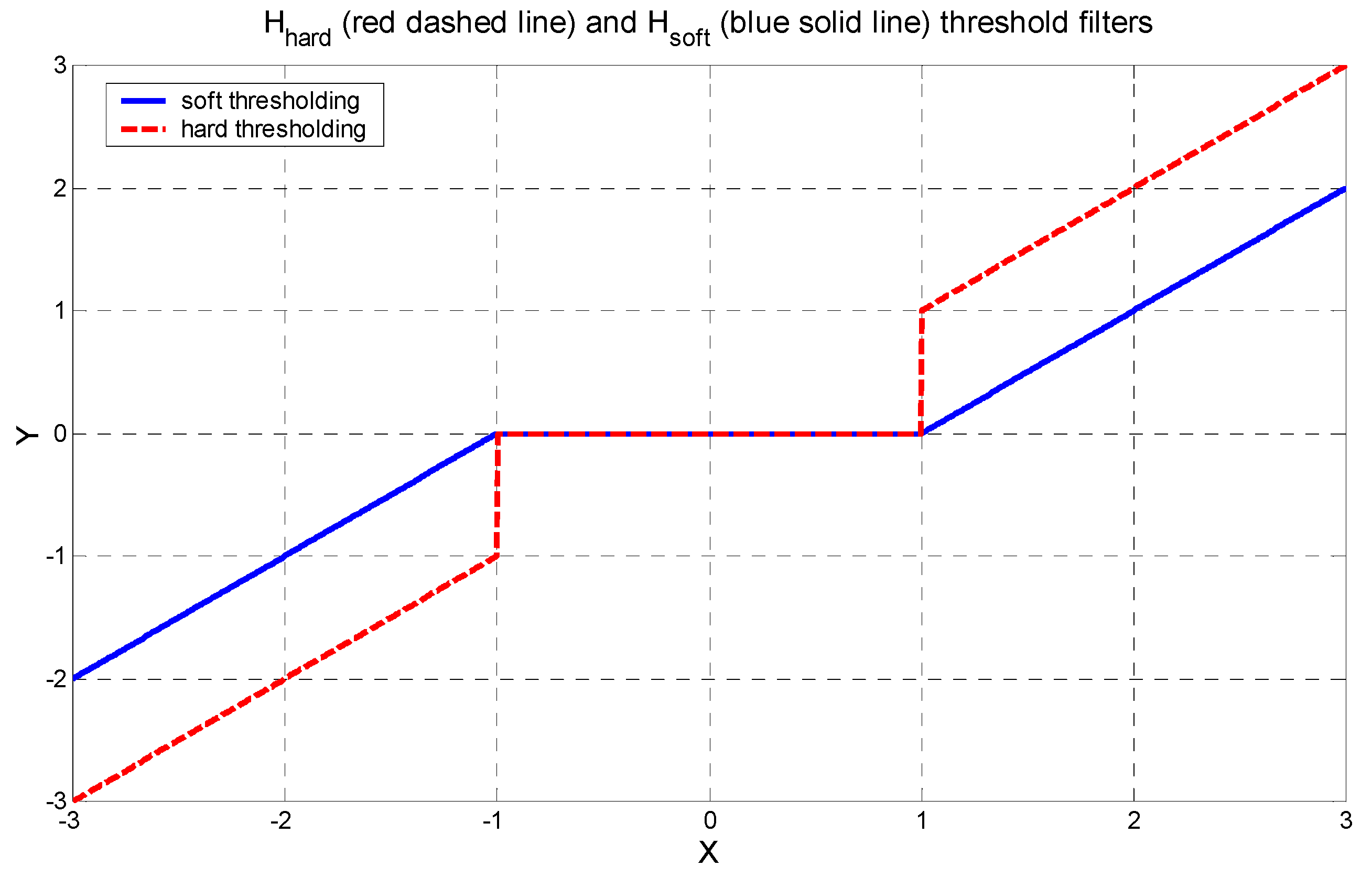
One method of filtering is thresholding. A denoised signal is obtained by applying the inverse wavelet transform $W^{-1}$ (with the same wavelet basis) to a limited number of the highest coefficients of the DWT spectrum (Y). There are a number of ways to decide which coefficients should be retained. The two simplest methods are the hard and soft thresholding:

• The hard threshold filter H_hard removes the coefficients below a threshold value T, determined by the noise variance and keeps the others to the same value:

  $$Y=X\cdot \left(\left|X\right|>T\right)$$

  (4)
• The soft threshold filter H_soft shrinks the wavelet coefficients above, and below the threshold reduces them towards zero:

  $$Y=sign(X)\cdot \left(\left|X\right|-T\right)$$

  (5)

Figure 2 shows the transfer function of the hard (red) and soft (blue) threshold filters (with T = 1). If the resulting signal has to be smooth, it has been shown that the soft threshold filter must be used [22].

Figure 2. H_hard and H_soft transfer functions of the threshold filters (with T = 1) currently used in denoising.

Figure 2. H_hard and H_soft transfer functions of the threshold filters (with T = 1) currently used in denoising.

The selection of the threshold value can be difficult. In practice, if the noise-free signal $s\left(t\right)$ is unknown, a smooth approximation of the signal is looked for. Small threshold values lead to noisy results, while large threshold values introduce bias. Experimental studies have demonstrated that for some applications, the optimal threshold is simply computed as a constant c times the noise variance [23]. Four approaches are used in this study [18]:

• One approach utilizes a selection rule based on Stein's Unbiased Risk Estimate or SURE (quadratic loss function). If the signal to noise ratio is very small, the SURE estimate is very noisy.
• The Universal method assigns a threshold level equal to the noise variance times $\sqrt{2\log \left(M\right)}$, where M is the sample size [21].
• The heuristic approach is a mixture of the two previous ones, and if the signal to noise ratio is detected to be very small, the fixed threshold is used.
• The fourth method uses a fixed threshold selected to yield the minimax performance for mean square error against an ideal procedure (minimum of the maximum mean square error).

The choice of the proper wavelet scaling function is always the most important thing. Generally, for denoising, the wavelet scaling function must have mathematical properties (shape, continuity of the signal and its derivatives) similar to the original signal. For example, to denoise pulsed signals, the Haar wavelet (box scaling function) will perform well, but it will not perform as well to denoise sinusoidal signals. On the other hand, high order Daubechies wavelets (e.g. order 8) will perform well for sinusoidal signals. If the level of decomposition increases (higher fluctuation terms d^L included), signals can be reproduced with increasingly accuracy. Therefore, a trade-off exists between the decomposition level and the complexity to evaluate the wavelet transform. The number of different wavelets is very large. See [25] for a quite detailed list of wavelet types and their properties.

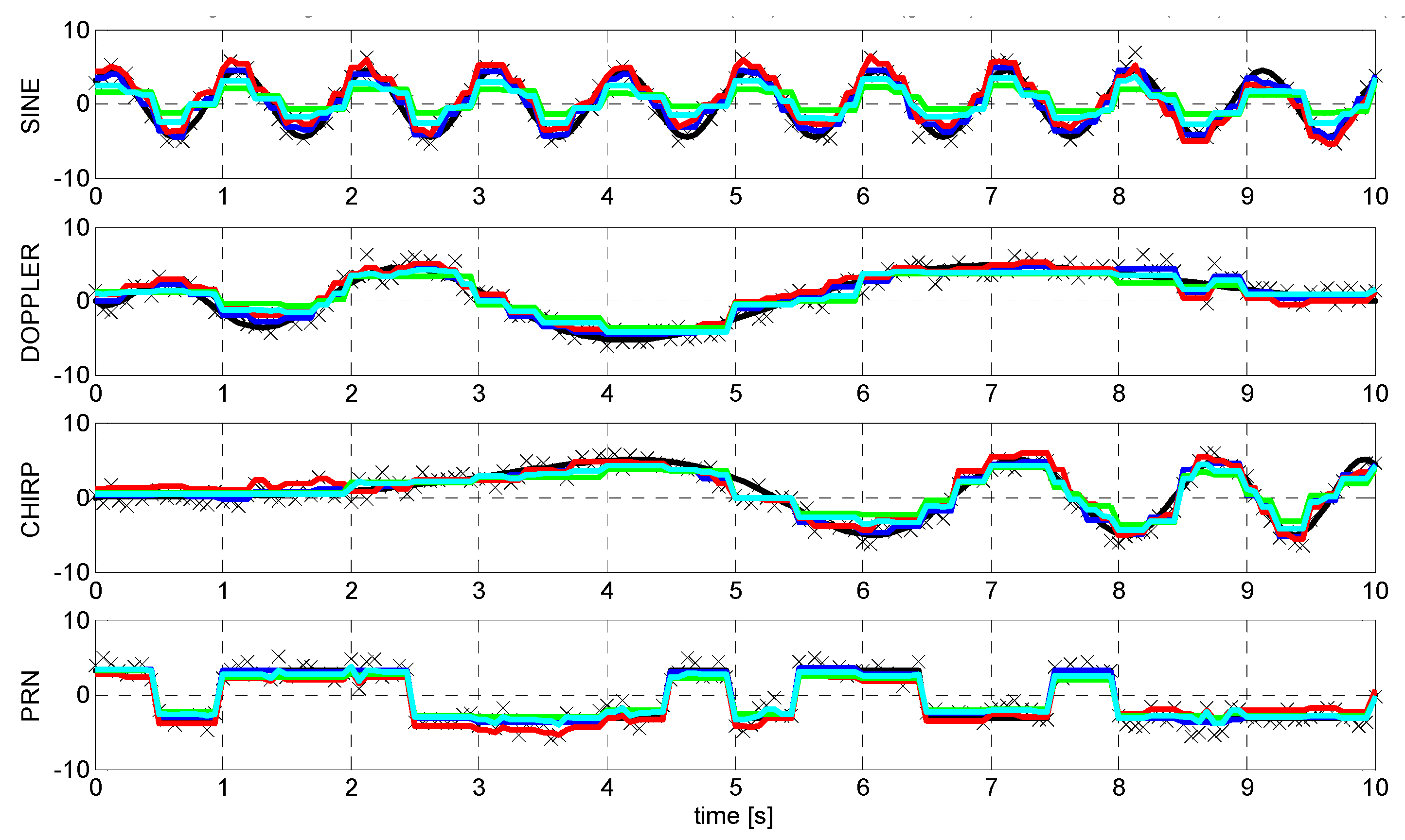
Figure 3. Original noise-free signal (black), original noisy signal (crosses), and reconstructed signals using the Haar wavelet transform, level = 12, 32 samples per period (total 320) and threshold: SURE (red), universal (green), heuristic SURE (blue) and minimax (cyan). $INR={\sigma }_{\text{interference}}^{\text{2}}/{\sigma }_{\text{noise}}^{\text{2}}=10$.

Figure 3. Original noise-free signal (black), original noisy signal (crosses), and reconstructed signals using the Haar wavelet transform, level = 12, 32 samples per period (total 320) and threshold: SURE (red), universal (green), heuristic SURE (blue) and minimax (cyan). $INR={\sigma }_{\text{interference}}^{\text{2}}/{\sigma }_{\text{noise}}^{\text{2}}=10$.

The effect of the wavelet type (Haar wavelet) and the threshold selection method can be visually seen in Figure 3 for the four different types of signals been analyzed in this work. In this case, the pseudo-random noise signal (bottom panel) is better reconstructed than the other three continuous signals.

3. Optimum Parameters Selection

In this work 75 different wavelet types have been tested [25], but simulation results (average of 100 realizations each) are presented first only for the simplest wavelet: Haar wavelet or Daubechies 1. Once the trends are understood and the optimum parameters are found for the Haar wavelet, the optimum performance for the each signal type and each wavelet type is presented.

3.1. Threshold Selection and Sequence Length

Figure 4 shows the performance of the proposed RFI mitigation wavelet technique using the Haar wavelet, as a function of the threshold methods described in Section II and the sequence length, for the four different types of interferent signals (sine, Doppler, chirp, and pseudo-random noise), decomposition level = 12, and INR = 100.

Figure 4. RFI mitigation performance using the Haar transform as a function of the threshold method and sequence length (number of samples per signal period) for four different types of interferent signals, and decomposition level = 12. Threshold method: squares = fixed threshold with single level noise estimation, circles = soft SURE, diamonds = soft heuristics SURE, and triangles = minimax. RFI signal: solid line = sine, dashed line = Doppler, dotted = chirp, and dash-dot = pseudo-random noise.

Figure 4. RFI mitigation performance using the Haar transform as a function of the threshold method and sequence length (number of samples per signal period) for four different types of interferent signals, and decomposition level = 12. Threshold method: squares = fixed threshold with single level noise estimation, circles = soft SURE, diamonds = soft heuristics SURE, and triangles = minimax. RFI signal: solid line = sine, dashed line = Doppler, dotted = chirp, and dash-dot = pseudo-random noise.

As it can be appreciated, at least 20 samples per period are required to reject RFI better than 20 dB, and as the sequence length increases, the estimated noise power error decreases (interference rejection increases) by the same factor, saturating around 3·10^-4 (INR > 55 dB) for the PRN signal at sequence lengths longer than 2¹³. In general, the fixed threshold estimation provides the worst performances, except for the SURE thresholding with the chirp signal for lengths between 64 and 1024. In general, for all signal types, the best performance is achieved using the heuristic SURE thresholding for any sequence length. Only for the PRN type of signal and below 256 samples, the minimax thresholding methods outperforms the heuristic SURE method.

3.2. Decomposition Level

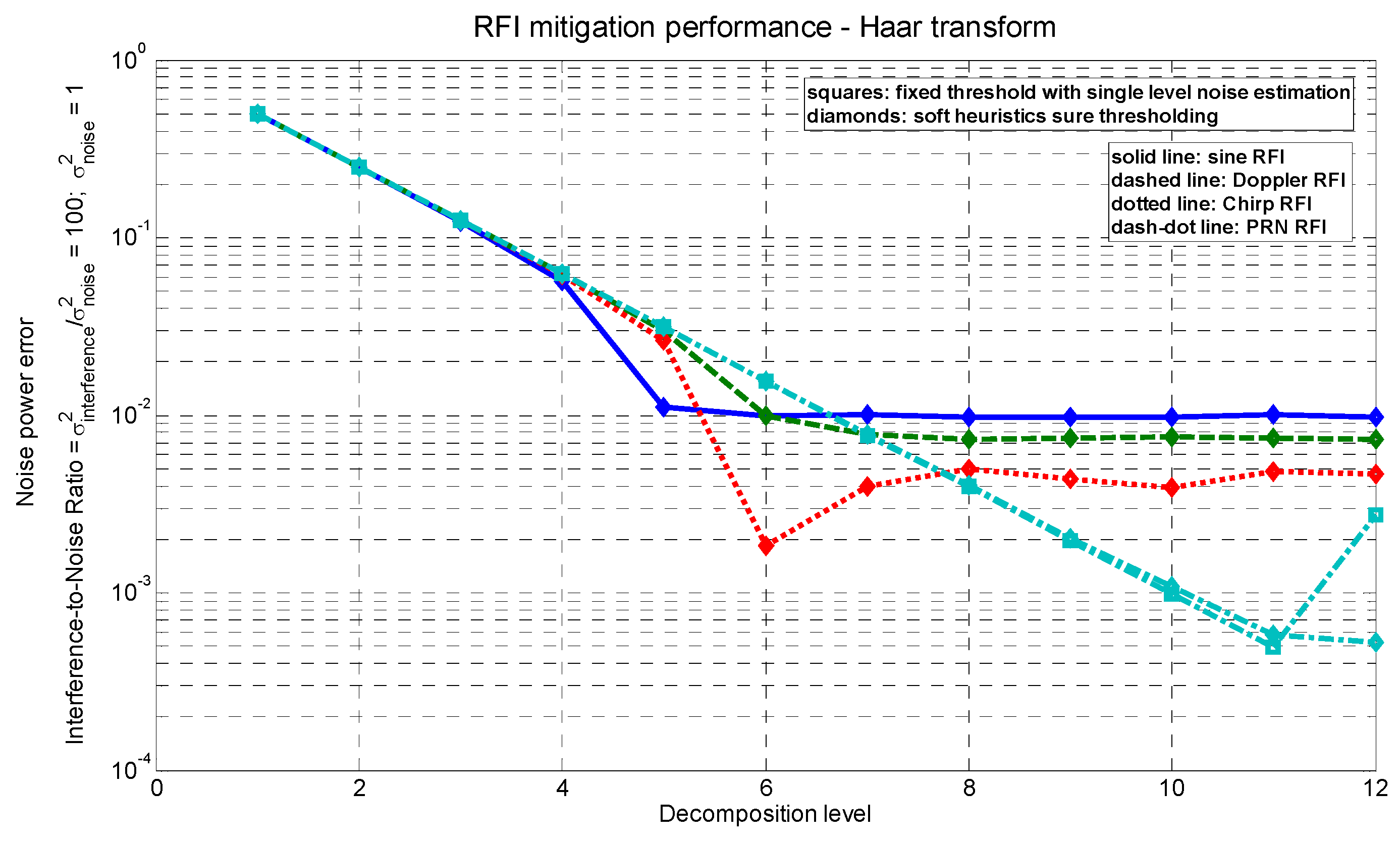
Figure 5 shows the performance of the proposed RFI mitigation wavelet technique using the Haar wavelet, with 2¹⁶ sequence length, as a function of the decomposition level. As intuitively expected, the larger the number of decomposition levels, the better the reconstruction (slope ~-1/3 decade per unit level), the smoother the function, and the smaller the number of terms in the decomposition that have to be used to reconstruct the signal properly. The quality of the reconstruction of the sinusoidal signal (and later cancellation) saturates above five levels, the Doppler signal saturates above six levels, the chirp signal saturates above seven levels, and only the PRN signals starts saturating at 11 levels. In all cases the heuristic SURE thresholding method is used, which is the one that achieves the best performance, only matched by the fixed thresholding for PRN signal.

Figure 5. RFI mitigation performance using the Haar transform as a function of the threshold method and decomposition level for four different types of interferent signals, and sequence length 2¹⁶. Threshold method: squares = fixed threshold with single level noise estimation, circles = soft SURE, diamonds = soft heuristics SURE, and triangles = minimax. RFI signal: solid line = sine, dashed line = Doppler, dotted = chirp, and dash-dot = pseudo-random noise.

Figure 5. RFI mitigation performance using the Haar transform as a function of the threshold method and decomposition level for four different types of interferent signals, and sequence length 2¹⁶. Threshold method: squares = fixed threshold with single level noise estimation, circles = soft SURE, diamonds = soft heuristics SURE, and triangles = minimax. RFI signal: solid line = sine, dashed line = Doppler, dotted = chirp, and dash-dot = pseudo-random noise.

3.3. RFI Mitigation Performance vs. Interference-to-Noise Ratio (INR)

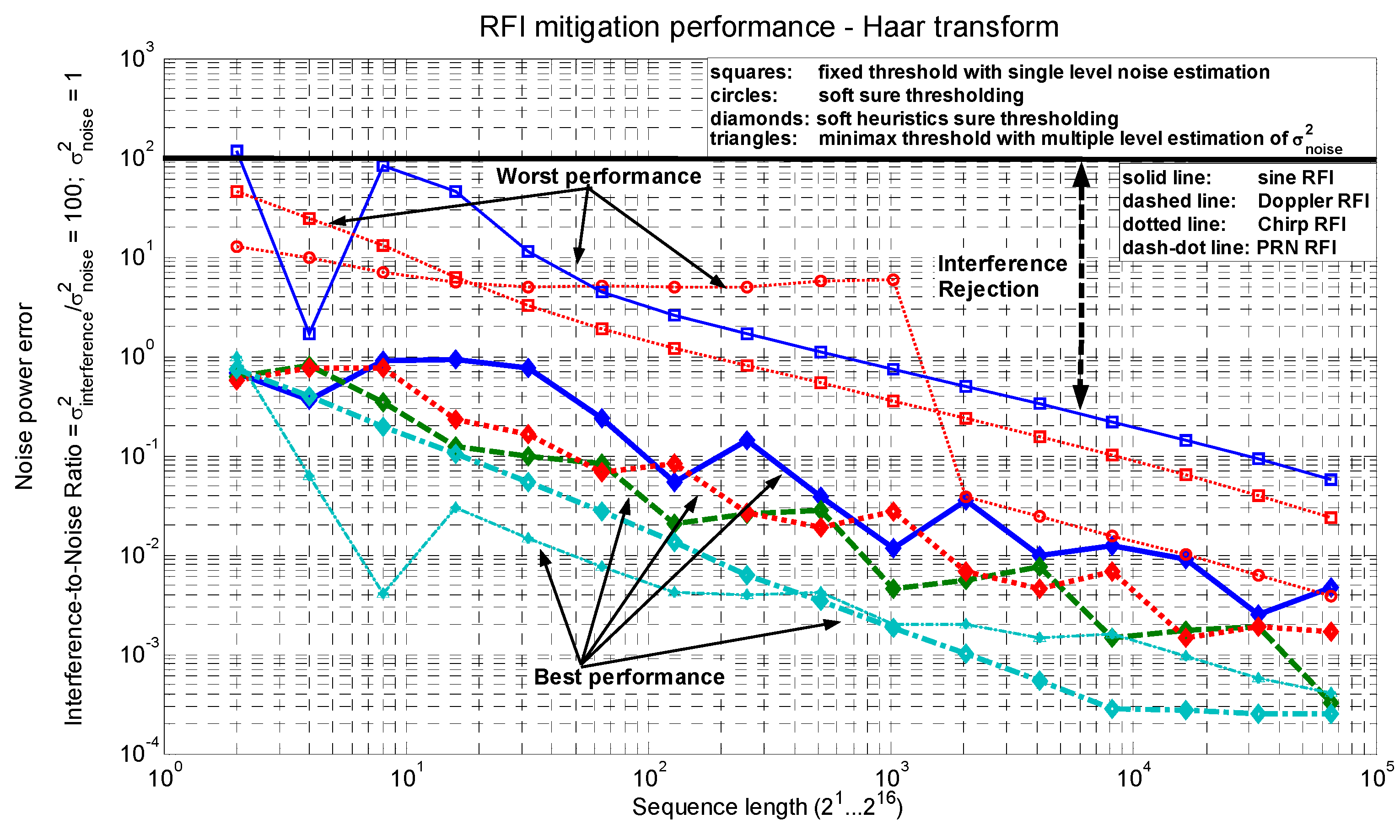
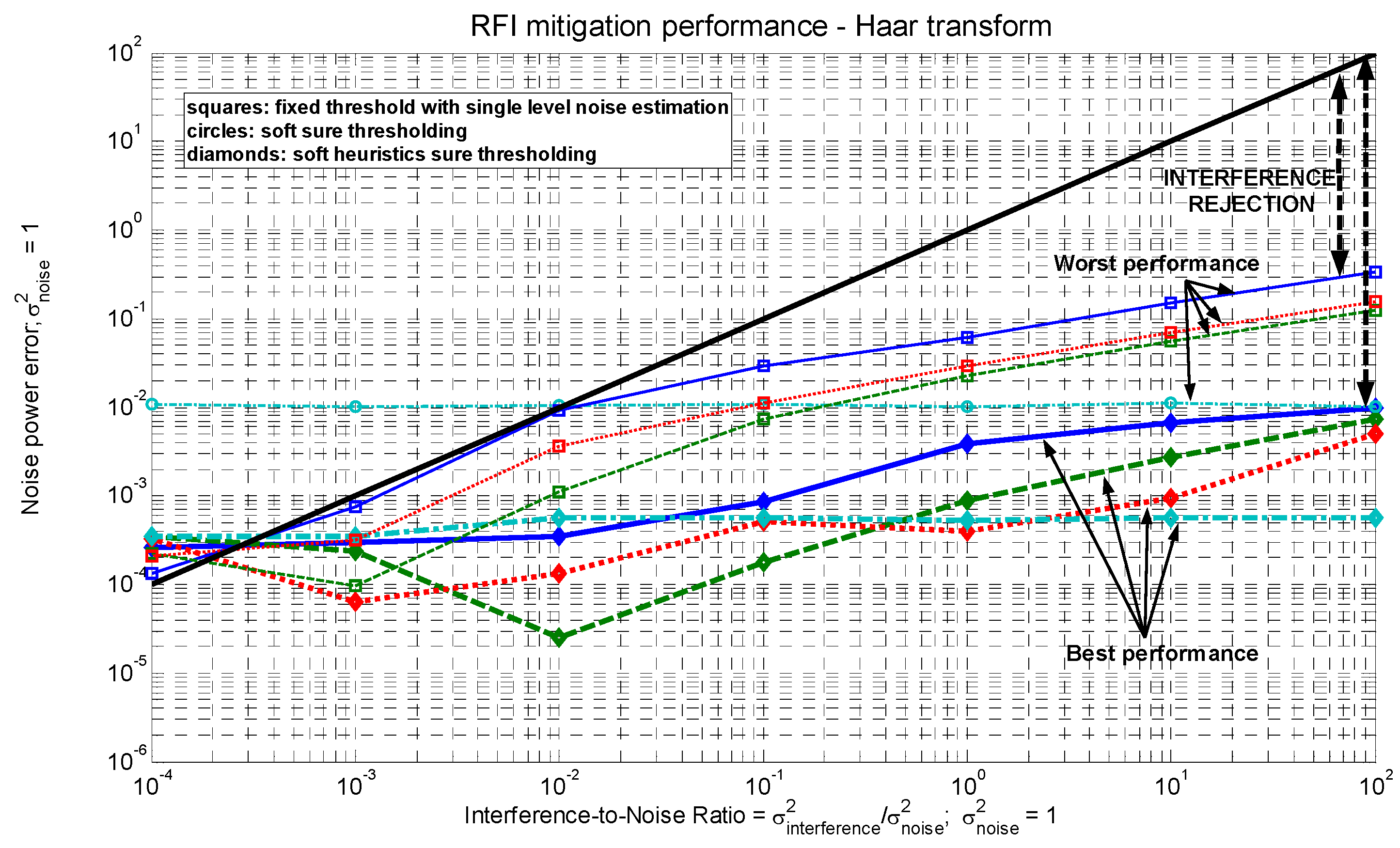
Figure 6 and Figure 7 show the RFI mitigation performance using the Haar transform or the optimum wavelet transform respectively, as a function of the threshold method and INR, for a sequence length of 2¹⁶ and a decomposition level equal to 12. As it can be appreciated, using the soft heuristic SURE thresholding the rejection is very good (~40 dB) for high INR = 100, decreasing with decreasing INR. Below INR ~ 2·10^-4 the algorithm is no longer able to estimate the RFI signal (Figure 6).

Figure 6. RFI mitigation performance using the Haar transform as a function of the threshold method and INR for four different types of interferent signals, sequence length 2¹⁶ and decomposition level = 12. Threshold method: squares = fixed threshold with single level noise estimation, circles = soft SURE, diamonds = soft heuristics SURE, and triangles = minimax. RFI signal: solid line = sine, dashed line = Doppler, dotted = chirp, and dash-dot = pseudo-random noise.

Figure 6. RFI mitigation performance using the Haar transform as a function of the threshold method and INR for four different types of interferent signals, sequence length 2¹⁶ and decomposition level = 12. Threshold method: squares = fixed threshold with single level noise estimation, circles = soft SURE, diamonds = soft heuristics SURE, and triangles = minimax. RFI signal: solid line = sine, dashed line = Doppler, dotted = chirp, and dash-dot = pseudo-random noise.

Figure 7. RFI mitigation performance using the optimum wavelet type for each signal as a function of the INR for the heuristic SURE threshold method for four different types of interferent signals, sequence length 2¹⁶ and decomposition level = 12. RFI signal: solid line = sine, dashed line = Doppler, dotted = chirp, and dash-dot = pseudo-random noise.

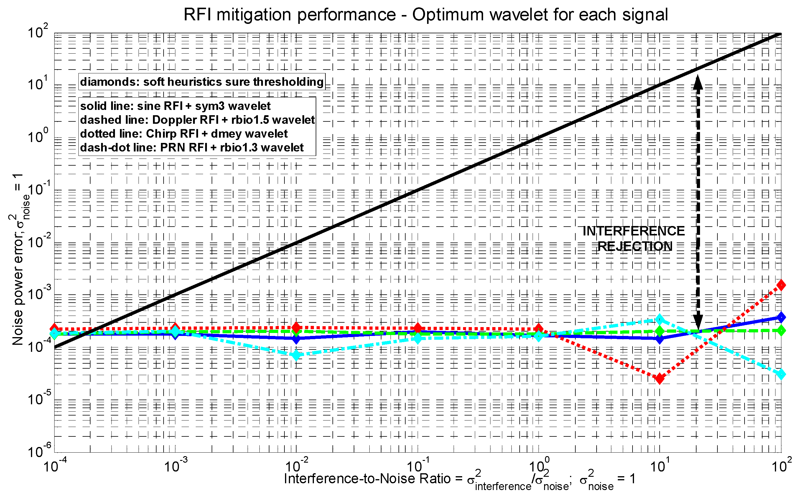
Figure 7. RFI mitigation performance using the optimum wavelet type for each signal as a function of the INR for the heuristic SURE threshold method for four different types of interferent signals, sequence length 2¹⁶ and decomposition level = 12. RFI signal: solid line = sine, dashed line = Doppler, dotted = chirp, and dash-dot = pseudo-random noise.

The optimum wavelets for each signal type have found to be the symlet 3 (sym 3) for the sinusoidal RFI, the reverse biorthogonal wavelets 1.5 (rbio1.5) for the Doppler signal, the discrete approximation of Meyer (dmey) wavelet for the chirp signal, and the reverse biorthogonal wavelets 1.3 (rbio1.3) for the PRN signals. When using the optimum wavelet types for each RFI signal the performance is significantly improved for high INRs (Figure 7), but remains stable as INR decreases so below INR ~ 2·10^-4, as in the case of the Haar wavelet, no improvement is seen.

3.4. Noise Correlation Effects

As shown in Section 3.1, at least 20 samples are required per signal period to achieve a good performance (interference rejection ≥ 20 dB) of the RFI mitigation algorithm (or 300-400 samples per period for an interference rejection ≥ 30 dB), while the Nyquist sampling rate requires just two samples per period. It is worth to address the effect of the correlation between consecutive samples introduced by the receiver’s frequency response.

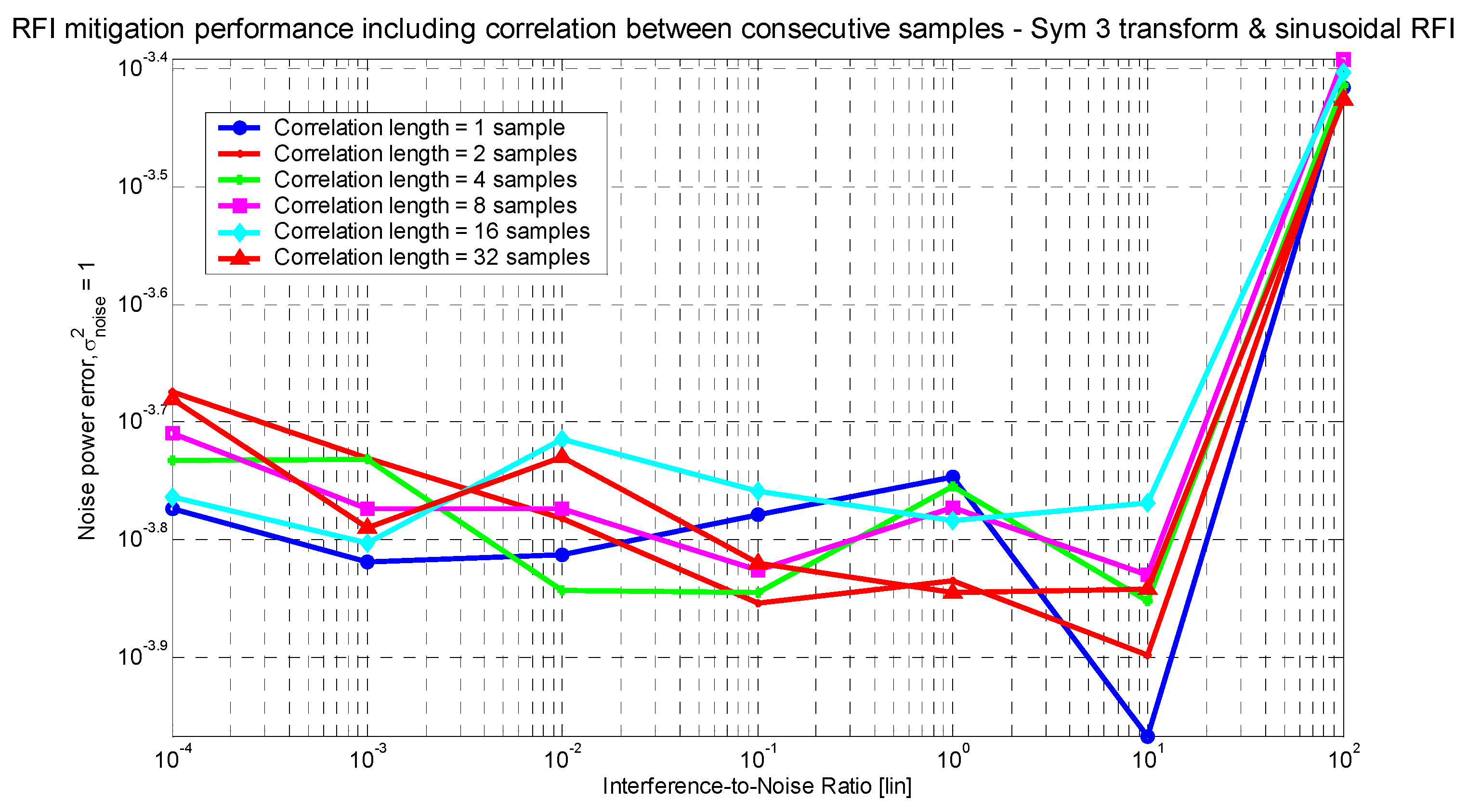
To analyze this effect, the input white noise (zero-mean random Gaussian variable) is convolved with a constant FIR (Finite Impulse Response) filter of variable length (C) and amplitude such that the variance of the output remains the same (σ²=1)³. The RFI is then added to the “colored” (filtered) noise and the wavelet-based RFI mitigation algorithm is applied. Figure 8 shows the average of 10 realizations using different correlation lengths from 1 (no correlation) up to 32. Results show that the impact of the correlation in the interference mitigation is negligible (< 0.1 dB). Results appear a bit noisy, but this is due to the small scale in the vertical axis.

Figure 8. RFI mitigation performance using the Symlet 3 wavelet transform and a sinusoidal RFI for the heuristic SURE threshold method as a function of the correlation length (in samples) of the noise. Sequence length 2¹⁶, decomposition level = 12.

Figure 8. RFI mitigation performance using the Symlet 3 wavelet transform and a sinusoidal RFI for the heuristic SURE threshold method as a function of the correlation length (in samples) of the noise. Sequence length 2¹⁶, decomposition level = 12.

3.5. Quantization Effects

So far, the analysis has been performed using floating point representation. It is worth to evaluate the impact of signal quantization in this process, since analog signals are sampled using analog-to-digital converters (ADC) with finite number of bits, and usually the higher the sampling frequency, the smaller the number of bits. To test the impact of quantization in the performance of the above-described algorithms, signals (noise + RFI) have been quantized using a variable number of bits from 4 to 16, and the ADC window has been set to ±3.5·σ. Enlarging the ADC window truncates less the input signal, better capturing the tails of the noise probability density function and –eventually- the RFI that may be present, but reduces the number of sampling levels per σ, which degrades the quality of the signal representation. Reducing the ADC window the input signal is truncated and the detected power is smaller than it actually is. With an ADC window of ±3.5·σ, the detected power is 1% less (0.99·σ²) the true input power.

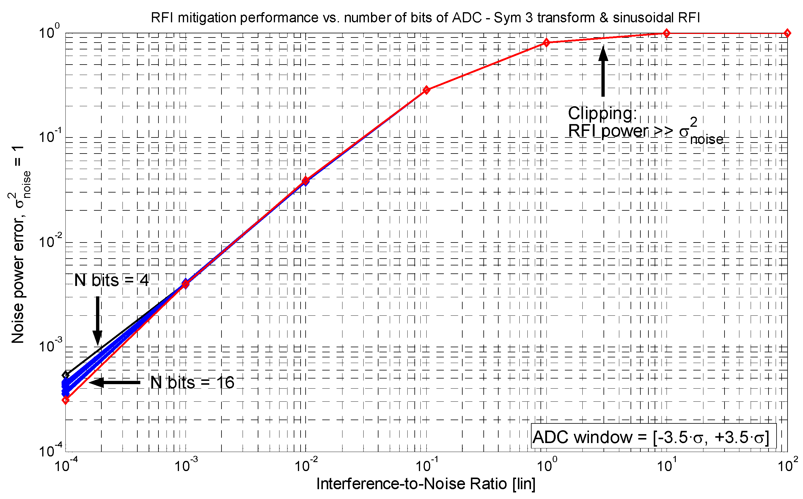
Figure 9 shows the simulation results for a sinusoidal RFI and the Symlet 3 wavelet transform. For large INR, the interference signal is so large that is clipped by the ADC and noise power error saturates to 1 (recall that noise variance is normalized to σ² = 1). Only for INR < 10^-3, the effect of the number of bits used in the quantization can be distinguished, with better performance when a larger number of bits are used in the ADC. The reason for obtaining good results with a moderate number of bits is due to the fact that noise power is estimated after integration of thousands or millions of samples (sampling frequency times the integration time). Bosch-Lluis et al. [26] demonstrated that for a ±4.05·σ ADC window and 8 bits quantization, the estimated antenna temperature error was smaller than 0.01 K, suitable for sea surface salinity measurements, while coarser quantization schemes can be used for less demanding applications.

Figure 9. RFI mitigation performance using the Symlet 3 wavelet type for a sinusoidal signal as a function of the INR for the heuristic SURE threshold method as a function of the number of bits of the analog-to-digital converter (ADC) from 4 to 16, assuming a sampling window of ±3.5·σ to minimize signal clipping in the absence of RFI. Sequence length 2¹⁶, decomposition level = 12. At high INR values of RFI clipping occurs. For larger ADC sampling windows RFI is better sampled, but noise signals suffer more from discretization effects due to the smaller number of samples per σ.

Figure 9. RFI mitigation performance using the Symlet 3 wavelet type for a sinusoidal signal as a function of the INR for the heuristic SURE threshold method as a function of the number of bits of the analog-to-digital converter (ADC) from 4 to 16, assuming a sampling window of ±3.5·σ to minimize signal clipping in the absence of RFI. Sequence length 2¹⁶, decomposition level = 12. At high INR values of RFI clipping occurs. For larger ADC sampling windows RFI is better sampled, but noise signals suffer more from discretization effects due to the smaller number of samples per σ.

4. Computing Requirements

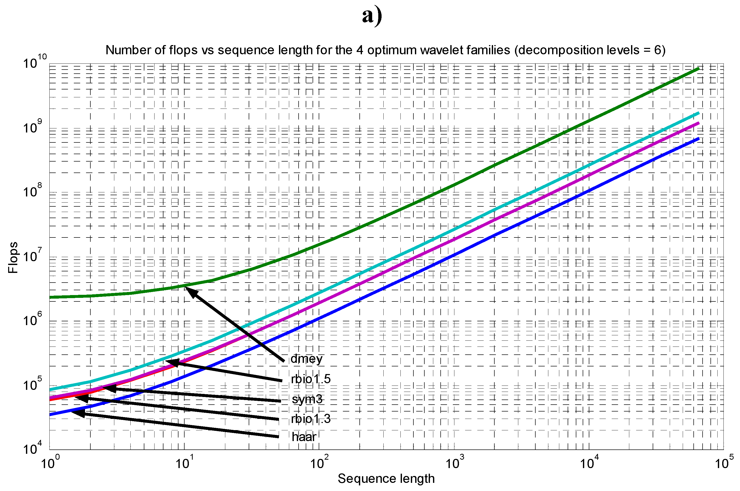
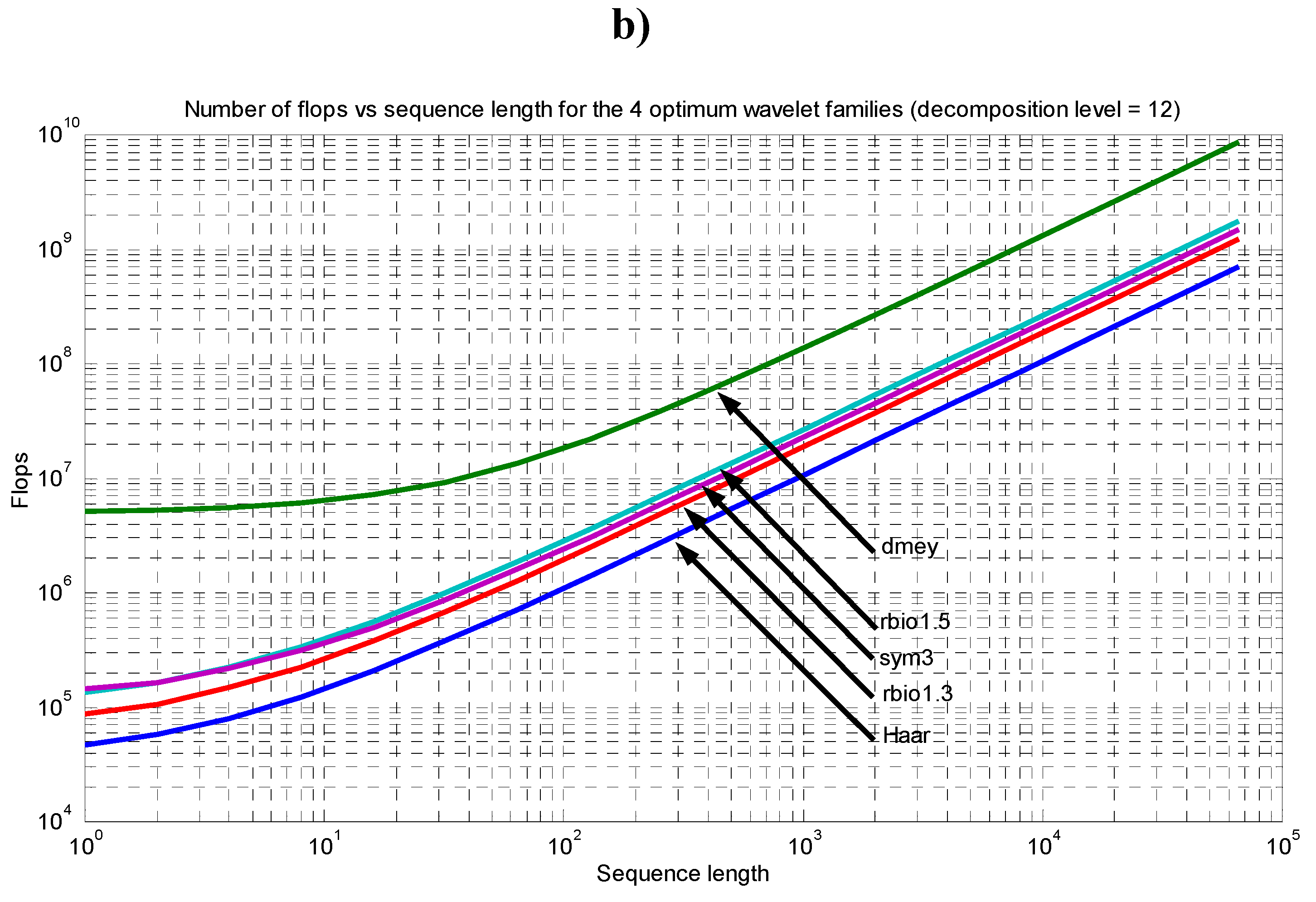
When considering the practical implementation of the described algorithms, it is critical to evaluate the number of floating operations (Flops) required. Figure 10 shows the number of floating operations required to perform the described RFI cancellation algorithm for INR = 100, as a function of the wavelet type (Haar and optimum ones in Figure 7) and the sequence length, both for decomposition levels equal to 6 (Figure 10a) and 12 (Figure 10b), for which the algorithm performance is very similar except for PRN like signals (Figure 5). Differences in the number of Flops with other INR values down to 0 (no RFI) are ≤4% and are not shown not to overload the figure.

As expected, the simplest wavelet type (Haar) is the one that requires the smallest number of Flops. On the other hand, the discrete Meyer (dmey) is the one that requires the largest number of Flops, about 10-20 times more than the Haar wavelet. For the other wavelet types (reverse biorthogonal 1.3 and 1.5 –rbio1.3 and rbio1.5-, and symlets 3 –sym3-) the number of required floating operations is about 2-3 times larger than the Haar one, which may justify its use in large RFI scenarios when the highest RFI rejection may be required (Figure 6 and Figure 7). The improved performance of the discrete Meyer transform may be questioned when balanced with the much larger computation requirements.

Below 10-20 samples length there is a saturation effect due to the computational overhead, which suggests using sequences longer than ≥20 samples. The differences between Figure 10a and Figure 10b are just a factor ≤ 2.5 for the shortest sequence lengths, being nearly identical for the sequences longer than ~10-100 samples per period.

Figure 10. Number of floating operations required by the RFI cancellation algorithm (INR = 100) vs. sequence length, for different wavelet types and decomposition levels equal to a) 6, and b) 12.

Figure 10. Number of floating operations required by the RFI cancellation algorithm (INR = 100) vs. sequence length, for different wavelet types and decomposition levels equal to a) 6, and b) 12.

Assuming a system operating at L-band (1.400-1.427 MHz) that acquires 20 samples per period to warrant enough RFI rejection (Figure 4), the sampling rate is 20 samples/period · 27·10⁶ periods /s = 540 Msamples/s. Unfortunately, this high data rate cannot be processed with today’s spaceborne processors (e.g. 4 MFlops/s with Leon 3 [27]) or even ground-based FPGAs [28]. However, the proposed algorithm can be applied either at intermediate frequency or for the in-phase and quadrature components of the demodulated signal separately, to reduce the signal bandwidth by a factor of 2 and accordingly the computing requirements per processor, at the expense of doubling the number of processors. Further reductions can be achieved by sub-banding (dividing the original band into smaller ones) and applying the proposed algorithm to each of the sub-bands.

5. Conclusions

A RFI mitigation algorithm has been presented. It is based on the estimation of the RFI signal using wavelet denoising techniques, and its subtraction from the original signal so as to obtain an estimate of the noise-only signal.

It has been found that in general, the soft heuristic SURE thresholding method is the one that best performs for any type of signal, except for very weak RFI (INR ~ 10^-3 … 10^-4) in which the fixed thresholding performs slightly better.

The minimum number of samples per period is ~20, for which at least a ≥20 dB interference rejection is achieved using the Haar transform (depending on the signal type and the thresholding method). Higher rejections (≥40 dB) are achieved at the expense of longer sequences (2¹⁶ samples) and increased computational load (~3·10⁵ Flops for 20 samples/period to 7·10⁸ Flops for 2¹⁶ samples/period, Figure 10a). Increasing the number of decomposition levels above 6-7 does not improve the quality of the RFI mitigation, except for PRN (pulsed) signals.

The minimum inteference rejection (cancellation) is ~40 dB for high INRs (INR~100) when using the Haar wavelet transform, but this value may increase up to ~60-70 dB if the optimum wavelet type for each signal is selected: symlet 3 for the sinusoidal RFI, the reverse biorthogonal wavelets 1.5 for the Doppler signal, the discrete approximation of Meyer wavelet for the chirp signal, and the reverse biorthogonal wavelets 1.3 for the PRN signals. Therefore there is a trade-off between interference rejection and computational complexity which must be evaluated depending on the application.

Even in the case of using the simple Haar transform, the proposed RFI mitigation algorithm allows one to make useful radiometric measurements in areas heavily corrupted by RFI. Since it is unlikely that with today’s computers and FPGAs this technique can be applied for real time processing in microwave radiometers, the RFI cancellation could be applied a posteriori to the recorded data. This can be of special interest in scenarios corrupted by human activity where the errors induced by RFI are equal or larger than the measurement uncertainty (ΔT) and blanking is not an option due to the data loss. For example, if the antenna temperature is 100 K, the receivers noise temperature is 300 K, and the measurement uncertainty is ΔT = 1 K, the minimum detectable power is 1 K/(100 K + 300 K) = 2.5·10^-3 (assuming σ² = 1), which determines the minimum useful INR for which it makes sense to apply the RFI mitigation algorithm. In other demanding applications, such as sea surface salinity retrieval, where the required ΔT is much smaller (ΔT = 0.05 K), RFI mitigation can be useful down to INR of ~0.05 K/(100 K +300 K) ≅ 10^-4, which is at the limit of the performance of the RFI cancellation algorithm, regardless of the wavelet type used.

References and Notes

- Njoku, E.G.; Ashcroft, P.; Chan, T.K.; Li, L. Global survey and statistics of radio-frequency interference in AMSR-E land observations. IEEE T. Geosci. Remote 2005, 43, 938–947. [Google Scholar] [CrossRef]
- Ellingson, S.W.; Johnson, J.T. A Polarimetric Survey of Radio-Frequency Interference in C- and X-Bands in the Continental United States Using WindSat Radiometry. IEEE T. Geosci. Remote 2006, 44, 540–548. [Google Scholar] [CrossRef]
- Younis, M.; Maurer, J.; Fortuny-Guasch, J.; Schneider, R.; Wiesbeck, W.; Gasiewski, A.J. Interference from 24-GHz Automotive Radars to Passive Microwave Earth Remote Sensing Satellites. IEEE T. Geosci. Remote 2007, 42, 1387–1398. [Google Scholar] [CrossRef]
- Ellingson, S.W.; Hampson, G.A.; Johnson, J.T. Design of an L-Band Microwave Radiometer with Active Mitigation of Interference. In Proceedings of IEEE International Geoscience and Remote Sensing Symposium IGARSS 2003; Volume 3, pp. 1751–1753.
- Guner, B.; Johnson, J.T.; Niamswaun, N. Time and frequency blanking for radio frequency interference mitigation in microwave radiometry. IEEE T. Geosci. Remote 2007, 45, 3672–3679. [Google Scholar] [CrossRef]
- Johnson, J.T.; Gasiewski, A.J.; Guner, B.; Hampson, G.A.; Ellingson, S.W.; Krishnamachari, R.; Niamsuwan, N.; McIntyre, E.; Klein, M.; Leuski, V.Y. Airborne radio-frequency interference studies at C-band using a digital receiver. IEEE T. Geosci. Remote 2006, 44, 1974–1985. [Google Scholar] [CrossRef]
- Ruf, C.S.; Gross, S.M.; Misra, S. RFI detection and mitigation for microwave radiometry with an agile digital detector. IEEE T. Geosci. Remote 2006, 44, 694–706. [Google Scholar] [CrossRef]
- De Roo, R.D.; Misra, S.; Ruf, C.S. Sensitivity of the Kurtosis Statistic as a Detector of Pulsed Sinusoidal RFI. IEEE T. Geosci. Remote 2007, 45, 1938–1946. [Google Scholar]
- Misra, S.; Ruf, C.S. Detection of Radio-Frequency Interference for the Aquarius Radiometer, IEEE T. Geosci. Remote 2008, 46, 3123–3128. [Google Scholar] [CrossRef]
- De Roo, R.D.; Misra, S. Effectiveness of the Sixth Moment to Eliminate a Kurtosis Blind Spot in the Detection of Interference in a Radiometer. IEEE International Geoscience and Remote Sensing Symposium 2008, IGARSS 2008. Volume 2, 331–334. [Google Scholar]
- Johnson, J.T.; Potter, L.C. Performance Study of Algorithms for Detecting Pulsed Sinusoidal Interference in Microwave Radiometry. IEEE T. Geosci. Remote 2009, 47, 628–636. [Google Scholar] [CrossRef]
- Piepmeier, J.R.; Mohammed, P.N.; Knuble, J.J. A Double Detector for RFI Mitigation in Microwave Radiometers. IEEE T. Geosci. Remote 2008, 46, 458–465. [Google Scholar] [CrossRef]
- Fridman, P.A.; Baan, W.A. RFI methods in radiastronomy. Astronomy and Astrophysics 2001, 378, 327–344. [Google Scholar] [CrossRef]
- Middleton, D. Non-Gaussian noise models in signal processing for telecommunications: New methods and results for Class A and Class B noise models. IEEE T. Inform. Theory 1999, 45, 1129–1149. [Google Scholar] [CrossRef]
- Evans, B.L. Mitigation of Radio Frequency Interference from the Computer Platform to ImproveWireless Data Communication. Intel Labs Seminar – University of Texas. 16 April 2007. http://users.ece.utexas.edu/~bevans/projects/rfi/talks/April2007.html.
- Walker, J.S. A Primer on Wavelets and Their Scientific Applications, 2nd ed.; Chapman & Hall/CRC: Boca Raton, FL, USA, 2008; Chapters 1-2. [Google Scholar]
- Donoho, D.L. De-Noising by soft-thresholding. IEEE T. Inform. Theory 1995, 41, 613–627. [Google Scholar] [CrossRef]
- MATLAB tutorial on denoising: http://www.mathworks.com/access/helpdesk/help/toolbox/ wavelet/index.html?/access/helpdesk/help/toolbox/wavelet/ch06_a12.html&http://www.mathworks.com/access/helpdesk/help/toolbox/wavelet/ch06_a10.html#62573.
- Misiti, M.; Misiti, Y.; Oppenheim, G.; Poggi, J.M. Wavelet Toolbox User's Guide; The MathWorks Inc.: Natick, MA, USA, 1996. [Google Scholar]
- Aboufadel, E.; Schlicker, S. Discovering Wavelets; John Wiley and Sons: New York, NY, USA, 1999; p. 14. [Google Scholar]
- Donoho, D.L.; Johnstone, I.M. Ideal spatial adaption by wavelet shrinkage. Biometrika 1994, 81, 425–455. [Google Scholar] [CrossRef]
- Ghael, S.P.; Sayeed, A.M.; Baraniuk, R.G. Improved Wavelet Denoising via Empirical Wiener Filtering. In Proceedings of SPIE, Mathematical Imaging, San Diego, CA, USA, July 1997; Vol. 3169, pp. 389–399.
- Lang, M.; Guo, H.; Odegard, E.; Burrus, C.S.; Wells, R.O. Nonlinear processing of a shift-invariant discrete wavelet transform (DWT) for noise reduction. Harold, H. Szu, Ed.; 1995; Vol. 2491, pp. 640–651. [Google Scholar]
- Resnikoff, H.; Wells, R.O. Wavelet Analysis: The Scalable Structure of Information; Springer-Verlag: New York, NY, USA, 2002; p. 365. [Google Scholar]
- Summary of wavelet families and properties: http://www.mathworks.com/access/helpdesk/help/ toolbox/wavelet/index.html?/access/helpdesk/help/toolbox/wavelet/ch06_a12.html&http://www.mathworks.com/access/helpdesk/help/toolbox/wavelet/ch06_a10.html#62573/.
- Leon 3 description: http://www.gaisler.com/cms/index.php?option=com_content&task=view& id=196&Itemid=172.
- Bosch-Lluis, X.; Ramos-Pérez, I.; Camps, A.; Marchan-Hernandez, J.F.; Rodríguez-Álvarez, N.; Valencia, E.; Vericat, M.; Guerrero, M. A. The Impact of the Number of Bits in Digital Beamforming Real Aperture and Synthetic Aperture Radiometers. In Proceedings of the Microwave Radiometry and Remote Sensing of the Environment, MICRORAD 2008, Florence, Italy, 11–14 March 2008.
- Elfouly, F.E.; Mahmoud, M.I.; Dessouky, M.I.M.; Deyab, S. Comparison between Haar and Daubechies Wavelet Transformations on FPGA Technology. IJCISSE 2008, 2, 37–42. [Google Scholar]
© 2009 by the authors; licensee Molecular Diversity Preservation International, Basel, Switzerland. This article is an open-access article distributed under the terms and conditions of the Creative Commons Attribution license (http://creativecommons.org/licenses/by/3.0/).
Share and Cite
MDPI and ACS Style
Camps, A.; Tarongí, J.M. RFI Mitigation in Microwave Radiometry Using Wavelets. Algorithms 2009, 2, 1248-1262. https://doi.org/10.3390/a2031248
AMA Style
Camps A, Tarongí JM. RFI Mitigation in Microwave Radiometry Using Wavelets. Algorithms. 2009; 2(3):1248-1262. https://doi.org/10.3390/a2031248
Chicago/Turabian StyleCamps, Adriano, and José Miguel Tarongí. 2009. "RFI Mitigation in Microwave Radiometry Using Wavelets" Algorithms 2, no. 3: 1248-1262. https://doi.org/10.3390/a2031248