3.1. Executions of Extended-Lazy for insertions
As summarized in
Figure 4, the behavior of
Extended-Lazy for an insertion
is divided into six cases based on the status of the level
.
Figure 4.
Execution of Extended-Lazy for an insertion .
Figure 4.
Execution of Extended-Lazy for an insertion .
Case (1): The case that does not belong to a tank and is rich. Execute AppendRich(). The execution of this case costs 1 and the number of locally rich levels increases by at most one because only changes its status.
Case (2): The case that does not belong to a tank and is poor. Furthermore, if we look at the higher levels than in the order of until we encounter a level that is rich or a bottom of a tank, we encounter a rich level (say, the level t) before a bottom of a tank. In this case, execute AppendRich(). Note that the new tank[] is created. This case costs 1 and the number of locally rich levels increases by at most one since only level t changes its status.
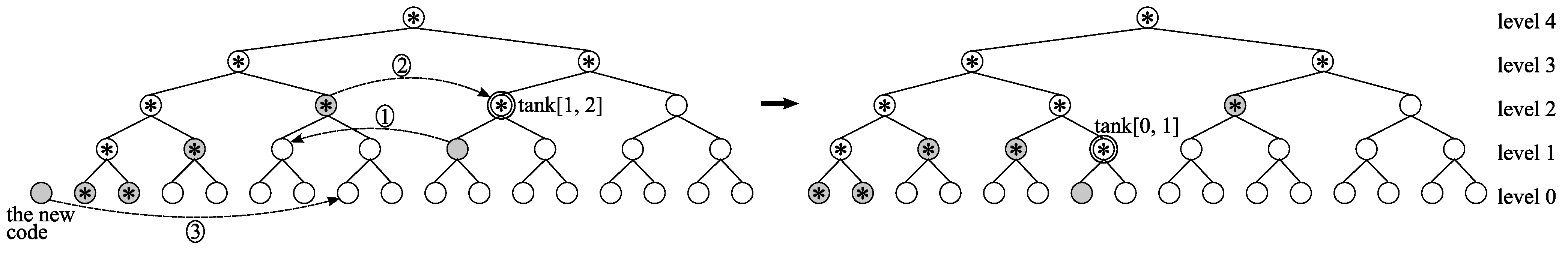
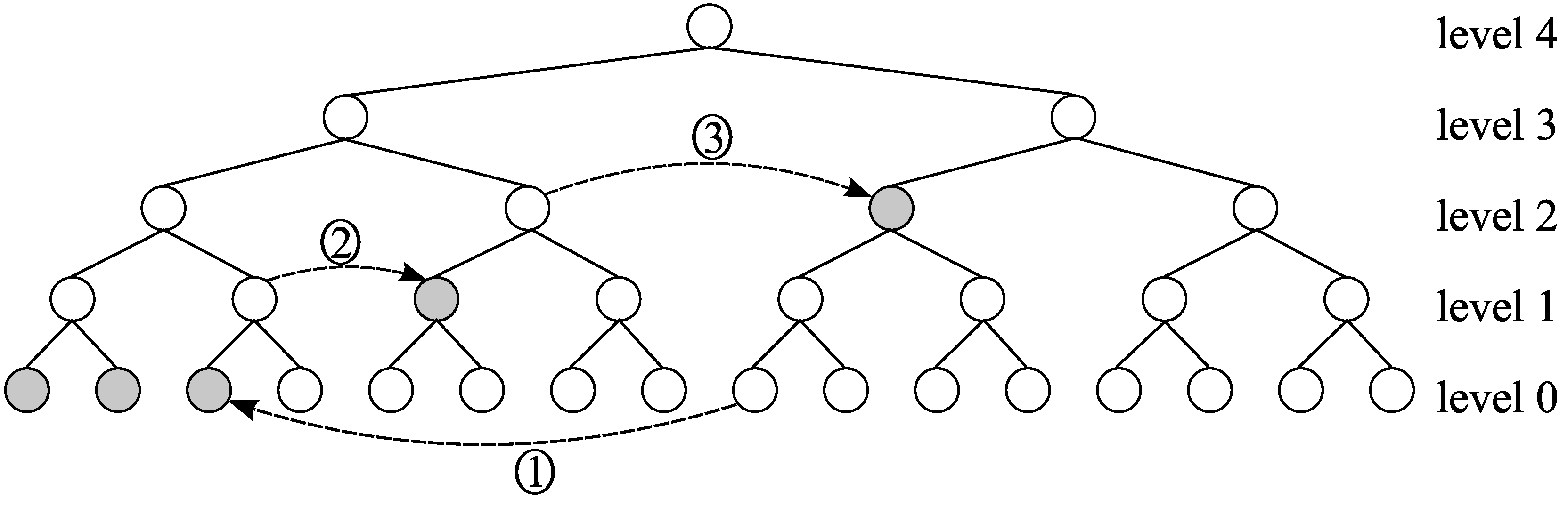
Case (3): The same as Case (2), but when looking at higher levels, we encounter a bottom
b of tank[
] before we encounter a rich level. Since this case is a little bit complicated, we give an example in
Figure 5, in which
,
, and
. First, execute FreeTail(
t) and receive the code
of level
b (because a level-
b code was assigned to level
t by exploiting a tank), and then execute AppendPoor(
) (note that
b is poor by the condition (v) of semi-compactness)(
Figure 5①). Next, receive another code
of level
s. Note that there is an assigned vertex at
t because of the condition (iv), and hence
. Then, using AppendRich(
), assign
to the vertex which was tank[
], which creates the new tank[
] if
(
Figure 5②). Now, recall that the level
b was poor, and hence
was assigned to a left child. So, the level
b is currently locally rich. We execute AppendRich(
) (
Figure 5③). Note that tank[
] is newly created. In this case, the cost incurred is 3, and the number of locally rich levels does not change.
Figure 5.
An execution of Case (3).
Figure 5.
An execution of Case (3).
Case (4): The case that is the top of a tank and is rich. First, execute FreeTail() and receive the code from the bottom of the tank. Then, execute AppendRich() and AppendRich() in this order. Intuitively speaking, we shift the top of the tank to the right, and assign c to the vertex which was the tank. In this case, it costs 2 and similarly as Case (1), the number of locally rich levels increases by at most one.
Case (5): The case that is the top of a tank, say tank[], and is poor. Execute FreeTail() and receive the code of level b from tank[], and execute AppendRich() to process c. Note that is poor because was the bottom of tank[]. Also, note that b currently does not belong to a tank. Hence our current task is to process of level b where b does not belong to a tank and is poor. So, according to the statuses of levels higher than b, we execute one of Cases (2) or (3). Before going to Cases (2) or (3), the cost incurred is 1 and there is no change in the number of locally rich levels. Hence, the total cost of the whole execution of this case can be obtained by adding one to the cost incurred by the subsequently executed case (Cases (2) or (3)), and the change in the locally rich levels is the same as that of the subsequently executed case.
Case (6): The case that belongs to tank[] and is not the top of tank[]. Execute FreeTail(t) and receive the code of level b from tank[]. Then, execute AppendPoor() and receive a code of level s. By a similar observation as Case (3), we can see that . Then, assign to the vertex which was tank[] using AppendRich(). (Note that tank[] is created if .) Since was poor, c was assigned to a left child. Hence is currently locally rich. Execute AppendRich(), which creates tank[b, ] if . The execution of this case costs 3, and the number of locally rich levels does not change.
Here we give one remark. Suppose that does not belong to a tank and is poor. Then, we look at higher levels to see which of Cases (2) and (3) is executed. But, it may happen that we encounter neither a rich level nor a bottom of a tank, namely there is no tank in upper levels and all the upper levels are poor. We define this case as Case (7). However, we can prove the following lemma.
Lemma 1. If the semi-compactness is preserved and Case (7) occurs, then there is no configuration that assigns all the current codes.
Proof. We define the bandwidth of a cade c as and the bandwidth of the OVSF code tree of hight h as . Suppose that the semi-compactness is preserved and Case (7) occurs when an insertion arrives. We show that , the bandwidth required by this request, exceeds the bandwidth of the tree not used by the currently assigned codes.
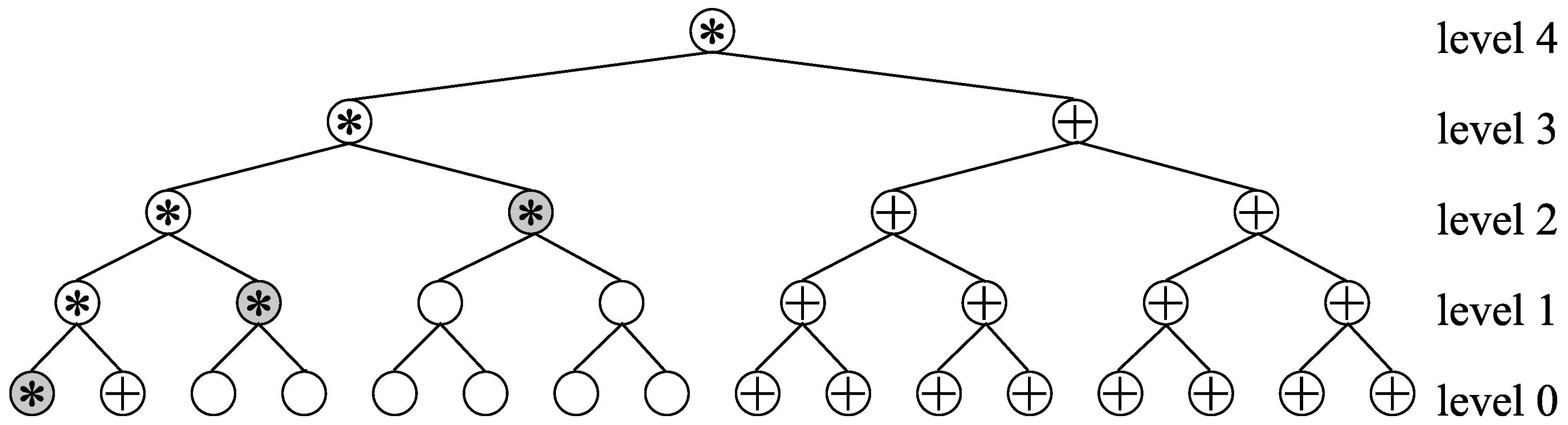
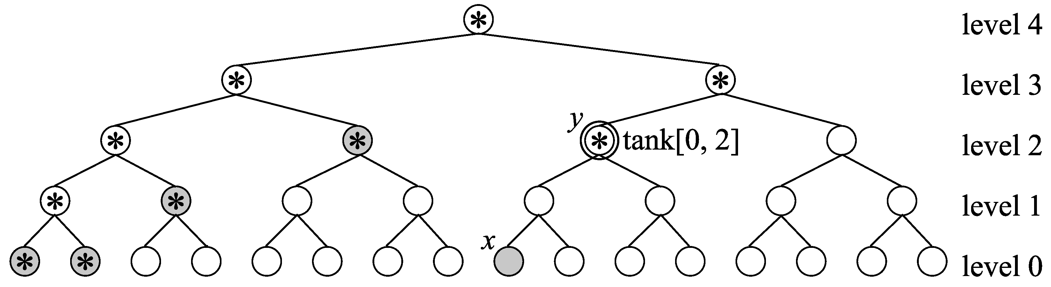
First, we transform the semi-compact assignment to a compact assignment. We remove tanks from the semi-compact assignment. Consider tank[]. Release the code of level b from tank[] temporarily. Then, assign to the vertex v immediately right of the rightmost dead vertex at b. Because of conditions (ii) and (v) of semi-compactness, b is poor and the path from v to the root includes exactly one assigned vertex at some level . Release code assigned to and assign to the vertex immediately right of the rightmost dead vertex at ℓ. By repeating the above operations, a code assigned to a vertex at level t is released. ( exists because of condition (iv) of semi-compactness.) We assign to the vertex which was tank[].
We show that conditions of semi-compactness remain satisfied after the above operation. Conditions (iii), (iv), and (v) remain satisfied for the levels which did not belong to tank[] because no code was released from nor assigned to these levels. Also, conditions (iii), (iv), and (v) remain satisfied for levels which belonged to tank[] because these conditions state on levels that belong to tanks but these levels do not belong to a tank any more since tank[] was removed. (This argument is used several times in the later proofs.)
Condition (i) remains satisfied because once two codes overlap, the one, say c, at the higher level is moved immediately. Suppose that c is moved from to in this step. Then, becomes unassigned but is still dead because one of its descendants is assigned. Also, was the leftmost non-dead vertex at level . Hence, Condition (ii) remains satisfied.
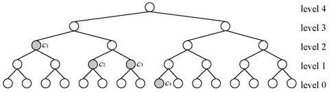
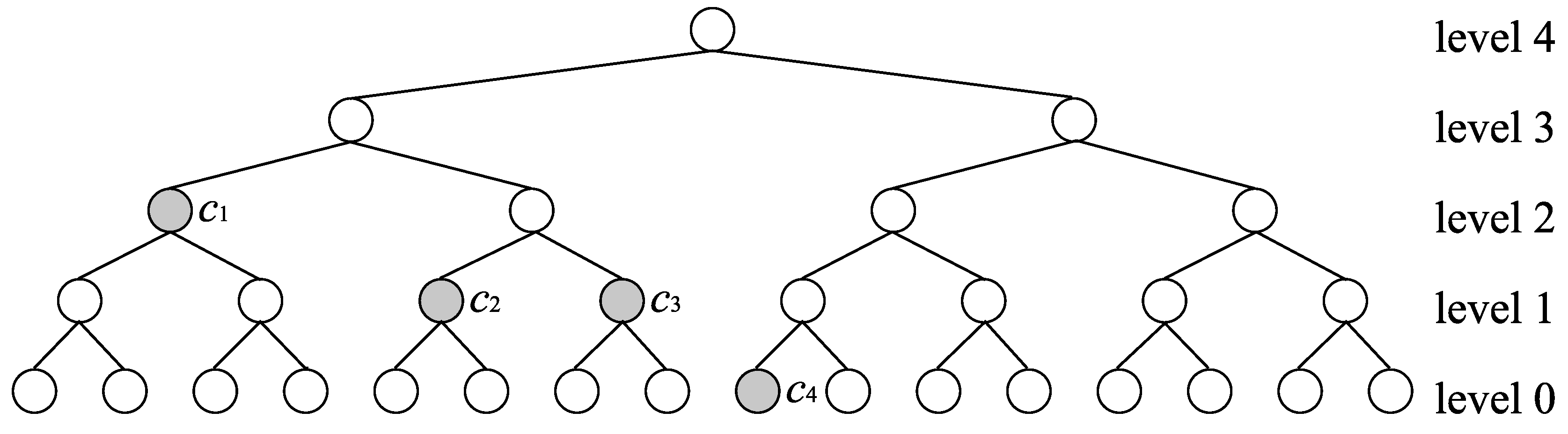
If we do the above operation for each tank independently, the initial semi-compact assignment is transformed to a semi-compact assignment with no tanks. By definition, a semi-compact assignment with no tanks is a compact assignment. For example, the semi-compact assignment in
Figure 3 is transformed to the compact assignment in
Figure 6.
Figure 6.
Transformation from a semi-compact assignment to a compact assignment.
Figure 6.
Transformation from a semi-compact assignment to a compact assignment.
Since the levels and higher remain poor, there is no vertex of level which c can be assigned to and the bandwidth which is not used at the levels and higher is 0. Then, we calculate the bandwidth which is not used at the levels lower than . We call the vertex v a free-root if v and its all the children are assignable, and its parent is not assignable. Let T denote the set of free-roots. The non-used bandwidth is the total bandwidth of the vertices of T. Each free-root should be the right child of its parent. For, if a free-root is the left child of its parent p, the right child of p is also assignable because of the compactness. Therefore, p is assignable, which contradicts the definition of free-root. Suppose that there are more than one free-roots f and at the same level ℓ, and suppose that lies to the right of f. As discussed above, both f and are the right children of their parents. Since both f and are assignable (and non-dead), all vertices between them are non-dead because of the compactness. In particular, the vertex immediately left of is non-dead. Since is assignable and is non-dead, the parent of and has no assigned descendants. Moreover, since is assignable, has no assigned ancestors. Then is assignable, which again contradicts the definition. Hence, in a compact assignment, there is at most one free-root at each level. The total bandwidth is then at most , which is smaller than . ☐
As we have mentioned previously, we excluded inputs in which the total bandwidth of all codes which should be assigned exceeds the capacity. Hence, Case (7) does not occur if the semi-compactness is preserved. (Actually, we do not have to exclude this case because our algorithm preserves the semi-compactness and detects this situation, and in such a case, our algorithm can simply reject the insertion.)
The following lemma proves the correctness of Extended-Lazy on insertions.
Lemma 2. Extended-Lazy preserves the semi-compactness on insertions.
Proof. In order to prove this lemma, we have to show that the five conditions (i) through (v) of semi-compactness are preserved after an insertion is served. It is relatively easy to show that (i) is preserved because Extended-Lazy uses only AppendRich, AppendPoor, and FreeTail, each of which preserves the orthogonality even by a single application. So, we show that conditions (ii) through (v) are satisfied after the execution of each of Cases (1) through (6), provided that (i) through (v) are satisfied before the execution.
Case (1): It is not hard to see that conditions (iii) through (v) remain satisfied because no tank is created or removed. We check that condition (ii) is satisfied for each group of levels , , and .
| : | Condition (ii) remains satisfied because nothing changes. |
| : | Since we only append c to the leftmost non-dead vertex at , condition (ii) remains satisfied. |
| : | Let v be the vertex to which the code c is assigned. Note that by AppendRich(), some of ancestors of v may turn from non-dead to dead. Suppose that vertex of level s () turned from non-dead to dead. Then, by the above observation, is an ancestor of v. Next, let be the vertex which is immediately left of v. Then, since was dead, is not an ancestor of . As a result, the ancestor of at level s is the vertex, say , immediately left of , which implies that was dead. Thus, condition (ii) remains satisfied at any level. |
Case (2): We can see that condition (ii) is satisfied by a similar discussion as Case (1). The tank tank[] is only the tank which is created in Case (2). Then, condition (iii) is satisfied because no level from to t belonged to a tank. Since level was poor and level t was rich, level t contained at least one assinged vertex. Therefore, condition (iv) is satisfied. Also, condition (v) is satisfied because the levels from to were poor.
Case (3): We check that the four conditions (ii) through (v) are satisfied for each group of levels , , b, , s, , t, and . (, b, t, and s are defined in the description of Case (3).)
| : | All the conditions remain satisfied because nothing changes. |
| : | All the conditions remain satisfied by the same argument as Case (2). |
| b: | We only append and c to the leftmost two non-dead vertices. Hence, condition (ii) is satisfied. Condition (iii) remains satisfied because tank[] is removed and tank[] is created. Condition (iv) is satisfied because is assigned to the vertex immediately right of the vertex to which c is assigned. Also, condition (v) remains satisfied because b is the top of tank[]. |
| : | The tank tank[] is removed and the statuses of some vertices may turn from non-dead to dead. Since only tank[] is removed, conditions (iii), (iv) and (v) remain satisfied. Also, condition (ii) is satisfied by the same discussion as the case of levels of Case (1). |
| s: | The vertex v to which was assigned remains dead because and c are assigned to descendants of v. So, condition (ii) remains satisfied. Next, tank[] is removed while tank[] is created. So, conditions (iii), (iv), and (v) also remain satisfied. |
| : | The tank tank[] is removed and tank[] is created, but other things do not change. Therefore, all the conditions remain satisfied. |
| t: | The tank tank[] is changed into tank[] if . In this case, nothing changes and hence all the conditions remain satisfied. If , tank[] is removed and code is assigned to the vertex which was tank[]. In this case, the statuses of vertices of level t remain the same. Therefore, all the conditions also remain satisfied. |
| : | All the conditions remain satisfied because nothing changes. |
Case (4): By executing FreeTail(), receiving code , and executing AppendRich(), only tank[] is removed but the statuses of all vertices remain the same. Hence, all the conditions remain satisfied. Note that at this moment, the situation is the same as the situation just before Case (2) is executed. Then, we can do the same argument as Case (2).
Case (5): Similar to Case (4), but this time, after executing FreeTail(), receiving code , and executing AppendRich(), the situation is the same as the situation before Case (2) or Case (3) is executed. So, the correctness follows from the same argument as Cases (2) and (3).
Case (6): Similarly as the proof of Case (3), we check conditions (ii) through (v) for each group of levels , , , , s, , t, and . To avoid lengthy description, however, we omit the proof of this case. ☐
3.2. Executions of Extended-Lazy for deletions
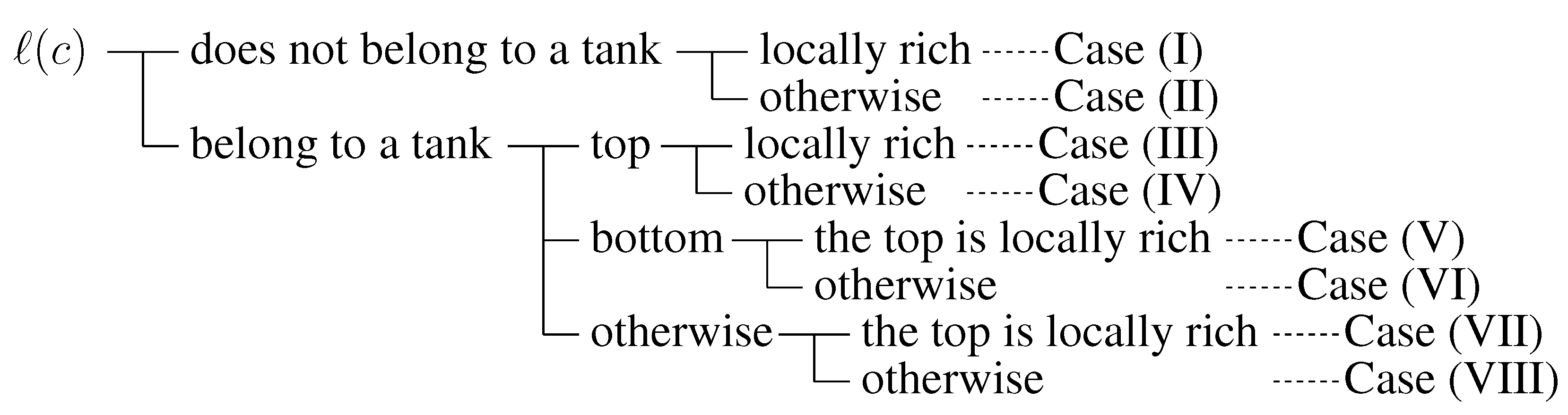
Next, we describe executions of
Extended-Lazy for deletions. Similarly as
Sec. 3.1., for a deletion
, there are eight cases depending on the status of level
as summarized in
Figure 7, each of which will be explained in the following.
Case (I): The case that does not belong to a tank and is locally rich. Remove c. If c is the rightmost dead vertex at , do nothing. Otherwise, use FreeTail() and receive a code of level . Then, using AppendLeft(), assign to the vertex to which c was assigned. Note that the vertex v which was the rightmost dead vertex of level becomes non-dead after the above operations, which may turn some dead vertices in the path from v to the root non-dead. As a result, an assignment may become non-semi-compact. If the semi-compactness is broken, we use the operation Repair, which will be explained later, to retrieve the semi-compactness. The cost of this case is either 1 or 0, and the number of locally rich levels decreases by one without considering the effect of Repair. (We later estimate these quantities considering the effect of Repair.)
Figure 7.
Execution of Extended-Lazy for a deletion .
Figure 7.
Execution of Extended-Lazy for a deletion .
Case (II): The case that does not belong to a tank and is not locally rich. Extended-Lazy behaves in exactly the same way as Case (I). Note that vertex v which was the rightmost dead vertex at level becomes non-dead after the above operations, but v is a right child because was not locally rich. Since the semi-compactness was satisfied before the execution, the vertex immediately left of v was (and is) dead, which implies that the parent and hence all ancestors of v are still dead. Thus, we do not need Repair in this case. It costs either 1 or 0, and the number of locally rich levels increases by one or remains unchanged because may become locally rich.
Case (III): The case that belongs to tank[], , and t is locally rich. First, remove c. Next, execute FreeTail(t) and receive the code of level b from tank[]. If c was assigned to the vertex immediately left of tank[] at t, do nothing. Otherwise, using FreeTail(t), receive a code of level t, and using AppendLeft(), assign to the vertex to which c was assigned. We then find a level to which we assign the code . Starting from level t, we see if the level contains at least one code, until we reach level . Let ℓ be the first such level. Then execute AppendRich(), which creates tank[]. If there is no such level ℓ between t and , execute AppendRich(). In this case, we may need Repair. Without considering the effect of Repair, it costs either 1 or 2. If it costs 1, the number of locally rich levels stays unchanged or decreases by one, and if it costs 2, the number of locally rich levels decreases by one.
Case (IV): The case that belongs to tank[], , and t is not locally rich. Extended-Lazy behaves in exactly the same way as Case (III). In this case, we do not need Repair by a similar observation as Case (II). It costs either 1 or 2, and the number of locally rich levels increases by one.
Case (V): The case that belongs to tank[], , and t is locally rich. First, remove c. If c was the code assigned to tank[], stop here; otherwise, do the following: Execute FreeTail(t) and receive the code of level b from tank[]. Then, using AppendLeft(), assign to the vertex to which c was assigned. In this case, we may need Repair because tank[b, t] becomes unassigned. The incurred cost is 1 or 0, and the number of locally rich levels decreases by one without considering the effect of Repair.
Case (VI): The case that belongs to tank[], , and t is not locally rich. Extended-Lazy behaves in exactly the same way as Case (V). In this case, we do not need Repair for the same reason as Case (II). The cost is 1 or 0, and the number of locally rich levels increases by one.
Case (VII): The case that belongs to tank[], , and t is locally rich. First, remove c. Next, execute FreeTail(t) and receive the code of level b from tank[]. If c was assigned to the rightmost assigned vertex at , do nothing. Otherwise, using FreeTail(), receive a code of level , and using AppendLeft(), assign to the vertex to which c was assigned. We then find a level to which we assign the request in the same way as Case (III). Starting from level , we see if the level contains at least one code, until we reach level . Let ℓ be the first such level. Then execute AppendRich(), which creates tank[]. If there is no such level ℓ between and , execute AppendRich(). In this case, we may need Repair. Without considering the effect of Repair, it costs either 1 or 2. If it costs 1, the number of locally rich levels is unchanged or decreases by one, and if it costs 2, the number of locally rich levels decreases by one.
Case (VIII): The case that belongs to tank[], , and t is not locally rich. Extended-Lazy behaves in exactly the same way as Case (VII). In this case, we do not need Repair for the same reason as Case (IV). The cost is 1 or 2. The number of locally rich levels increases by one or two when the cost is 1, and by one when the cost is 2.
Recall that after executing Cases (I), (III), (V), or (VII), the OVSF code tree may not satisfy semi-compactness. In such a case, however, there is only one level that breaks the conditions of semi-compactness, and furthermore, there is only one broken condition, namely, either (ii) or (v). If (ii) is broken at level
ℓ, level
ℓ consists of, from left to right, a sequence of unassigned dead vertices up to some point, one non-dead vertex
v, a sequence of (at least one) assigned dead vertices, and a sequence of non-dead vertices. Note that, if
ℓ is a bottom of a tank tank[
ℓ,
t], the last non-dead vertices include a leftmost level-
ℓ descendant of tank[
ℓ,
t] (which is non-dead by definition). This non-dead vertex
v was called a “hole” in [
6]. We also use the same terminology here, and call level
ℓ a
hole-level. If (v) is broken at level
ℓ,
ℓ is a bottom of tank[
ℓ,
t] and is rich. Furthermore, level
ℓ consists of, from the leftmost vertex, a sequence of one or more unassigned dead vertices, a sequence of one or more non-dead vertices, and then the leftmost level-
ℓ descendant of tank[
ℓ,
t]. We call level
ℓ a
rich-bottom-level. A level is called a
critical-level if it is a hole-level or a rich-bottom-level.
The idea of Repair is to resolve a critical-level one by one. When we remove a critical-level ℓ by Repair, it may create another critical-level. However, we can prove that there arises at most one new critical level, and its level is higher than ℓ. Hence we can obtain a semi-compact assignment by applying Repair at most h times.
We explain the operation
Repair. If
ℓ is a hole-level and
ℓ is not a bottom of a tank, then we execute FreeTail(
ℓ) so that we receive a code
c and execute AppendLeft(
), i.e., we release the code
c assigned to the rightmost assigned vertex at level
ℓ, and reassign
c to the hole to fill it. (See
Figure 8.) In this case, the cost of
Repair is 1. If
ℓ is locally rich, the number of locally rich levels decreases by one and at most one critical-level may appear, which means that we may need to apply
Repair once more. Otherwise, the number of locally rich levels increases by one and a critical-level does not appear. If
ℓ is a hole-level
Figure 8.
Repair for a hole-level ℓ which is not a bottom of a tank.
Figure 8.
Repair for a hole-level ℓ which is not a bottom of a tank.
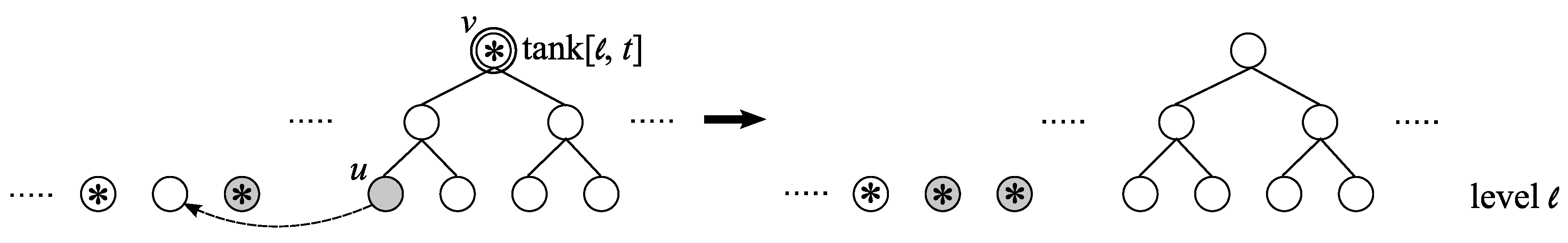
and
ℓ is a bottom of a tank
v(=tank[
ℓ,
t]), then there is a vertex
u that is the leftmost level-
ℓ descendant of
v. Recall that the code virtually assigned to
v is actually a code for level
ℓ and is assigned to
u. We release this code
c using FreeTail(
t) and perform AppendLeft(
). (See
Figure 9.) In this case, the cost of
Repair is 1. If
t is locally rich, the number of locally rich levels decreases by one and at most one critical-level may appear, which means that we may need to apply
Repair once more. Otherwise, the number of locally rich levels increases by one and a critical-level does not appear.
Figure 9.
Repair for a hole-level ℓ which is a bottom of a tank v.
Figure 9.
Repair for a hole-level ℓ which is a bottom of a tank v.
Finally, if
ℓ is a rich-bottom-level, then we will do the same operation, namely, release the code
c from the tank, and execute AppendLeft(
). (See
Figure 10.) In this case, the cost of
Repair is 1. If
t is locally rich, the number of locally rich levels decreases by one and at most one critical-level may appear, which means that we may need to apply
Repair once more. Otherwise, the number of locally rich levels increases by one and a critical-level does not appear.
Figure 10.
Repair for a rich-bottom-level ℓ.
Figure 10.
Repair for a rich-bottom-level ℓ.
Lemma 3. Extended-Lazy preserves the semi-compactness on deletions.
Proof. Similarly as Lemma 2, we will check that the five conditions (i) through (v) of semi-compactness are preserved for each application of Cases (II), (IV), (VI), and (VIII). For Cases (I), (III), (V), and (VII), at most one critical-level may appear but the five conditions (i) through (v) must be preserved at all other levels. We also need to verify these facts for Repair, but this can be done similarly, and we will omit it here. It is relatively easy to show that condition (i) is preserved because removing codes, and applying AppendRich, AppendPoor, FreeTail, and AppendLeft preserve the orthogonality. So, in the following, we will check conditions (ii) through (v). Similarly as Cases (1) and (3) in the proof of Lemma 2, we check conditions for each group of levels.
Case (I):
| : | Nothing changes. Thus, all the conditions remain satisfied. |
| : | Only the rightmost assigned vertex turns unassigned by removing c, and applying FreeTail() and AppendLeft(). Therefore, condition (ii) remains satisfied. Since does not belong to any tank, conditions (iii), (iv), and (v) also remain satisfied. |
| : | Conditions (iii) and (iv) remain satisfied because no tank is removed or created. In the following, we show that there is at most one level that breaks the conditions (ii) or (v). Since the rightmost dead vertex v at level turns non-dead and v is the left child of its parent , turns from dead to non-dead. Also, if was the rightmost dead vertex at level and is the left child of its parent , turns from dead to non-dead. Otherwise, remains dead. In this way, we can apply the same argument to the upper levels. Then there is a level such that one vertex turns from dead to non-dead at each level from to , and nothing changes at levels or higher. Clearly, levels or higher do not break the conditions. Also, we can see that both conditions (ii) and (v) are satisfied at any level in as follows: Consider a level and suppose that at level ℓ turns from dead to non-dead. Condition (ii) is satisfied at ℓ because was the rightmost dead vertex at ℓ. Condition (v) is also satisfied for the following reason: was the rightmost dead vertex at ℓ and is the left child of its parent, so ℓ was locally rich. Since condition (v) was satisfied before the application of Case (I), ℓ must not belong to a tank. So, the conditions can be broken only at . Let be the vertex at that turns from dead to non-dead. Note that if (ii) is broken, was not the rightmost dead vertex, while if (v) is broken, was the rightmost dead vertex (since turns from poor to rich), namely, cannot break both (ii) and (v). This completes the proof. |
Case (II):
| : | All the conditions are satisfied by the same argument as Case (I). |
| : | Since v is a right child and its sibling remains dead, the parent of v remains dead. So, the statuses of all vertices remain the same. Thus, all the conditions remain satisfied. |
Case (III):
| : | Nothing changes and so all the conditions remain satisfied. |
| : | The tank tank[] is removed and tank[] is created. However, nothing changes except for the tanks. Thus, all the conditions remain satisfied. |
| ℓ: | If , tank[] is moved to the vertex immediately left of tank[]. Thus, conditions (ii), (iii), and (v) remain satisfied. Also, condition (iv) remains satisfied, because there is at least one assigned vertex except for tank[] at t. If , is assigned to the vertex to the right of the rightmost dead vertex which is also assigned and tank[] is created. Hence, conditions (ii) and (iv) remain satisfied. Also, condition (iii) remains satisfied because tank[] is removed and tank[] is created. Since ℓ is the top of tank[], condition (v) also remain satisfied |
| : | Only tank[] is removed. Therefore, all the conditions remain satisfied. |
| t: | We have already proven above the case of . Otherwise, tank[] is removed and the rightmost assigned vertex v turns unassigned. Since levels [) were poor, there was an assigned ancestor of the leftmost non-dead vertices at levels [). The assigned ancestor was v because there were no assigned vertices at levels (). Hence, v remains dead. Condition (ii) remains satisfied because only the rightmost dead vertex turns non-dead. Conditions (iii), (iv), and (v) also remain satisfied because tank[] is removed. |
| : | We can use the same argument as the proof for levels (] of Case (I). |
Case (IV):
| : | All the conditions remain satisfied by the same discussion as Case (III). |
| : | The parent of tank[] remains dead because tank[] is a right child and its sibling remains dead as we proved in the proof of Case (III). So, the statuses of all vertices remain the same. Thus, all the conditions remain satisfied. |
Case (V):
| : | Nothing changes and so all the conditions remain satisfied. |
| : | Only tank[] is removed and all the conditions remain satisfied. |
| t: | The tank tank[] is removed and the rightmost dead vertex, which was tank[], turns non-dead. Condition (ii) remains satisfied because only the rightmost dead vertex turns non-dead. Also conditions (iii), (iv), and (v) remain satisfied because tank[] is removed. |
| : | We can use the same argument as the proof for level (] of Case (I). |
Case (VI):
| : | All the conditions remain satisfied by the same discussion as Case (V). |
| : | Since tank[] is a right child and its sibling remains dead, the parent of tank[] remains dead. So, the statuses of all vertices remain the same. Thus, all the conditions remain satisfied. |
Case (VII):
| : | Nothing changes and so all the conditions remain satisfied. |
| : | We can use the same argument as the proof for levels ] of Case (III). |
| : | Only tank[] is removed and all the conditions remain satisfied. |
| t: | The tank tank[] is removed and the rightmost dead vertex, which was tank[], turns non-dead. Condition (ii) remains satisfied because only the rightmost dead vertex turns non-dead. Also conditions (iii), (iv), and (v) remain satisfied because tank[] is removed. |
| : | We can do the same argument as the proof for level (] of Case (I). |
Case (VIII):
| : | All the conditions remain satisfied by the same discussion as Case (VII). |
| : | The statuses of all vertices remain the same by the same discussion as Case (VI). ☐ |


