CADrx for GBM Brain Tumors: Predicting Treatment Response from Changes in Diffusion-Weighted MRI

Abstract

The goal of this study was to develop a computer-aided therapeutic response (CADrx) system for early prediction of drug treatment response for glioblastoma multiforme (GBM) brain tumors with diffusion weighted (DW) MR images. In conventional Macdonald assessment, tumor response is assessed nine weeks or more post-treatment. However, we will investigate the ability of DW-MRI to assess response earlier, at five weeks post treatment. The apparent diffusion coefficient (ADC) map, calculated from DW images, has been shown to reveal changes in the tumor’s microenvironment preceding morphologic tumor changes. ADC values in treated brain tumors could theoretically both increase due to the cell kill (and thus reduced cell density) and decrease due to inhibition of edema. In this study, we investigated the effectiveness of features that quantify changes from pre- and post-treatment tumor ADC histograms to detect treatment response. There are three parts to this study: first, tumor regions were segmented on T1w contrast enhanced images by Otsu’s thresholding method, and mapped from T1w images onto ADC images by a 3D region of interest (ROI) mapping tool using DICOM header information; second, ADC histograms of the tumor region were extracted from both pre- and five weeks post-treatment scans, and fitted by a two-component Gaussian mixture model (GMM). The GMM features as well as standard histogram-based features were extracted. Finally, supervised machine learning techniques were applied for classification of responders or non-responders. The approach was evaluated with a dataset of 85 patients with GBM under chemotherapy, in which 39 responded and 46 did not, based on tumor volume reduction. We compared adaBoost, random forest and support vector machine classification algorithms, using ten-fold cross validation, resulting in the best accuracy of 69.41% and the corresponding area under the curve (Az) of 0.70.

1. Introduction

Computer aided diagnosis (CADx) can be defined as a diagnosis that is made by a radiologist who uses the output from a computerized analysis of medical images as a “second opinion” in both detecting lesions and making diagnostic decisions [1]. One aim of the typical CADx system is to extract and analyze the characteristics of benign and malignant lesions in an objective manner to aid the radiologist. Here, the “diagnostic” decision relates to treatment response and early classification of drug responders versus non-responders, and we name our proposed system as computer-aided therapeutic response (CADrx) system.

Glioblastoma multiforme (GBM) is the most aggressive and lethal primary brain tumor in human. Anti-angiogenesis drugs are increasingly being explored in clinical trials as therapeutic options. In a phase II in vivo clinical trial, the conventional way to assess treatment response is the tumor size change after chemotherapy or radiotherapy based on Macdonald criteria and evaluated on T1-weighted contrast enhanced (T1wCE) MR images. However, efficacy can only be evaluated at least 8–10 weeks after treatment.

Diffusion weighted magnetic resonance imaging (DW-MRI) has the potential to work as a surrogate biomarker to reveal changes in the tumor microenvironment that precede morphologic tumor changes [2]. DW-MRI depends on the microscopic mobility of water. This mobility, classically called Brownian motion, is due to thermal agitation and is highly influenced by the cellular environment of water. Because water diffusion is strongly affected by molecular viscosity and membrane permeability between intra- and extracellular compartments, DW-MRI can be used to characterize highly cellular regions of tumors versus acellular regions. Treatment response detection can be manifested as a change in tumor cellularity, which may precede tumor size changes. Thus, findings on DW-MRI could be an early sign of biologic changes. [3]

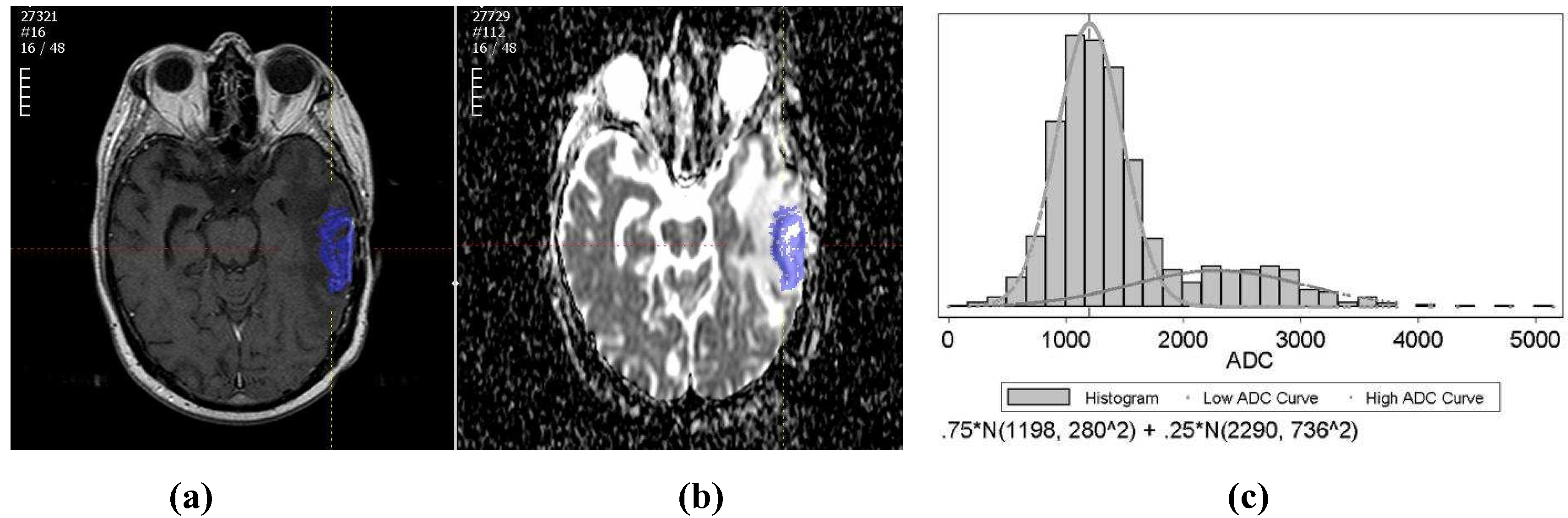
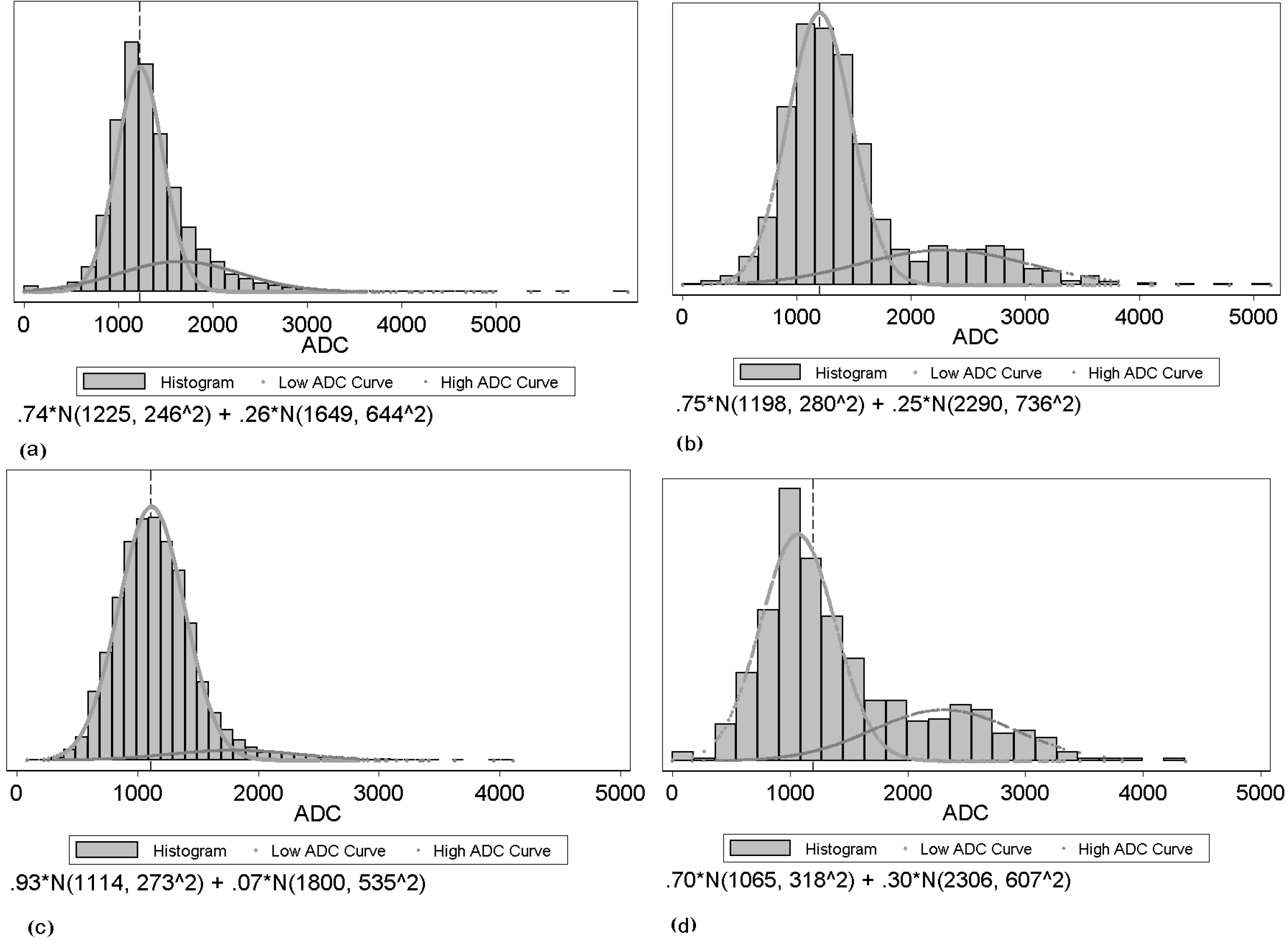
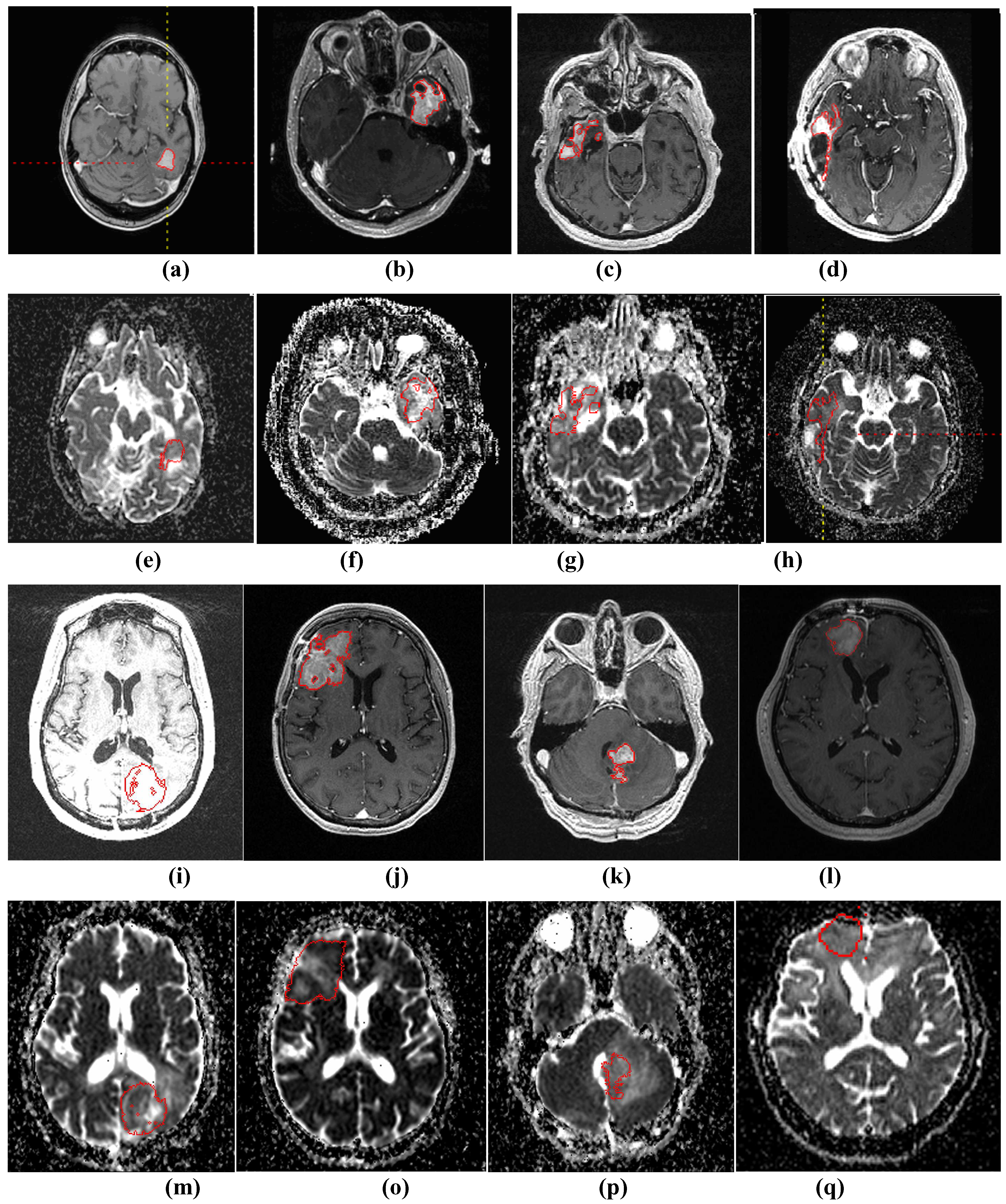
The purpose of this study is to use apparent diffusion coefficient (ADC), derived from DW-MR images, for early prediction of the tumor volume change on a later scan. There are two main parts to this computer-aided treatment response evaluation system. First, a semi-automated segmentation algorithm is applied to segment the GBM brain tumors on T1wCE images. Then, the tumor ROI is mapped onto derived ADC maps and the histogram of tumor ADC values will be extracted for automatic treatment response prediction.

Computer-aided detection and segmentation of GBM brain tumors is a challenging problem and in Table 1 we present a concise review of the prior art in automatic tumor segmentation. Fuzzy clustering and knowledge-based analysis are popular methods explored by the early pioneers [4,5,6]. Voxel-based classification method using statistical pattern classification techniques are explored by others [7,8,9,10,11,12,13,14,15]. Most of the studies above use multiple MRI sequences (T1w, T2w, proton density weighted, and Flair) for the automatic tumor and edema detection and segmentation. Liu et al. [16] developed an interactive system adapting the fuzzy connectedness using multiple MRI sequences. Dube et al. [17,18] used texture features and segmentation by the weighted aggregation (SWA) method for the GBM tumor segmentation on T1wCE images which is similar to part of our study. In our study, we developed semi-automated method to segment tumors on T1wCE images; in addition, we mapped the tumor contours onto ADC maps.

Table 1. Summary of related methods in brain tumor segmentation. The type abbreviations are NC: Nasopharyngeal carcinoma; MNG: Meningiomas; MG - malignant gliomas; MS – multiple sclerosis.

Authors	Technique	Type	Image sequences	# of tumors
Liu et al. [16]	Semi-automated fuzzy clustering	GBM	T1w, T1w+c, Flair	5
Philips et al. [4]	Fuzzy clustering	GBM	PD,T2w, T1w+c	1
Clark et al. [5]	Fuzzy clustering and knowledge-based analysis	GBM	PD,T2w, T1w+c	7
Fletcher-Heath et al. [6]	Fuzzy clustering and knowledge-based analysis	Brain tumor	PD,T2w, T1w with no contrast	4
Prastawa et al. [7]	Learn distribution of normal tissues/outlier detection as tumors	Brain tumors	T2w, T1w (with or without contrast)	3
Kaus et al. [8]	Adaptive template -moderate technique with atlas prior	LGG/MG	T1w+c, sagittal view	20
Lee et al. [11]	Conditional random field and support vector machine	Brain tumors	T1w, T1w+c, T2w	7
Ho et al. [9]	3D level set	GBM	T1w+c, T1w, T2w	3
Vinitski et al. [10]	k-nearest neighbor	MS and MG	PD, T2w, T1w, magnetization transfer	9
Zhu & Yan et al. [12]	Hopfield neural network	Brain tumors	NA	2
Zhang et al. [13]	Support vector machine	NC	T1w, T1w+c	9
Corso et al. [15]	SWA-segmentation by weighted aggregation.	GBM	T2w, T1w, T1w+c, Flair	20
Dube et al. [17]	SWA with texture features	GBM	T1w+c	NA
Nie et al. [14]	Spatial accuracy-weighted hidden Markov field and EM to solve the problem of high and low resolution problem	Gliomas	High:T1w, T1w+c Low:T2w, Flair	15

Table 1. Summary of related methods in brain tumor segmentation. The type abbreviations are NC: Nasopharyngeal carcinoma; MNG: Meningiomas; MG - malignant gliomas; MS – multiple sclerosis.

Authors	Technique	Type	Image sequences	# of tumors
Liu et al. [16]	Semi-automated fuzzy clustering	GBM	T1w, T1w+c, Flair	5
Philips et al. [4]	Fuzzy clustering	GBM	PD,T2w, T1w+c	1
Clark et al. [5]	Fuzzy clustering and knowledge-based analysis	GBM	PD,T2w, T1w+c	7
Fletcher-Heath et al. [6]	Fuzzy clustering and knowledge-based analysis	Brain tumor	PD,T2w, T1w with no contrast	4
Prastawa et al. [7]	Learn distribution of normal tissues/outlier detection as tumors	Brain tumors	T2w, T1w (with or without contrast)	3
Kaus et al. [8]	Adaptive template -moderate technique with atlas prior	LGG/MG	T1w+c, sagittal view	20
Lee et al. [11]	Conditional random field and support vector machine	Brain tumors	T1w, T1w+c, T2w	7
Ho et al. [9]	3D level set	GBM	T1w+c, T1w, T2w	3
Vinitski et al. [10]	k-nearest neighbor	MS and MG	PD, T2w, T1w, magnetization transfer	9
Zhu & Yan et al. [12]	Hopfield neural network	Brain tumors	NA	2
Zhang et al. [13]	Support vector machine	NC	T1w, T1w+c	9
Corso et al. [15]	SWA-segmentation by weighted aggregation.	GBM	T2w, T1w, T1w+c, Flair	20
Dube et al. [17]	SWA with texture features	GBM	T1w+c	NA
Nie et al. [14]	Spatial accuracy-weighted hidden Markov field and EM to solve the problem of high and low resolution problem	Gliomas	High:T1w, T1w+c Low:T2w, Flair	15

Computer-aided diagnosis (CADx) in GBM brain tumor is an active research area, and many promising MR methods have been developed for detecting and characterizing cancer, its treatments and adverse effects, e.g. T1-weighted MR, T2-weighted MR, MR spectroscopy, perfusion-weighted MR, and diffusion-weighted MR. In our study, we focused on T1-weighted and DW-MRI. Tumor size change on T1w images is the only imaging biomarker that is accepted by the FDA as a surrogate endpoint of clinical outcome after chemotherapy and radiotherapy for phase III trials [19]. Diffusion MRI has been explored as early detection of human GBM brain tumor treatment response early therapeutic responses before the tumor size changes. Table 2 presents a review of the recent studies that used DWI for GBM early prediction of treatment response. Ross et al reported ADC value increase significantly in effective therapeutic intervention in pre-clinical studies and presented two patients to support this hypothesis in a preliminary clinical study [2,20]. Mardor et al. [21] applied both low and high b-value and used mean ADC and diffusion index for treatment response evaluation. Moffat et al calculated voxel-by-voxel tumor ADC value changes over time and displayed it as a functional diffusion map for correlation with clinical response [22,23]. They reported that the number of voxels with increased ADC is related to treatment efficacy. Our previous work [24] showed promising results for using ADC histogram analysis, and we explored a more sophisticated classifier and designed experiments to show the advantages of the two-component histogram modeling.

Table 2. Summary of related methods in GBM tumor treatment response using DWI.

Authors	# Of Patients
Chenevert et al. [20]	2
Ross et al. [2]	2
Mardor et al. [21]	10
Moffat et al. [22]	20
Hamstra et al. [23]	34

Table 2. Summary of related methods in GBM tumor treatment response using DWI.

Authors	# Of Patients
Chenevert et al. [20]	2
Ross et al. [2]	2
Mardor et al. [21]	10
Moffat et al. [22]	20
Hamstra et al. [23]	34

Machine learning and statistical pattern recognition have great contributions to the biomedical community because they can improve the sensitivity and/or specificity of detection and diagnosis of disease, while at the same time increasing objectivity of the decision-making process [26]. The need for machine learning is perhaps greater than ever given the dramatic increase in medical data being collected, new detection, and diagnostic modalities being developed as well as the complexity of the data types and importance of multimodal analysis. In all of these cases, machine learning can provide new tools for interpreting the high-dimensional and complex datasets with which the clinician is confronted [26]. In our study, we explored three different classification methods: AdaBoost, random forest, and support vector machine.

The AdaBoost algorithm, introduced by Freund and Schapire [27], is an iterative algorithm that can boost weak classifiers into a strong classifier and improve the final accuracy. In each iteration, a feature is working as a weak classifier and the best feature is selected to minimize the average training error. Afterwards, the weights on training samples are redistributed in such a way that the weight of accurately classified samples will be reduced while the weight of ill classified samples is raised. Therefore, AdaBoost focuses on the most “difficult” ones [28]. The final classifier aggregates the selected weak classifier from each iteration, and the weight for each weak classifier depends on its error rate. However, AdaBoost can be sensitive to noise and may introduce the overfitting problem.

Random forests (RF) is a classifier that combines many decision trees [29]. Each tree depends on values of a random vector sampled independently and with equal distribution. Each tree casts a unit vote for the most popular case at input, and random forests outputs the class that is the mode of the classes output by individual trees. Breiman suggests the generalization error for forests converges to a limit as the number of trees in the forest becomes large [30]. The error of a forest of tree classifiers depends on the strength of the individual trees in the forest and the correlation between them. Using a random selection of features to split each node yields error rates that compare favorably to Adaboost but are more robust with respect to noise.

Support vector machines (SVMs) are a set of related supervised learning methods used for classification and regression [31,32]. Viewing input data as two sets of vectors in an n-dimensional space, an SVM will construct a separating hyperplane in that space, one which maximizes the margin between the two data sets. To calculate the margin, two parallel hyperplanes are constructed, one on each side of the separating hyperplane, which are "pushed up against" the two data sets. Intuitively, a good separation is achieved by the hyperplane that has the largest distance to the neighboring data points of both classes, since in general the larger the margin the lower the generalization error of the classifier [33]. SVM have been reported to work well for pharmaceutical data analysis [34].

There are two main challenges in this work. One challenge is the two competing effects in ADC changes after treatment. In general, water movement inside cells is more restricted than outside. Thus, increased cell density tends to lower ADC values, whereas increased edema (more interstitial water) results in higher ADC values. Therefore, theoretically, ADC values in treated brain tumors could not only increase due to the cell kill (and thus reduced cell density), but also decrease due to inhibition of edema. None of the listed studies above have specified the separate effects. Thus, we applied a two-component model to fit the tumor ADC histogram [25]. The other challenge is that it is difficult to directly identify GBM brain tumors on ADC maps. We developed a semi-automated framework to achieve that goal.

There are several contributions in this work. First, we developed a computer-aided method to semi-automatically identify tumors on ADC maps. Second, we explored the changes of different statistical features of the whole tumor ADC histogram. Moreover, we applied a two-component Gaussian mixture modeling to fit the tumor ADC histogram to overcome the two competing effects. Next, we used earth mover’s distance (EMD) to directly measure the distance between the pre- and post-treatment tumor ADC histograms. Finally, we introduced machine learning technique to do feature selection and classification to classify responders and non-responders.

This paper is organized as follows: Section 2 describes the image acquisition and patient group, Section 3 describes the semi-automated identification of GBM tumors on ADC maps, and Section 4 describes the histogram feature extraction and classification. The Result Section reports the performance of the tumor mapping on ADC maps, and the results of our comparative study for three different classifiers. The final section offers a discussion of the experimental results as well as the future work.

2. Image Acquisition

2.1. Patient cohort

A total of 85 patients with GBM treated by anti-angiogenesis drugs were included in our preliminary study from our research database. Images in this database were acquired as part of multicenter GBM treatment trial. Tumors were diagnosed by board-certified radiologists as responders or non-responders to drugs based on Macdonald criteria from follow-up scans (8–10 weeks after baseline). The Macdonald criteria define tumor response by use of tumor size change, steroids, and neurological functions. There are four ‘response’ categories: complete response (CR): disappearance of enhancing tumors, off steroids, and neurologically stable or improved. Partial response (PR): >50% reduction in size of enhancing tumor, steroids stable or reduced, neurologically stable or improved. Progressive disease (PD): >25% increase in size of enhancing tumor or any new tumor, or neurologically worse, and steroids stable or increased. Stable disease (SD): all other situations. In our study, we used tumor volume to evaluate tumor sizes. More than 50% increase in volume is considered to be the PD based on the neuro-radiologist’s suggestion [44]. Since GBM is a rapidly progressing disease, we classified PD as non-responders and CR, PR and SD as responders. As a result, 39 were responders and 46 were non-responders. The DW-MRI scans were performed 5–7 weeks apart between baseline and follow-up scans.

The patients in this study were pooled from six medical sites scanned on 9 different scanner models (GE/Siemens) including both 1.5 T and 3 T scanners. The imaging protocol for T1wCE is 3D volume in the axial plane with flip angle-spoiled gradient echo sequence (FSPGR) or magnetization-prepared rapid gradient-echo (MP-RAGE) sequence, 1–5 mm slice thickness, 0.9375 mm by 0.9375 mm pixel size, and 256 × 256 in-plane resolution. The imaging protocol for the DW images is either DWI or different tensor imaging (DTI), 700–1,000 s/mm² for b-value, 3–30 for the number of diffusion sensitization probing directions, 5–7 mm slice thickness, 1.797mm by 1.797 mm pixel size, and 256 × 256 or 128 × 128 in-plane resolution.

We developed a quality assurance technique to evaluate the consistency of ADC measurements from multiple scanners and multiple visits by use of ROI analysis with normal appearing white matter [35]. Our study [35] showed that there is no significant difference in ADC measurement among the different scanner models used. For the between-visit reproducibility, ADC measurement was found to be reproducible with consistent image protocols.

2.2. ADC map derivation

All ADC maps were calculated from DW-MR images with the same in-house software using a two-point method as shown in the following equation:

ADC = -ln[S(b)/S(0)]/b

(1)

with b being the diffusion sensitivity factor ranging between 700 and 1,000 s/mm², S(0) and S(b) being the image intensity when b = 0 and b = 700 – 1,000 s/mm². For DWI images, we calculated ADC maps from DW images by equation (1). For DTI, we calculated ADC for each orientation and averaged them as the final ADC map. Figure 1(b) shows an example of a derived brain ADC map.

Figure 1. (a) An example of the tumor segmented on a T1wCE image; (b) An example of the tumor ROI mapped from T1wCE to ADC map; (c) An example of the tumor ADC histogram fitted by two-component Gaussian mixtures.

Figure 1. (a) An example of the tumor segmented on a T1wCE image; (b) An example of the tumor ROI mapped from T1wCE to ADC map; (c) An example of the tumor ADC histogram fitted by two-component Gaussian mixtures.

3. Semi-Automated Image Analysis on ADC Maps

All patients were scanned by both T1wCE MR images and DW-MR images. Since it is difficult to segment tumors accurately on derived ADC maps, we segmented tumors on T1wCE images first, and then mapped the tumor contours onto the corresponding ADC maps.

3.1. Tumor segmentation on T1wCE MR images

All tumors were segmented on T1wCE images via a semi-automated method using the Otsu’s thresholding algorithm [36] and seeded region growing [37]. First, radiologists drew a line from inside of the tumor to the outside of the tumor on the approximate center slice of the tumor. Then intensity values along the line were collected to form a bimodal histogram, and the Ostu’s thresholding method was used to find the optimal thresholding value. Afterwards, a 3D seeded region growing was applied to obtain the segmentation results in the whole volume. Threshold-based segmentation methods are a standard approach to calculation of tumor volume.

The concept behind the Otsu’s thresholding method [36] is to find the threshold that minimizes the weighted within-class variation ${\sigma }_w^2$ as in equation (2), considering the two-class segmentation into object and background:

(2)

with q(t) as the class probability, μ_c(t) as class mean, σ_c(t) as class variance, c = 1,2 as two different classes, t is variable for the intensity value, and P(.) is the probability density function. Given an initial class mean and variance, the algorithm will do an exhaustive search by altering the thresholding value to find the optimal thresholding value.

Afterwards, seeded region growing [37] using the optimal thresholding value was applied to get the tumor contours in the 3D volume. Radiologists reviewed the results and made manual corrections when necessary. Figure 1(A) shows an example of a segmented tumor on a T1wCE image.

3.2. Tumor mapping from T1wCE images to ADC maps

It is difficult for radiologists to directly delineate the tumor contours on ADC maps, and the scanner-provided T1w images and the derived ADC maps are not inherently co-registered, because they have different slice thickness, different field of view (FOV), and different image resolutions. Therefore, a 3D ROI mapping tool was developed to map the tumor ROIs from T1wCE images onto ADC maps based on the scanner geometry. Compared to the co-registration technique, the mapping tool only transformed voxels within the tumor ROI rather than the whole image volume; thus it was more computationally efficient. However, the mapping tool could not correct for patient motion; thus a board-certified radiologist was required to visually check the mapped results and perform manual corrections when necessary.

The mapping tool used an affine transformation with the parameters extracted from the DICOM header based on physical locations. Equation 3 shows the way to calculate the 3D physical location voxelwise. Δ_i,j.k is the physical voxel size read from the tag “pixel spacing” and calculated from “slice location”; X_x,y,z, Y_x,y,z is image orientation read from the tag “image orientation” which specifies the orientation of the image frame rows and columns, Z_x,y,z is the z-direction orientation calculated from X_x,y,z, Y_x,y,z, S_x,y,z is read from the tag “patient position” which specifies the physical location of the patient’s anterior-left-upper corner; i, j, k are voxel index; and P_x,y,z are the calculated physical location of the voxel in millimeters. The transformation matrices are calculated for both source and target ROI respectively. For each voxel in the source ROI, the physical location is first calculated, and then the inverse operation is performed to calculate the corresponding voxel coordinates of the target ROI. Finally, radiologists visually check the contours on ADC maps and manually correct the tumor contours on ADC when necessary. Figure 1(B) shows an example of the mapped tumor ROI on the ADC map from the T1wCE image.

     Equation 3. The physical location calculation of a voxel (i,j,k).

4. Feature Extraction and Classification

The differences between the features extracted from pre- and post-treatment tumor ADC histograms are used as the input to a tumor response classifier.

4.1. Observations

Figure 2 shows examples of tumor ADC histograms for both pre-and post-treatment with responders and non-responders. The upper histogram shows the ADC value distribution before the drug treatment, while the lower one shows the ADC value distribution after the drug treatment. On the left is an example of a volumetrically responding tumor, while on the right is an example of a non-responding tumor. From the figure, we observe that not only the location but also the shape of the responder’s histogram changes after treatment. The two Gaussian mixture components change as well.

4.2. General histogram features

Different statistical features from tumor ADC histograms were extracted. According to clinical studies, the ADC value should change after treatment. In our data set, we observed that the histograms exhibit change not only in location, but also in shape. Therefore, we introduced the extraction of different ADC histograms features and explored changes in their pattern. The features are: mean, standard deviation, skewness, kurtosis, median, IQR (interquartile range), 25% percentile, and 75% percentile.

Figure 2. Examples of histograms from two tumors and two time points: (a), (c): example of a responding tumor for pre- and post-treatment respectively; (b), (d): example of a non-responding tumor for pre- and post-treatment respectively.

Figure 2. Examples of histograms from two tumors and two time points: (a), (c): example of a responding tumor for pre- and post-treatment respectively; (b), (d): example of a non-responding tumor for pre- and post-treatment respectively.

4.3. Features from GMM

Two-component Gaussian mixture modeling was applied to each tumor ADC histogram and the two-component features were extracted. Due to the competing effects of tumor cell density and edema, we made the assumption that the obtained tumor ADC histogram was composed of two components relating to tumor cellularity and edema. We assumed that the component with lower peak is influenced by tumor cellularity, and the component with higher peak by edema effects. We used a two component GMM as shown in Equation 3 to fit the ADC histogram for both baseline and follow-up scans and applied EM algorithm to estimate GMM parameters, with x as the intensity values, a_i as the weight of the components, μ_i and σ_i as the Gaussian parameters.

(4)

The EM algorithm can be used to estimate the parameters of a parametric mixture model distribution: the weight of the components a_i, the Gaussian parameters μ_i, and σ_i. It is an iterative algorithm with two steps: an expectation step (E-step) and a maximization step (M-step).

In the E-step, with the current parameter estimates of the mixture components, the algorithm calculates the expectation values for the membership variables of all data points. In the (m+1) iteration, the expectation is:

(5)

In M-step, the algorithm maximizes the expectation value and updates the corresponding parameters. The following solutions can be developed:

(6)

The features we obtained from the GMM-EM were named as lower peak mean (LPM), lower peak variance (LPV), lower peak proportion (LPP), higher peak mean (HPM), higher peak variance (HPV) and higher peak proportion (HPP). Figure 2 shows examples of tumor ADC histograms fitted by GMM with low ADC and high ADC curves overlaid.

Combining GMM features with the statistical features, we obtained 14-dimensional feature vectors for both pre- and post-treatment tumor histograms. Afterwards, we calculated the rate of change between the pre- and the post-treatment tumor histogram. Therefore, we had a 14-dimensional vector as the difference feature vector.

4.4. Earth Mover’s Distance

Finally, we applied the earth mover's distance (EMD) [38,39] as a metric to directly evaluate the distance between the pre- and post-treatment tumor ADC histograms. Informally, if the histograms are interpreted as two different ways of piling up a certain amount of dirt over the region D, the EMD is the minimum cost of turning one pile into the other; where the cost is assumed to be amount of dirt moved times the distance by which is moved. The calculated EMD value was appended as the 15th element in the difference feature vector. The calculated 15-dimensional vector was the input feature vector for classification.

4.5. Classification

In this study for classification, we investigated three classification techniques with different characteristics: AdaBoost, random forests (RF) and support vector machine (SVM). We employed three classifiers to avoid biasing the results by selection of a single classification method. The reason we choose them is that the first two classifiers both include a feature selection mechanism. By applying these two classification techniques, we are seeking the best features that would separate responders from non-responders. SVM is reported to outperform several of the most frequently used machine learning techniques in structure–activity relationship (SAR) analysis. [34] In this study, all classifiers were implemented in the open source data mining software Weka [41]. Their performance was evaluated using 10-fold cross validation method.

Three experiments were performed. First, the conventional method of using mean ADC for treatment response classification was applied [2]. Second, the AdaBoost, RF classifier, and SVM were applied to the difference feature vectors of general statistical histogram features without GMM features, and results from the three classifiers were compared. Finally, the three classifiers were applied using all statistical features including the GMM features, and the results were compared, and the results of accuracies from different classification techniques were compared with conventional method of ADC mean changes by the test of proportion.

5. Results

5.1. Segmentation Performance

Figure 3 shows four examples of segmentation on T1wCE images and the mapped results on the derived ADC maps.

For quantitative evaluation of the tumor segmentation mapping results, we randomly selected 31 subjects’ baseline data. The 31 tumors are from an ADC mapping database, 20 of which have different image resolutions between the T1wCE and ADC images in all three dimensions and 11 of which have exactly the same 3D image resolution in both modalities. We calculated the overlap ratio between the mapped ROI generated automatically by the tool and an ROI corrected by a neuro-radiologist. The overlap ratio (OR) is defined by Equation 6, where A and B are two tumor ROIs and size(.) is the number of voxels in that ROI.

(7)

The results are shown in Table 3 with 20 out of 31 ROIs (64.5%) have an overlap ratio over 90%.

Table 3. Distribution of overlap ratios.

Overlap ratio	100%	95~100%	90~95%	80~90%	60~80%	0~60%
Number of patients	10	7	3	2	5	4

Table 3. Distribution of overlap ratios.

Overlap ratio	100%	95~100%	90~95%	80~90%	60~80%	0~60%
Number of patients	10	7	3	2	5	4

Figure 3. (a)-(d) and (i)-(l) show four examples of tumor segmentations on T1wCE images; (e)-(h) and (m)-(p) show the corresponding mapped tumor contours on ADC maps.

Figure 3. (a)-(d) and (i)-(l) show four examples of tumor segmentations on T1wCE images; (e)-(h) and (m)-(p) show the corresponding mapped tumor contours on ADC maps.

5.2. Classification Performance

Using the conventional method of mean ADC change (subjects with a mean ADC increase classified as responders and those with an ADC decrease as non-responders) [2,20], the accuracy is 29.4% (25/85), with a sensitivity of 17.95% and a specificity of 60.87% (see Table 4).

Table 4. Performance of the conventional mean ADC classification method.

Classifier	Sensitivity	Specificity	Accuracy	Az
Mean ADC change	17.95%	60.87%	29.4%	0.33

Table 4. Performance of the conventional mean ADC classification method.

Classifier	Sensitivity	Specificity	Accuracy	Az
Mean ADC change	17.95%	60.87%	29.4%	0.33

The experiment with AdaBoost involved 10 learning iterations. The RF classifier was composed of 10 trees, each of which is constructed considering five random features. The SVM classifier used non-linear polynomial kernels and normalized all features.

The results for the experiment using only the general histogram features without GMM are shown in Table 5 with sensitivity, specificity, accuracy and area under the ROC curve (Az). The ROC curves are shown in Figure 4. The curve using conventional mean ADC was plotted by varying the threshold of the mean ADC change used for the classification, while the curve using the three ML techniques were plotted by Weka. Weka plots the ROC curves by varying the threshold on the probability assigned to the positive class.

Table 5. Performance comparison among three classifiers without GMM features.

Classifier	Sensitivity	Specificity	Accuracy	Az
AdaBoost	45.45%	75%	63.53%*	0.61
Random forest	54.55%	73%	65.88%*	0.66
SVM	27.27%	92.3%	67.06%*	0.60

(*: All p-values <0.0001 comparing with accuracy of Table 4)

Table 5. Performance comparison among three classifiers without GMM features.

Classifier	Sensitivity	Specificity	Accuracy	Az
AdaBoost	45.45%	75%	63.53%*	0.61
Random forest	54.55%	73%	65.88%*	0.66
SVM	27.27%	92.3%	67.06%*	0.60

(*: All p-values <0.0001 comparing with accuracy of Table 4)

Figure 4. ROC curve for three classifiers without GMM features.

Figure 4. ROC curve for three classifiers without GMM features.

With GMM features added, the three classifiers with the same parameter setups were applied to the data. The results are shown in Table 6 with sensitivity, specificity, accuracy and area under the curve (Az) of the ROC curve. The ROC curves are shown in Figure 5.

Table 6. Performance comparison among three classifiers with GMM features.

Classifier	Sensitivity	Specificity	Accuracy	Az
AdaBoost	39.39%	80.77%	64.7%*	0.60
Random forest	51.52%	80.77%	69.41%*	0.70
SVM	27.27%	92.3%	67.06%*	0.60

(*: All p-values <0.0001 comparing with accuracy of Table 4)

Table 6. Performance comparison among three classifiers with GMM features.

Classifier	Sensitivity	Specificity	Accuracy	Az
AdaBoost	39.39%	80.77%	64.7%*	0.60
Random forest	51.52%	80.77%	69.41%*	0.70
SVM	27.27%	92.3%	67.06%*	0.60

(*: All p-values <0.0001 comparing with accuracy of Table 4)

Figure 5. ROC curve for three classifiers with GMM features.

Figure 5. ROC curve for three classifiers with GMM features.

6. Discussion

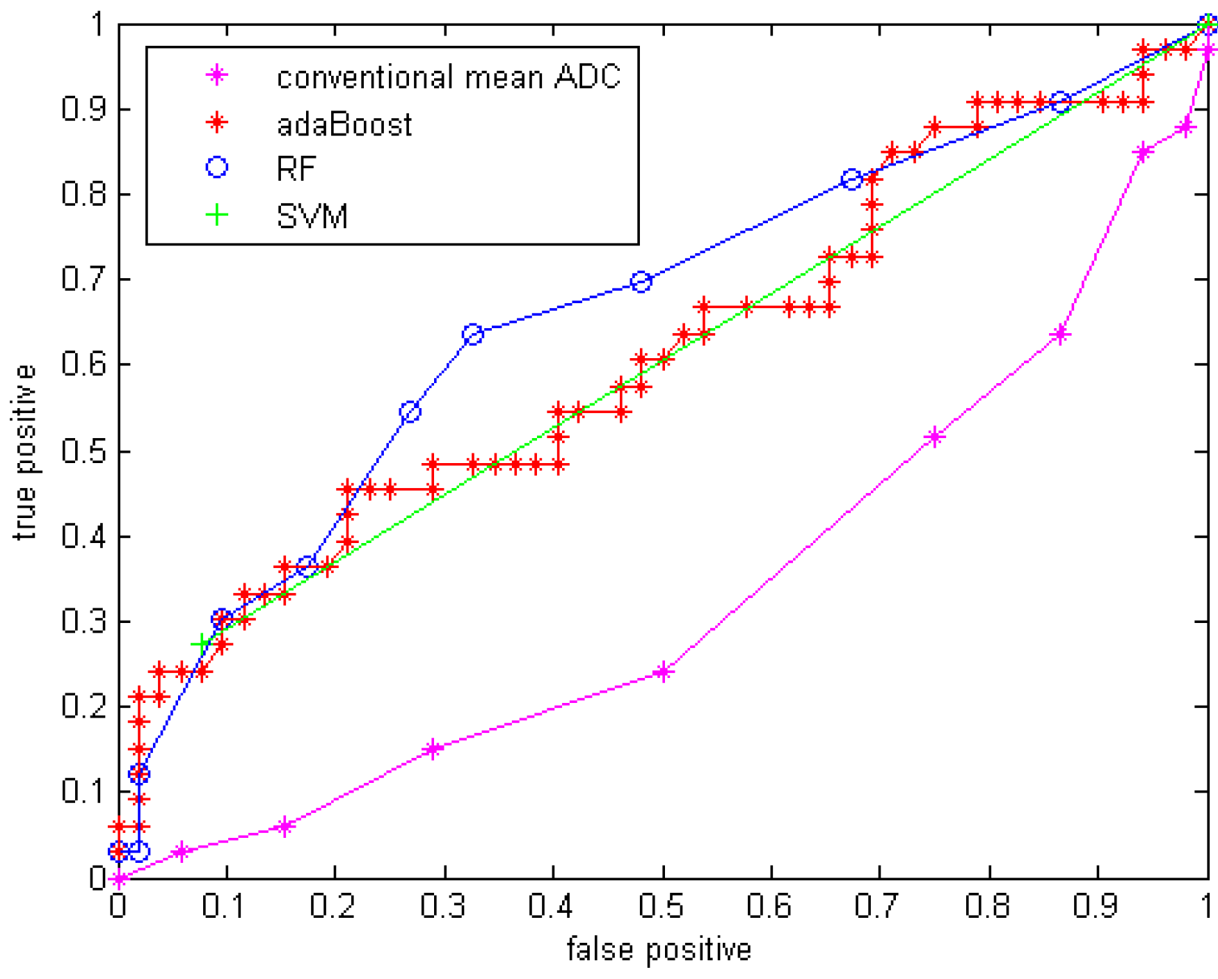
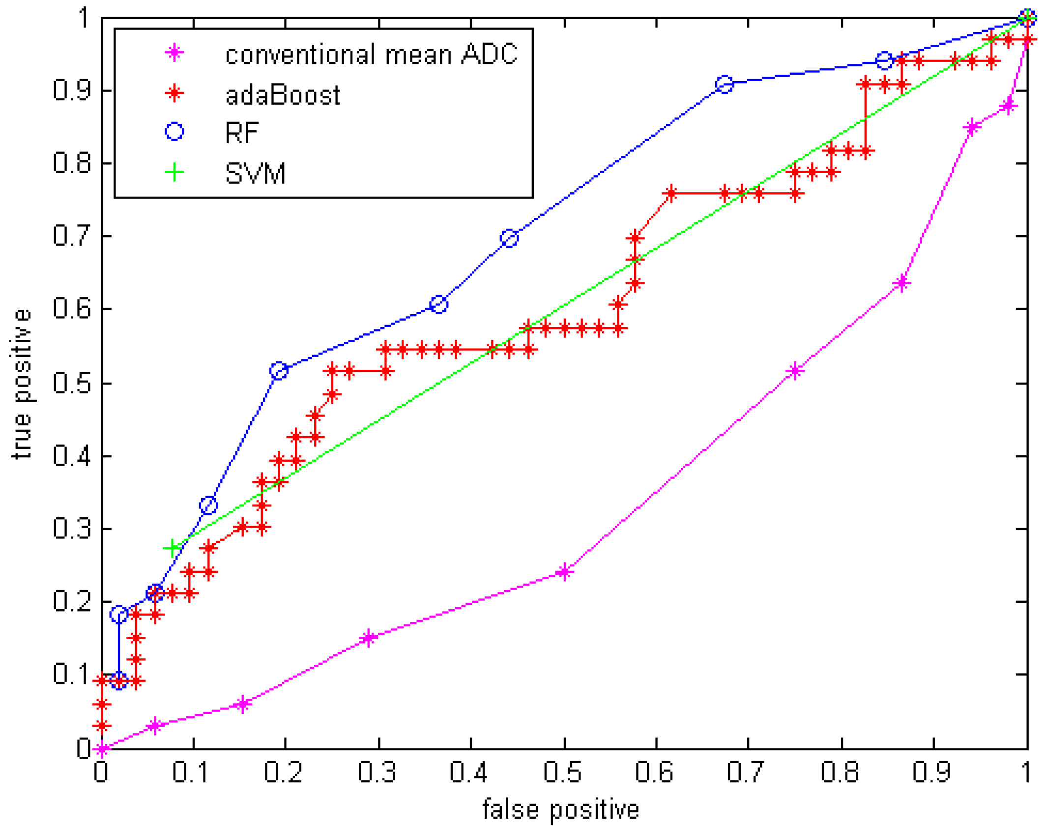
Compared to using only the mean ADC value, the quantitative statistical histogram features and the proposed classification system tremendously improved the accuracy from 29.4% to 69.41% (Az increased from 0.33 to 0.70). The statistical analysis indicates that all three classifiers are significantly different from the conventional mean ADC method with our dataset. Compared to general statistical histogram features, the classification with GMM features using random forest technique slightly improved the accuracy from 65.88% to 69.41%, while adaBoost and RF classifiers generated the same accuracy no matter whether GMM features were included. There is no significant difference between the three machine-learned classifiers.

The conventional mean ADC method performs worse than a random classifier (Az < 0.5). The reason is that conventionally researchers hypothesized that mean ADC increases because the tumor cell density decrease after an effective treatment. This assumption may not be valid for our dataset, because it involves in an anti-angiogenesis drug, which suppresses the cancer cell growth without necessary killing tumor cells (decreasing their density) at an early stage (5-7 weeks). Another possible reason is that in our dataset many of the GBM tumors are recurrent GBM tumors that are usually necrotic. The treatment tends to reduce necrosis and edema, which will diminish ADC. Essentially there are two competing processes at work: cell density, edema and necrosis [25].

Another state-of-art study included features that capture spatial information in tumor heterogeneity features. Functional diffusion map (fDM) [22,23] is a popular technique studying the ADC value increase or decrease voxel-by-voxel. Moffat et al. applied fDM to 20 patients, classified patients into the three categories: PR, SD and PD, and reported 100% accuracy [22]. However, the threshold they used for classification was determined from a single dataset of 20 patients used for both training and testing, while in our experiments, a cross validation analysis was performed. In Moffat et al’s study, they explored the assessment of fractionated radiation therapy for different types of brain tumors with 20 patients scanned on the same scanner [22]. However, in our study, we focused on the GBM brain tumors treated by anti-angiogenesis drugs, which suppress the blood supply for the tumor cells and may not directly decrease the tumor cellularity. The difference in accuracy may come from the different mechanism of treatment. Additionally, our dataset is from GBM drug trials across multiple sites, thus our preliminary study is an important contribution for exploring DWI as an early imaging biomarker in a real pharmaceutical drug trial. In future work, we will extract texture feature to include spatial information, and shape features will be extracted as well. By introducing a new richer feature set indicating more useful tumor information, we aim to include more information about tumors and further improve the performance of the classification system.

One limitation of this study is that we classified CR, PR and SD as responders for the ground truth to achieve a binary classification. Since SD and PR may have different patterns in terms of their ADC histogram change, a multi-category classification system will be explored in future work. Another limitation of the study is that we used the Macdonald criteria at the eighth or tenth week after treatment for determining treatment response. In future work, time-to-progression and survival time will be a better endpoint to classify treatment response. Another limitation comes from the 3D ROI mapping tool. This tool is more computationally efficient compared to the co-registration techniques, but it cannot correct for patient motion. Therefore, in our study, a board-certified radiologist’s visually checked and edited all segmentation results as needed. In the future, a more sophisticated registration method with an image similarity measure may improve the accuracy of the tumor contours on ADC maps, and consequently improve the accuracy of the extracted features and the classifier performance.

ADC values obtained on pre-operative MRI scans are reported to be of prognostic value in patients with glioblastoma [25,42]. The term "prognosis" refers to predicting the likely outcome of treatment. ADC, reported to be inversely proportional to tumor cellularity, is gaining interest in predicting GBM tumor prognosis. Our proposed framework now uses changes in DW-MRI for early prediction of treatment response; however, the framework with feature extraction and machine learning technique could be generalized to pre-treatment DW-MRI for prognosis prediction.

In this study, we developed a CADrx framework with machine learning techniques to automatically predict tumor treatment response before the size change using DW-MRI. In our preliminary study, our major contributions are extracting statistical ADC histogram features, applying GMM to model the ADC histogram to interpret the competing effects of cellular density and edema, and applying machine learning techniques using all the extracted features. Cell density and edema may be reflected in ADC values before size changes are apparent on standard MRI sequences. Therefore, ADC holds promise as a biomarker, in determining both which tumors are more likely to respond to treatment and which tumors are actually responding.

In conclusion, this work shows that a CADrx system using quantitative ADC histogram features and a machine-learned classifier has better performance in treatment response assessment over conventional analysis using only a mean ADC value. This will have major implications for clinical trials. This work has potential clinical significance for early treatment response assessment in GBM.

References

1. Giger, M.L. Computer-aided diagnosis in medical imaging — A new era in image interpretation; Technical Report; World Markets Research Centre: London, UK, 2000; pp. 75–78. [Google Scholar]
2. Ross, B.D.; Moffat, B.A.; Lawrence, T.S.; Mukherji, S.K.; Gebarski, S.S.; Quint, D.J.; Johnson, T.D.; Junck, L.; Robertson, P.L.; Muraszko, K.M.; Dong, Q.; Meyer, C.R.; Bland, P.H.; McConville, P.; Geng, H.; Rehemtulla, A.; Chenevert, T.L. Evaluation of cancer therapy using diffusion magnetic resonance imaging. Mol. Cancer Ther. 2003, 2, 581–587. [Google Scholar] [PubMed]
3. Padhani, A.R.; Liu, G.; Mu-Koh, D.; Chenevert, T.L.; Thoeny, H.C.; Takahara, T.; Dzik-Jurasz, A.; Ross, B.D.; Cauteren, M.V.; Collins, D.; Hammoud, D.A.; Rustin, G.J.S.; Taouli, B.; Choyke, P.L. Diffusion-weighted magnetic imaging as a cancer biomarker: consensus and recommendations. Neoplasia 2009, 11, 102–125. [Google Scholar] [CrossRef] [PubMed]
4. Phillips, W.E.; Velthuizen, R.P.; Phupanich, S.; Hall, L.O.; Clarke, L.P.; Silbiger, M.L. Applications of fuzzy C-means segmentation technique for tissue differentiation in MR images of a hemorrhagic glioblastoma multiforme. J. Magn. Reson. Imaging 1995, 13, 277–290. [Google Scholar] [CrossRef]
5. Clark, M.C.; Hall, L.O.; Goldgof, D.B.; Velthuizen, R.; Murtagh, R.; Silbiger, M.S. Automatic tumor segmentation using knowledge-based techniques. IEEE Trans. Med. Imaging 1998, 17, 187–201. [Google Scholar] [CrossRef] [PubMed]
6. Fletcher-Heath, L.M.; Hall, L.O.; Goldgof, D.B.; Murtagh, R.F. Automatic segmentation of non-enhancing brain tumors in magnetic resonance images. Artif. Intell. Med. 2001, 21, 43–63. [Google Scholar] [CrossRef]
7. Prastawa, M.; Bullitt, E.; Moon, N.; Leemput, K.V.; Gerig, G. Automatic brain tumor segmentation by subject specific modification of atlas priors. Acad. Radiol. 2003, 10, 1341–1348. [Google Scholar] [CrossRef]
8. Kaus, M.; Warfield, S.; Nabavi, A.; Black, P.M.; Jolesz, F.A.; Kikinis, R. Automated segmentation of mr images of brain tumors. Radiology 2001, 218, 586–591. [Google Scholar] [CrossRef] [PubMed]
9. Ho, S.; Bullitt, E.; Gerig, G. Level set evolution with region competition: Automatic 3-d segmentation of brain tumors. In Proceedings of International Conference on Pattern Recognition, Quebec, Canada, August, 2002; pp. 532–535.
10. Vinitski, S.; Gonzalez, C.F.; Knobler, R.; Andrews, D.; Iwanaga, T.; Curtis, M. Fast tissue segmentation based on a 4D feature map in characterization of intracranial lesions fast tissue segmentation based on a 4D feature map in characterization of intracranial lesions. J. Magn. Reson. Imaging 1999, 9, 768–776. [Google Scholar] [CrossRef]
11. Lee, C.H.; Schmidt, M.; Murtha, A.; Bistritz, A.; Sander, J.; Greiner, R. Segmenting brain tumor with conditional random fields and support vector machines. In Proceedings of Workshop on Computer Vision for Biomedical Image Applications at International Conference on Computer Vision, Beijing, China, October, 2005; Vol. 3765, pp. 469–478.
12. Zhu, Y.; Yan, H. Computerized tumor boundary detection using a hopfield neural network. LEEE Trans. Med. Imaging 1997, 16, 55–67. [Google Scholar]
13. Zhang, J.; Ma, K.; Er, M.H.; Chong, V. Tumor segmentation from magnetic resonance imaging by learning via one-class support vector machine. In Proceedings of International Workshop on Advanced Image Technology, Singapore, January, 2004; pp. 207–211.
14. Niea, J.; Xue; Liu, T.; Young, G.S.; Setayesh, K.; Guo, L.; Wong, S.T.C. Automated brain tumor segmentation using spatial accuracy-weighted hidden Markov Random Field. Comput. Med. Imaging Graph. 2009, 33, 431–441. [Google Scholar] [CrossRef] [PubMed]
15. Corso, J.J.; Sharon, E.; Dube, S.; El-Saden, S.; Sinha, U.; Yuille, A. Efficient Multilevel Brain Tumor Segmentation with Integrated Bayesian Model Classification. IEEE Trans. Med. Imaging 2008, 27, 629–640. [Google Scholar] [CrossRef] [PubMed]
16. Liu, J.; Udupa, J.; Odhner, D.; Hackney, D.; Moonis, G. A system for brain tumor volume estimation via mr imaging and fuzzy connectedness. Comput. Med. Imaging Graph. 2005, 29, 21–34. [Google Scholar] [CrossRef] [PubMed]
17. Dube, S.; Corso, J.J.; Yuille, A.; Cloughesy, T.F.; El-Saden, S.; Sinha, U. Hierarchical Segmentation of Malignant Gliomas via Integrated Contextual Filter Response. Proc. SPIE 2008, 6914, 69143Y. [Google Scholar]
18. Dube, S.; Corso, J.J.; Cloughesy, T.F.; El-Saden, S.; Yuille, A.; Sinha, U. Automated MR image processing and analysis of malignant brain tumors: enabling technology for data mining. In Data Mining Systems Analysis and Optimization in Biomedicine; American Institute of Physics Proceedings: New York, NY, USA, 2007; Vol. 953, pp. 64–84. [Google Scholar]
19. US Food and Drug Administration. Guidance for industry: clinical trial endpoints for the approval of cancer drugs and biologics. Federal Register 2007, 72, No. 94. [Google Scholar]
20. Chenevert, T.L.; Stegman, L.D.; Taylor, J.M.; Robertson, P.L.; Greenberg, H.S.; Rehemtulla, A.; Ross, B.D. Diffusion magnetic resonance imaging: an early surrogate marker of therapeutic efficacy in brain tumors. J. Natl. Cancer Inst. 2000, 92, 2029–2036. [Google Scholar] [CrossRef] [PubMed]
21. Mardor, Y.; Pfeffer, R.; Spiegelmann, R.; Roth, Y.; Maier, S.E.; Nissim, O.; Berger, R.; Glicksman, A.; Baram, J.; Orenstein, A.; Cohen, J.S.; Tichler, T. Early detection of response to radiation therapy in patients with brain malignancies using conventional and high b-value diffusion-weighted magnetic resonance imaging. J. Clin. Oncol. 2003, 21, 1094–1100. [Google Scholar] [CrossRef] [PubMed]
22. Moffat, B.A.; Chenevert, T.L.; Meyer, C.R.; Mckeever, P.E.; Hall, D.E.; Hoff, B.A.; Johnson, T.D.; Rehemtulla, A.; Ross, B.D. The functional diffusion map: a noninvasive MRI biomarker for early stratification of clinical brain tumor response. PANS 2005, 102, 5524–5529. [Google Scholar] [CrossRef] [PubMed]
23. Hamstra, D.A.; Chenevert, T.L.; Moffat, B.A.; Johnson, T.D.; Meyer, C.R.; Mukherji, S.K.; Quint, D.J.; Gebarski, S.S.; Fan, X.; Tsien, C.I.; Lawrence, T.S.; Junck, L.; Rehemtulla, A.; Ross, B.D. Evaluation of the functional diffusion map as an early biomarker of time-to-progression and overall survival in high-grade glioma. PNAS 2005, 102, 16759–16764. [Google Scholar] [CrossRef] [PubMed]
24. Huo, J.; Kim, H.J.; Pope, W.B.; Okada, K.; Alger, J.R.; Wang, Y.; Goldin, J.G.; Brown, W.S. Histogram-based classification with Gaussian mixture modeling for GBM tumor treatment response using ADC map. Proc. SPIE 2009, 7260, 72601Y. [Google Scholar]
25. Pope, W.B.; Kim, H.J.; Huo, J.; Alger, J.R.; Brown, W.S.; Gjertson, D.; Sai, V.; Young, J.R.; Tekchandani, L.; Cloughesy, T.; Mischel, P.S.; Lai, A.; Nghiemphu, P.; Rahmanuddin, S.; Goldin, J.G. Recurrent glioblastoma multiforme: ADC histogram analysis predicts response to bevacizumab treatment. Radiology 2009, 252, 1–8. [Google Scholar] [CrossRef] [PubMed]
26. Sajda, P. Machine learning for detection and diagnosis of disease. Annu. Rev. Biomed. Eng. 2006, 8, 537–65. [Google Scholar] [CrossRef] [PubMed]
27. Freund, Y.; Schapire, R.E. A short introduction to boosting. J. Jpn. Soc. For. Artif. Intell. 1999, 14, 771–780. [Google Scholar]
28. Duda, R.O.; Hart, P.E.; Stork, D.H. Pattern classification; Wiley Interscience: Malden, MA, USA, 2000. [Google Scholar]
29. Ho, T.K. Random decision forest. In Proceedings of the 3rd International Conference on Document Analysis and Recognition, Montreal, Canada, August, 1995; pp. 278–282.
30. Breiman, L. Random decision forest. Mach. Learn. 2001, 45, 5–32. [Google Scholar] [CrossRef]
31. Vapnik, V. Estimation of Dependencies Based on Empirical Data; Nauka: Moscow, Russia, 1979. [Google Scholar]
32. Bishop, C. Neural Networks for Pattern Recognition; Clarendon Press: Oxford, UK, 1995. [Google Scholar]
33. http://en.wikipedia.org/wiki/Support_vector_machine (accessed November 10, 2009).
34. Burbidge, R.; Trotter, M.; Buxton, B.; Holden, S. Drug design by machine learning: support vector machines for pharmaceutical data analysis. Comput. And. Chem 2001, 26, 5–14. [Google Scholar] [CrossRef]
35. Huo, J.; Alger, J.R.; Kim, H.J.; Pope, W.B.; Okada, K.; Goldin, J.G.; Brown, M.S. Between-scanner variation in normal white matter ADC in the setting of a multi-center clinical trial. Ismrm 2009, (in press). [Google Scholar]
36. Otsu , N. A threshold selection method from gray level histograms. IEEE Trans. Syst. Man. Cybern. 1979, 9, 62–66. [Google Scholar]
37. Adams, R.; Bischof, L. Seeded region growing. IEEE Trans. Syst. Man. Cybern. Int. 1994, 16, 641–647. [Google Scholar] [CrossRef]
38. Rubner, Y.; Tomasi, C.; Guibas, L.J. A metric for distributions with applications to image databases. In Proceedings of ICCV, Bombay, India, January, 1998; pp. 59–66.
39. Ling, H.; Okada, K. An efficient Earth mover's distance algorithm for robust histogram comparison. IEEE Trans. Patt. Anal. Mach. Intell. 2007, 29, 840–853. [Google Scholar] [CrossRef] [PubMed]
40. Witten, I.H.; Frank, E. Data Mining: Practical Machine Learning Tools and Techniques; Morgan Kaufmann: San Francisco, CA, USA, 2005. [Google Scholar]
41. Yamasaki, F.; Sugiyama, K.; Ohtaki, M.; Takeshima, Y.; Abed, N.; Akiyamad, Y.; Takabad, J.; Amatyac, V.J.; Saitoa, T.; Kajiwaraa, Y.; Hanayaa, R.; Kurisua, K. Glioblastoma treated with postoperative radio-chemotherapy: Prognostic value of apparent diffusion coefficient at MR imaging. Eur.J. Aiol. 2009, (in press). [Google Scholar] [CrossRef] [PubMed]
42. Marzban, C. The ROC curve and the area under it as a performance measure. Weather Forecast. 2004, 19, 1106–1114. [Google Scholar] [CrossRef]
43. Huhn, S.L.; Mohapatra, G.; Bollen, A.; Lamborn, K.; Prados, M.D.; Feuerstein, B.G. Chromosomal abnormalities in glioblastoma multiforme by comparative genomic hybridization: correlation with radiation treatment outcome. Clin. Cancer Res. 1999, 5, 1435–1443. [Google Scholar] [PubMed]