1. Introduction
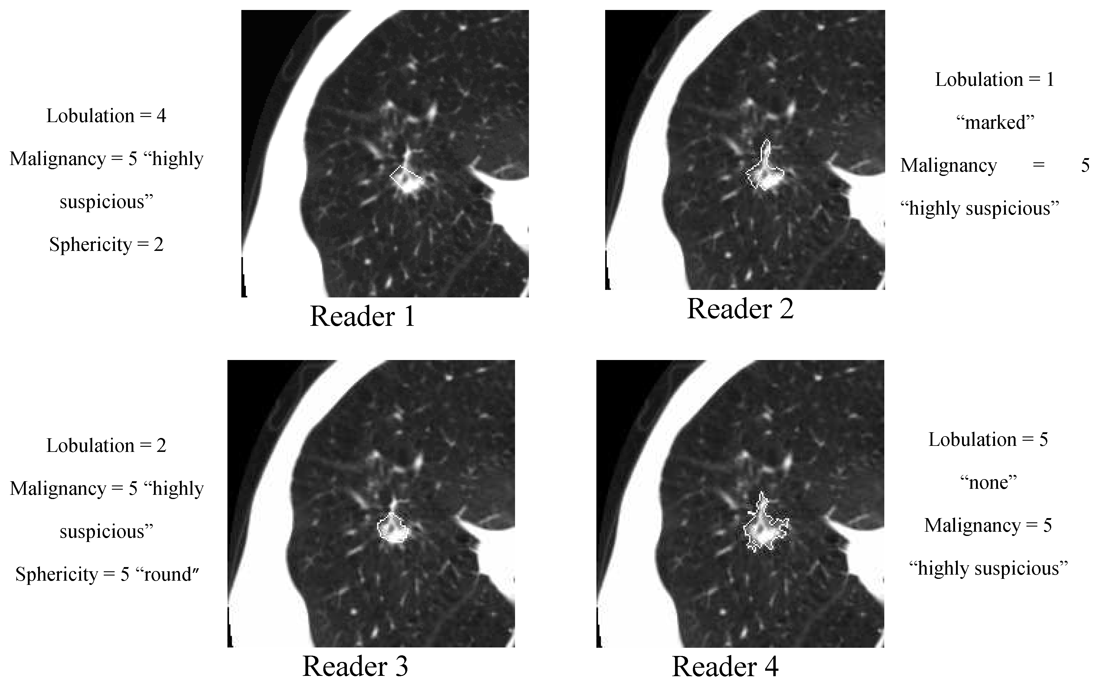
Interpretation performance varies greatly among radiologists when assessing lung nodules on computed tomography (CT) scans. A good example of such variability is the Lung Image Database Consortium (LIDC) dataset [
1] for which out of 914 distinct nodules identified, delineated, and semantically characterized by up to four different radiologists, there are only 180 nodules on average across seven semantic characteristics on which at least three radiologists agreed with respect to the semantic label (characteristic rating) applied to the nodule. Computer-aided diagnosis (CADx) systems can act as a second reader by assisting radiologists in interpreting nodule characteristics in order to improve their efficiency and accuracy.
In our previous work [
2] we developed a semi-automatic active-learning approach [
3] for predicting seven lung nodule semantic characteristics: spiculation, lobulation, texture, sphericity, margin, subtlety, and malignancy. The approach was intended to handle the large variability among interpretations of the same nodule by different radiologists. Using nodules with a high level of agreement as initial training data, the algorithm automatically labeled and added to the training data those nodules which had inconsistency in their interpretations. The evaluation of the algorithm was performed on the LIDC dataset publicly available at the time of publication, specifically on 149 distinct nodules present in the CT scans of 60 patients.
A new LIDC dataset consisting of 914 distinct nodules from 207 patients was made publicly available as of June 2009. This has opened the way to further investigate the robustness of our proposed approach. Given the highly non-normal nature of medical data in general and of the LIDC dataset in particular (for example, on the set of 236 nodules for which at least three radiologists agree with respect to the spiculation characteristic, 231 of these nodules are rated with a 1 (”marked spiculation”) and only five nodules are rated with ratings from 2 to 5 (where 5 “no spiculation”), we include in our research design a new study to evaluate the effects of balanced and unbalanced datasets on the proposed ensemble’s performance for each of the seven characteristics. Furthermore, we investigate the agreement between our proposed computer-aided diagnostic characterization (CADc) approach and the LIDC radiologists’ semantic characterizations using the weighted kappa statistic [
4] which takes into account the general magnitude of the radiologists’ agreement and weighs the differences in their disagreements with respect to every available instance. Finally, we include a new research study to investigate the effects of the variation/disagreement present in the manual lung nodule delineation/segmentation on performance of the ensemble of classifiers.
The rest of the paper is organized as follows: we present a literature review relevant to our work in
Section 2, the National Cancer Institute (NCI) LIDC dataset and methodology in
Section 3, the results in
Section 4, and our conclusions and future work in
Section 5.
2. Related Work
A number of CAD systems have been developed in recent years for automatic classification of lung nodules. McNitt-Gray
et al. [
5,
6] used nodule size, shape and co-occurrence texture features as nodule characteristics to design a linear discriminant analysis (LDA) classification system for malignant versus benign nodules. Lo
et al. [
7] used direction of vascularity, shape, and internal structure to build an artificial neural network (ANN) classification system for the prediction of the malignancy of nodules. Armato
et al. [
8] used nodule appearance and shape to build an LDA classification system to classify pulmonary nodules into malignant versus benign classes. Takashima
et al. [
9,
10] used shape information to characterize malignant versus benign lesions in the lung. Shah
et al. [
11] compared the malignant
vs. benign classification performance of OneR [
12] and logistic regression classifiers learned on 19 attenuation, size, and shape image features; Samuel
et al. [
13] developed a system for lung nodule diagnosis using Fuzzy Logic. Furthermore, Sluimer
et al. [
14] and more recently Goldin
et al. [
15] summarized in their survey papers the existing lung nodule segmentation and classification techniques.
There are also research studies that use clinical information in addition to image features to classify lung nodules. Gurney
et al. [
16,
17] designed a Bayesian classification system based on clinical information, such as age, gender, smoking status of the patient,
etc., in addition to radiological information. Matsuki
et al. [
18] also used both clinical information and sixteen features scored by radiologists to design an ANN for malignant versus benign classification. Aoyama
et al. [
19] used two clinical features in addition to forty-one image features to determine the likelihood measure of malignancy for pulmonary nodules on low-dose CT images.
Although the work cited above provides convincing evidence that a combination of image features can indirectly encode radiologists’ knowledge about indicators of malignancy (Sluimer
et al. [
14]), the precise mechanism by which this correspondence happens is unknown. To understand this mechanism, there is a need to explore several approaches for finding the relationships between the image features and radiologists’ annotations. Kahn
et al. [
20] emphasized recently the importance of this type of research; the knowledge gathered from the post-processed images and its incorporation into the diagnosis process could simplify and accelerate the radiology interpretation process.
Notable work in this direction is the work by Barb
et al. [
21] and Ebadollahi
et al. [
22,
23]. Barb
et al. proposed a framework that uses semantic methods to describe visual abnormalities and exchange knowledge in the medical domain. Ebadollahi
et al. proposed a system to link the visual elements of the content of an echocardiogram (including the spatial-temporal structure) to external information such as text snippets extracted from diagnostic reports. Recently, Ebadollahi
et al. demonstrated the effectiveness of using a semantic concept space in multimodal medical image retrieval.
In the CAD domain, there is some preliminary work to link images to BI-RADS. Nie
et al. [
24] reported results linking the gray-level co-occurrence matrix (GLCM) entropy and GLCM sum average to internal enhancement patterns (homogenous versus heterogeneous) defined in BI-RADS, while Liney
et al. [
25] linked complexity and convexity image features to the concept of margin and circularity to the concept of shape. Our own work [
26,
27] can also be considered one of the initial steps in the direction of mapping lung nodule image features first to perceptual categories encoding the radiologists’ knowledge about lung interpretation and further to the RadLex lexicon [
28].
In this paper we propose a semi-supervised probabilistic learning approach to deal with both the inter-observer variability and the small set of labeled data (annotated lung nodules). Given the ultimate use of our proposed approach as a second reader in the radiology interpretation process, we investigate the agreement between the ensemble of classifiers and the LIDC panel of experts as well as the performance accuracy of the ensemble of classifiers. The accuracy of the ensemble is calculated as the number of correctly classified instances over the total number of instances. The agreement is measured using weighted kappa statistic as introduced by Cohen [
4,
29]. The weighted kappa statistic takes into account the level of disagreement and the specific category on which raters agreed for each observed case, reflecting the importance of a certain rating. Originally, the kappa statistic was intended to measure the agreement between two raters across a number of cases, where the pair of raters is fixed for all cases. Fleiss [
30] proposed a generalization of kappa statistics which measures the overall agreement across multiple observations when more than two raters were interpreting a specific case. Landis and Koch [
31] explored the use of kappa statistics for assessing the majority agreement by modifying the unified agreement evaluation approach that they proposed in a previously published paper [
32]. An approach proposed by Kraemer [
33] extended the technique proposed by Fleiss [
34] to situations in which there are a multiple number of observations per subject and a multiple, inconstant number of possible responses per observation. More recently, Viera and Garrett [
35] published a paper that describes and justifies a possible interpretation scale for the value of kappa statistics obtained in the evaluation of inter-observer agreement. They propose to split the range of possible values of the kappa statistic into several intervals and assign an ordinal value to each of them as shown in
Table 1. We will use this interpretation scale to quantify the agreement between the panel of LIDC experts and the ensemble of classifiers.
Table 1.
Kappa statistics interpretation scale.
Table 1.
Kappa statistics interpretation scale.
| k-value (%) | Strength of Agreement beyond Chance |
|---|
| <0 | Poor |
| 0–0.2 | Slight |
| 0.21–0.4 | Fair |
| 0.41–0.6 | Moderate |
| 0.61–0.8 | Substantial |
| 0.81–1 | Almost perfect |
3. Methodology
3.1. LIDC dataset
The publicly available LIDC database (downloadable through the National Cancer Institute’s Imaging Archive web site-
http://ncia.nci.nih.gov/) provides the image data, the radiologists’ nodule outlines, and the radiologists’ subjective ratings of nodule characteristics for this study. The LIDC database currently contains complete thoracic CT scans for 208 patients acquired over different periods of time and with various scanner models resulting in a wide range of values of the imaging acquisition parameters. For example, slice thickness ranges between 0.6 mm and 4.0 mm, reconstruction diameter ranges between 260 mm and 438 mm, exposure ranges between 3 ms and 6,329 ms, and the reconstruction kernel has one of the following values: B, B30f, B30s, B31f, B31s, B45f, BONE, C, D, FC01, or STANDARD.
Table 2.
LIDC nodule characteristics with corresponding rating scale.
Table 2.
LIDC nodule characteristics with corresponding rating scale.
| Characteristic | Notes and References | Possible Scores |
|---|
| Calcification | Pattern of calcification present in the nodule | 1. Popcorn
2. Laminated
3. Solid
4. Non-central
5. Central
6. Absent |
| Internal structure | Expected internal composition of the nodule | 1. Soft Tissue
2. Fluid
3. Fat
4. Air |
| Lobulation | Whether a lobular shape is apparent from the margin or not | 1. Marked
2. .
3. .
4. .
5. None |
| Malignancy | Likelihood of malignancy of the nodule - Malignancy is associated with large nodule size while small nodules are more likely to be benign. Most malignant nodules are non-calcified and have spiculated margins. | 1. Highly Unlikely
2.Moderately Unlikely
3. Indeterminate
4.Moderately Suspicious
5. Highly Suspicious |
| Margin | How well defined the margins of the nodule are | 1. Poorly Defined
2. .
3. .
4. .
5. Sharp |
| Sphericity | Dimensional shape of nodule in terms of its roundness | 1. Linear
2. .
3. Ovoid
4. .
5. Round |
| Spiculation | Degree to which the nodule exhibits spicules, spike-like structures, along its border - Spiculated margin is an indication of malignancy | 1. Marked
2. .
3. .
4. .
5. None |
| Subtlety | Difficulty in detection - Subtlety refers to the contrast between the lung nodule and its surrounding | 1. Extremely Subtle
2. Moderately Subtle
3. Fairly Subtle
4.Moderately Obvious
5. Obvious |
| Texture | Internal density of the nodule - Texture plays an important role when attempting to segment a nodule, since part-solid and non-solid texture can increase the difficulty of defining the nodule boundary | 1. Non-Solid
2. .
3. Part Solid/(Mixed)
4. .
5. Solid |
The XML files accompanying the LIDC DICOM images contain the spatial locations of three types of lesions (nodules < 3 mm in maximum diameter, but only if not clearly benign; nodules > 3 mm but <30 mm regardless of presumed histology; and non-nodules > 3 mm) as marked by a panel of up to 4 LIDC radiologists. For any lesion marked as a nodule > 3 mm, the XML file contains the coordinates of nodule outlines constructed by any of the 4 LIDC radiologists who identified that structure as a nodule > 3 mm. Moreover, any LIDC radiologist who identified a structure as a nodule > 3 mm also provided subjective ratings for 9 nodule characteristics (
Table 2): subtlety, internal structure, calcification, sphericity, margin, lobulation, spiculation, texture, and malignancy likelihood. For example, the texture characteristic provides meaningful information regarding nodule appearance (“Non-Solid”, “Part Solid/(Mixed)”, “Solid”) while malignancy characteristic captures the likelihood of malignancy (“Highly Unlikely”, “Moderately Unlikely”, “Indeterminate”, “Moderately Suspicious”, “Highly Suspicious”) as perceived by the LIDC radiologists. The process by which the LIDC radiologists reviewed CT scans, identified lesions, and provided outlines and characteristic ratings for nodules > 3 mm has been described in detail by McNitt-Gray
et al. [
36].
The nodule outlines and the seven of the nodule characteristics were used extensively throughout this study. Note that the LIDC did not impose a forced consensus; rather, all of the lesions indicated by the radiologists at the conclusion of the unblinded reading sessions were recorded and are available to users of the database. Accordingly, each lesion in the database considered to be a nodule > 3 mm could have been marked as such by only a single radiologist, by two radiologists, by three radiologists, or by all four LIDC radiologists. For any given nodule, the number of distinct outlines and the number of sets of nodule characteristic ratings provided in the XML files would then be equal to the number of radiologists who identified the nodule.
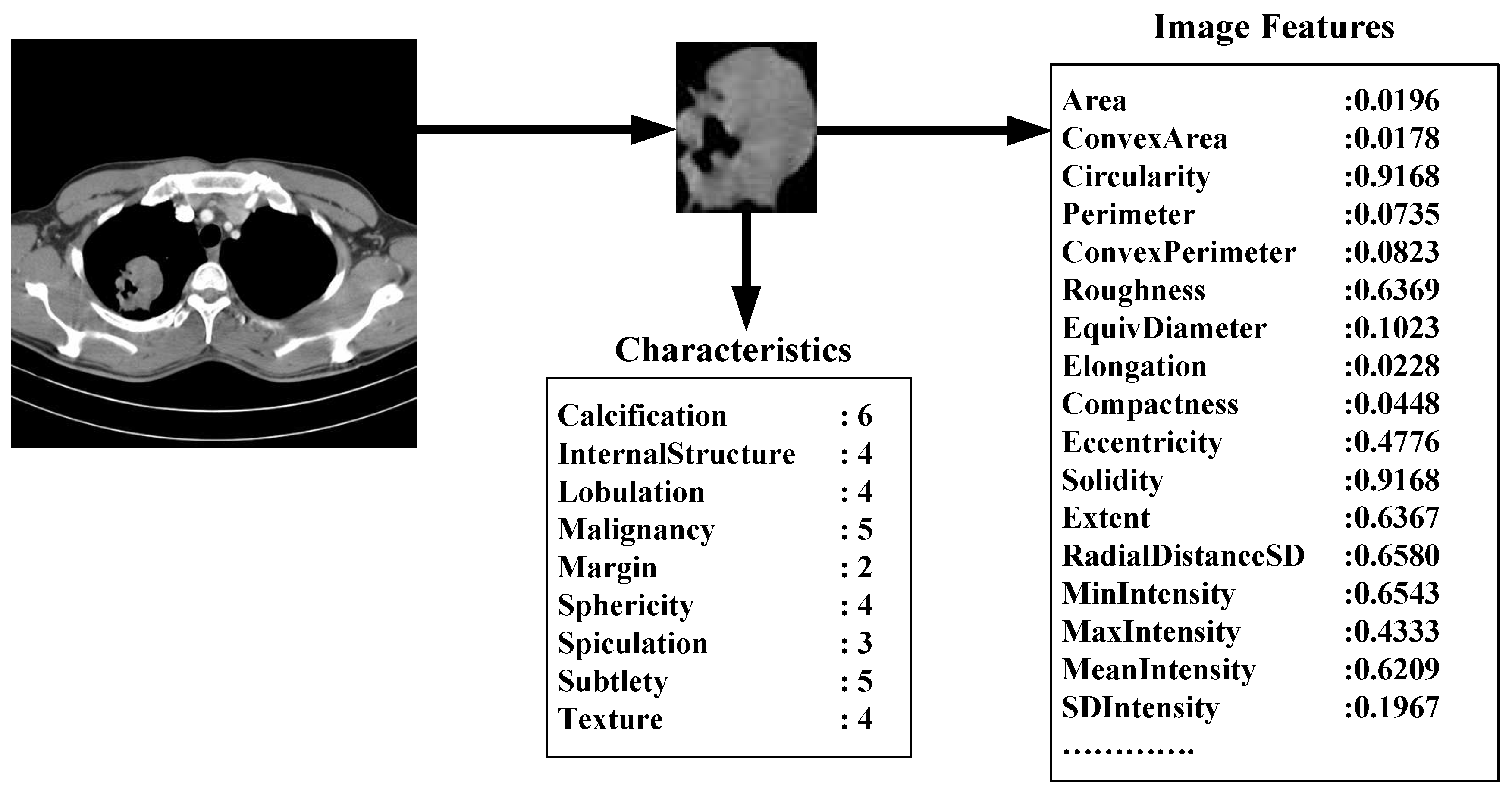
Size Features
We use the following seven features to quantify the size of the nodules: area, ConvexArea, perimeter, ConvexPerimeter, EquivDiameter, MajorAxisLength, and MinorAxisLength. The area and perimeter image features measure the actual number of pixels in the region and on the boundary, respectively. The ConvexArea and ConvexPerimeter measure the number of pixels in the convex hull and on the boundary of the convex hull corresponding to the nodule region. EquivDiameter is the diameter of a circle with the same area as the region. Lastly, the MajorAxisLength and MinorAxisLength give the length (in pixels) of the major and minor axes of the ellipse that has the same normalized second central moments as the region.
Shape Features
We use eight common image shape features: circularity, roughness, elongation, compactness, eccentricity, solidity, extent, and the standard deviation of the radial distance. Circularity is measured by dividing the circumference of the equivalent area circle by the actual perimeter of the nodule. Roughness can be measured by dividing the perimeter of the region by the convex perimeter. A smooth convex object, such as a perfect circle, will have a roughness of 1.0. The eccentricity is obtained using the ellipse that has the same second-moments as the region. The eccentricity is the ratio of the distance between the foci of the ellipse and its major axis length. The value is between 0 (a perfect circle) and 1 (a line). Solidity is the proportion of the pixels in the convex hull of the region to the pixels in the intersection of the convex hull and the region. Extent is the proportion of the pixels in the bounding box (the smallest rectangle containing the region) that are also in the region. Finally, the RadialDistanceSD is the standard deviation of the distances from every boundary pixel to the centroid of the region.
Intensity Features
Gray-level intensity features used in this study are simply the minimum, maximum, mean, and standard deviation of the gray-level intensity of every pixel in each segmented nodule and the same four values for every background pixel in the bounding box containing each segmented nodule. Another feature, IntensityDifference, is the absolute value of the difference between the mean of the gray-level intensity of the segmented nodule and the mean of the gray-level intensity of its background.
Texture Features
Normally texture analysis can be grouped into four categories: model-based, statistical-based, structural-based, and transform-based methods. Structural approaches seek to understand the hierarchal structure of the image, while statistical methods describe the image using pure numerical analysis of pixel intensity values. Transform approaches generally perform some kind of modification to the image, obtaining a new “response” image that is then analyzed as a representative proxy for the original image. Model-based methods are based on the concept of predicting pixel values based on a mathematical model. In this research we focus on three well-known texture analysis techniques: co-occurrence matrices (a statistical-based method), Gabor filters (a transform-based method), and Markov Random Fields (a model based method).
Co-occurrence matrices focus on the distributions and relationships of the gray-level intensity of pixels in the image. They are calculated along four directions (0°, 45°, 90°, and 135°) and five distances (1, 2, 3, 4 and 5 pixels) producing 20 co-occurrence matrices. Once the co-occurrence matrices are calculated, eleven Haralick texture descriptors are then calculated from each co-occurrence matrix. Although each Haralick texture descriptor is calculated from each co-occurrence matrix, we averaged the features across all distance/direction pairs resulting in 11 (instead of 11 × 4 × 5) Haralick features per image.
Gabor filtering is a transform based method which extracts texture information from an image in the form of a response image. A Gabor filter is a sinusoid function modulated by a Gaussian and discretized over orientation and frequency. We convolve the image with 12 Gabor filters: four orientations (0°, 45°, 90°, and 135°) and three frequencies (0.3, 0.4, and 0.5), where frequency is the inverse of wavelength. We then calculate means and standard deviations from the 12 response images resulting in 24 Gabor features per image.
Markov Random Fields (MRFs) is a model based method which captures the local contextual information of an image. We calculate five features corresponding to four orientations (0°, 45°, 90°, 135°) along with the variance. We calculate feature vectors for each pixel by using a 9 estimation window. The mean of four different response images and the variance response image are used as our five MRF features.
3.3. Active DECORATE for lung nodule interpretation
We propose to find mappings based on a small labeled initial dataset that, instead of predicting a certain rating (class) for a semantic characteristic, will generate probabilities for all possible ratings of that characteristic. Our proposed approach is based on the DECORATE [
38] algorithm, which iteratively constructs an ensemble of classifiers by adding a small amount of data, artificially generated and labeled by the algorithm, to the data set and learning a new classifier on the modified data. The newly created classifier is kept in the ensemble if it does not decrease the ensemble’s classification accuracy. Active-DECORATE [
39] is an extension of the DECORATE algorithm that detects examples from the unlabeled pool of data that create the most disagreement in the constructed ensemble and adds them to the data after manual labeling. The procedure is repeated until a desired size of the data set or a predetermined number of iterations is reached. The difference between Active-DECORATE and our approach lies in the way examples from the unlabeled data are labeled at each repetition. While in Active-DECORATE, labeling is done manually by the user, our approach labels examples automatically by assigning them the labels (characteristics ratings, in the context of this research) with the highest probabilities/confidence as predicted by the current ensemble of classifiers.
Since the process of generating the ensemble of classifiers for every semantic characteristic is the same, we will explain below the general steps of our approach regardless of the semantic characteristic to be predicted. The only difference will consist of the initial labeled data that will be used for creation of the ensemble of classifiers. For each characteristic, the ensemble will be built starting with the nodules on which at least three radiologists’ agree with respect to that semantic characteristic (regardless of the other characteristics).
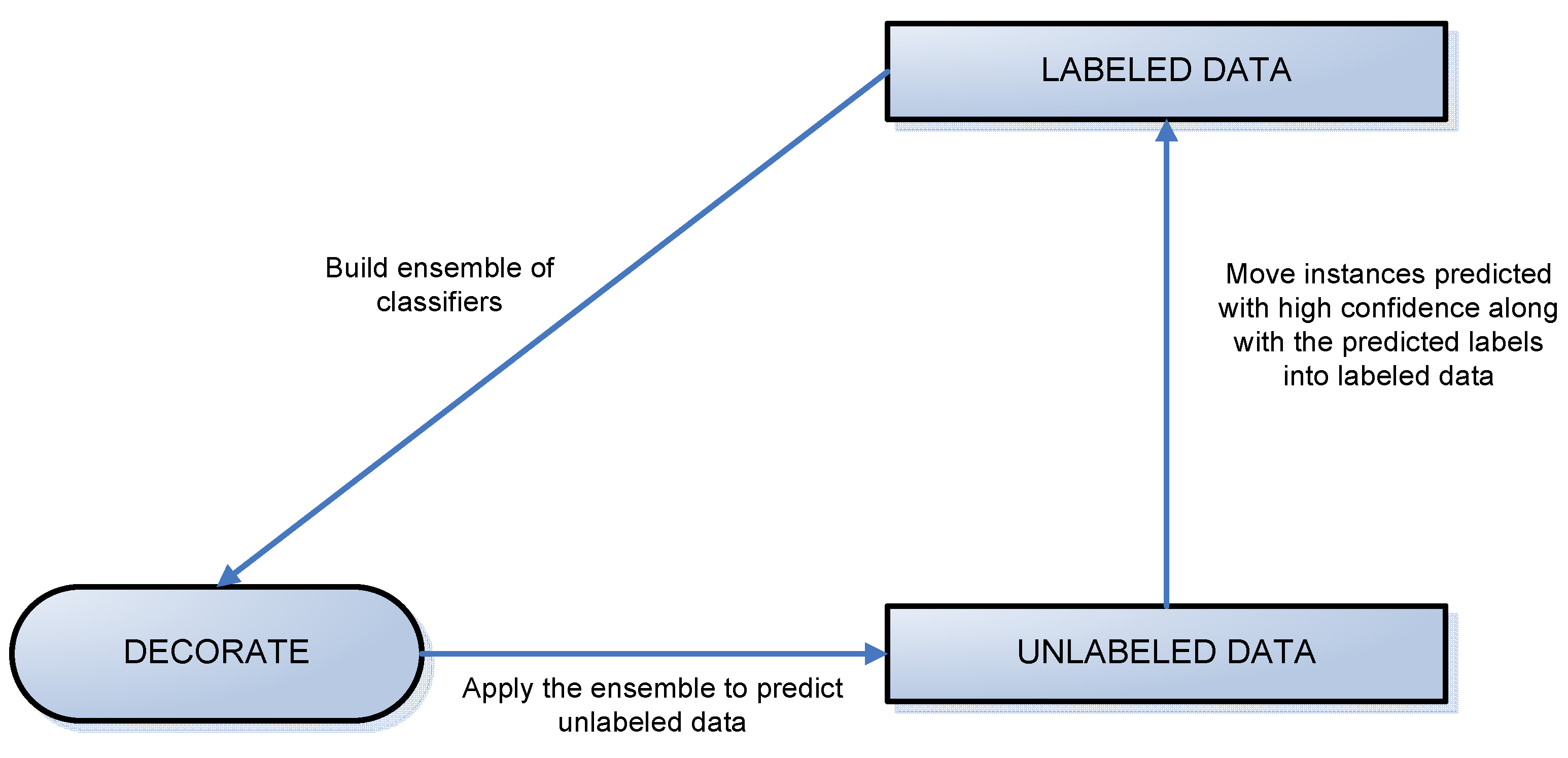
Figure 3.
A diagram of the labeling process.
Figure 3.
A diagram of the labeling process.
We divided the LIDC data into two datasets: labeled and unlabeled data, where labeled data included all instances of the nodules on which at least three radiologists agreed and unlabeled data contained all other instances (
Figure 3). The algorithms woks iteratively to move all examples from the unlabeled data set to the labeled data set. At each iteration, some instances were chosen for this transition using the results of classification specific to that iteration.
Instances were added to the labeled data set based on the confidence with which they were predicted. Instances predicted with probability higher than a threshold were added into the training set along with their predicted labels (ratings produced by CAD). When an iteration of the algorithm failed to produce any labels of sufficient confidence, every instance left in the unlabeled pool was added to the labeled data along with its original label (rating assigned by the radiologist). This is shown by the vertical arrow in
Figure 3. At this point, the ensemble of classifiers generated in the most recent iteration is the ensemble used to generate final classification and accuracy results.
The creation of the ensemble of classifiers at each iteration is driven by the DECORATE algorithm. The steps of the DECORATE algorithm are as follows: first, the ensemble is initialized by learning a classifier on the given labeled data. On subsequent steps, an additional classifier is learned by generating artificial training data and adding it to the existing training data. Artificial data is generated by randomly picking data points from a Gaussian approximation of the current labeled data set and labeling these data points in such a way that labels chosen differ maximally from the current ensemble’s predictions. After a new classifier is learned based on the addition of artificial data, the artificial data is removed from the labeled data set and the ensemble checked against the remaining (original, non-artificial) data. The decision on whether a newly created classifier should be kept in the ensemble depends on how this classifier affects the ensemble error. If the error increases, the classifier is discarded. The process is repeated until the ensemble reaches the desired size (number of classifiers) or a maximum number of iterations are performed. A visual representation of the algorithm’s steps is shown on
Figure 4.
To label a new unlabeled example x, each classifier Ci, in the ensemble C* provides probabilities for the class membership of x. We compute the class membership probabilities for the entire ensemble as:
where Y is the set of all possible classes (labels), and
![Algorithms 02 01473 i001]()
is the probability of example x belonging to class y
k according to the classifier C
i. The probability given by Equation 1 is used to identify the nodules predicted with high confidence.
In ensemble learning the ensemble can be composed out of classifiers of any type, such as artificial neural networks, support vector machines, decision trees, etc. In this paper, we are using decision trees (C4.5 implemented in WEKA [
40]) and the information gain criterion (Equation 2) for forming the trees [
41]:
where v is a value of attribute A, |S
v| is the subset of instances of S where A takes the value v, and |S| is the number of instances, and
where p
i is the proportion of instances in the dataset that has the target attribute i from C categories.
Figure 4.
The diagram of the DECORATE algorithm.
Figure 4.
The diagram of the DECORATE algorithm.
3.4. Evaluation of the CADc
In addition to the evaluation of the CADc performance with respect to its accuracy (the ratio of the correctly classified instances over the total number of instances), we investigate the effects of the variation in the manually delineated nodule boundaries across radiologists on the accuracy of the ensemble of classifiers. Furthermore, we evaluate the agreement between the ensemble’s predictions and the radiologists’ ratings using kappa statistics as presented below.
3.4.1. Variability index as a measure of variability in the lung nodule manual segmentation
We also investigated the accuracy of our algorithm with respect to the variation in the boundary of the nodules which can affect the values of the low-level image features. We introduced in [
42] a variability index
VI that measures the segmentation variability among radiologists.
We first construct a probability map (p-map) that assigns each pixel a probability of belonging to the lung nodule by looking at the areas inside each of the contours, so that each value
p(r,c) in the probability map equals the number of radiologists that selected the given pixel. The p-map matrix can be normalized by dividing the entire matrix by 4 (the total number of possible contours). Two more matrices are constructed to calculate the variability index metric. The first is the cost map C (Equation 4), which contains a cost for each pixel. The cost varies inversely with
P, so that
where
C(r,c) is the cost of the pixel
(r,c) based on its value in the p-map. This ensures that pixels upon which there is less agreement contribute more to variability than those with higher agreement. The constant R is set to the number of raters; in the case of the LIDC, R = 4; k is determined experimentally. The second matrix is the variability matrix V (Equation 5) initialized with the values of 0 for pixels that correspond to
P(r,c) = max(
P) in the p-map. The rest of the pixels are not assigned a numeric value (
NaN). The matrix is then updated iteratively: for each pixel, the algorithm finds the lowest V as follows:
where
V is the value of the current pixel
(r,c) in the variability matrix,
C is the cost map and v* is the lowest value of the eight pixels surrounding
(r,c) in the variability matrix. The matrix converges when the lowest values for all pixels have been found. All pixels in the variability matrix with value
P(r,c) = 0 from the p-map are assigned
NaN, so they are ignored in subsequent calculations.
The normalized variability index is defined as:
where:
In our experimental results section we will present the accuracy of our ensemble of classifiers with respect to certain ranges of the variability index.
3.4.2. Kappa statistics as a measure of agreement between the CADc and the LIDC panel of experts
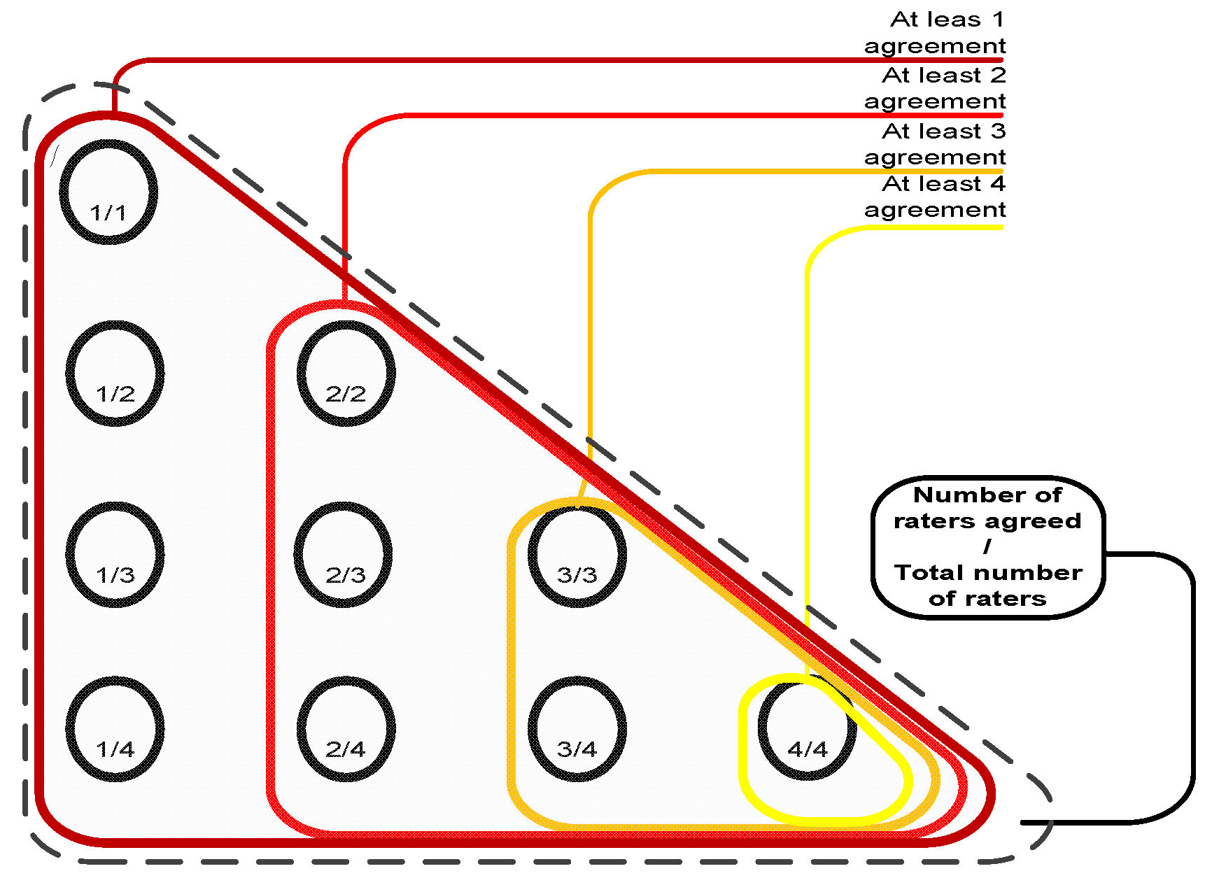
To evaluate the performance of the ensemble of classifiers and its agreement with the panel of experts, given the absence of ground truth (pathology or follow-ups are not available for the LIDC dataset), we consider the following reference truths: a) nodules rated by at least one radiologist b) nodules rated by at least two radiologists, and c) nodules rated by at least three radiologists–where the class label for each nodule in all cases is determined as the median of all ratings (up to four) (
Figure 5).
At this point in the study, we cannot evaluate the performance of the ensemble across individual radiologists since LIDC radiologists are anonymous even across nodules (radiologist 1 in one study is not necessary radiologist 1 in another study).
Figure 5.
Reference truths for the LIDC dataset.
Figure 5.
Reference truths for the LIDC dataset.
We will use the kappa statistic
k (8) to evaluate the degree to which the panel of experts agrees with the computer output with respect to each semantic characteristic:
where
p0 (Equation 9) stands for the observed agreement and
pe (Equation 10) stands for the agreement that would occur by chance:
where the agreement matrix A (Equation 11) consists of the number of correct classifications and misclassifications of every possible type (r = number of ratings):
For instance, when the panel’s rating for a nodule for spiculation was 3 and the ensemble of classifier rated the spiculation for the same nodule with 2, then the value in the third column, second row in the agreement matrix will be incremented by 1. The cells of the main diagonal are incremented only if the expert panel rating agrees with the CAD prediction. Given that we are predicting multiple ratings per semantic characteristic instead of just a binary rating, we also investigated the use of the weighted kappa statistic
kw that takes into consideration the significance of a particular type of misclassification and gives more weight
w (Equation 12) to a an error depending on how severe that error is:
for any two ratings
i and
j. The observed agreement
pow (Equation 13) and the agreement by chance
pew (Equation 14) are calculated as:
where the elements of the observed weighted proportions matrix
O and expected weighted proportions matrix
E are defined by (Equation 15) and (Equation 16), respectively:
4. Results
In this section we present the results of our proposed approach as follows. First, we present the accuracy results of Active-DECORATE with respect to balanced and unbalanced datasets, and “unseen” datasets - data that was not used by the ensemble to generate the classification rules. Second, we present the performance of Active-DECORATE in the variability index context in order to understand the effects of the nodule boundaries’ variability across radiologists. Third, we analyze the agreement between the panel of experts and the ensemble of classifiers both quantitatively using kappa statistics and visually using bar charts.
4.1. Accuracy results versus LIDC data subsets
By applying the active-DECORATE to the new LIDC dataset (
Table 4 and
Table 5), the classification accuracy was on average 70.48% (
Table 6) with an average number of iterations equal to 37 and average number of instances added at each iteration equal to 123. The results were substantially lower than on the previous available LIDC dataset (LIDC85–only 85 cases out of which only 60 cases were rated by at least one radiologist) for which the average accuracy was 88.62%.
Looking at the ratings distributions of the training datasets (nodules on which at least three radiologists agree) for the LIDC and LIDC85 datasets (
Table 5), we noticed that the distributions for the LIDC dataset were strongly skewed in the direction of one dominant class for almost each characteristic and therefore, produced unbalanced datasets when experimenting with our approach.
Table 4.
LIDC datasets overview; LIDC_B is a balanced data set.
Table 4.
LIDC datasets overview; LIDC_B is a balanced data set.
| | LIDC | LIDC85 | LIDC_B |
|---|
| Instances | 2,204 | 379 | 912 |
| Nodules | 914 | 149 | 542 |
| Cases/Patients | 207 | 60 | 179 |
Table 5.
Structure of the initial training data for all three datasets; L/U ratio represents the ratio between the labeled versus unlabeled data; ITI stands for initial training instances, N for the number of nodules and C for the number of cases.
Table 5.
Structure of the initial training data for all three datasets; L/U ratio represents the ratio between the labeled versus unlabeled data; ITI stands for initial training instances, N for the number of nodules and C for the number of cases.
| Dataset | LIDC | LIDC85 | LIDC_B |
|---|
| Characteristics | L/U ratio | #of ITI | N | C | L/U ratio | #of ITI | N | C | L/U ratio | #of ITI | N | C |
|---|
| Lobulation | 0.51 | 748 | 197 | 99 | 0.20 | 63 | 21 | 19 | 0.34 | 266 | 57 | 31 |
| Malignancy | 0.30 | 503 | 133 | 73 | 0.19 | 61 | 22 | 17 | 0.23 | 503 | 121 | 67 |
| Margin | 0.35 | 570 | 148 | 84 | 0.17 | 56 | 19 | 14 | 0.29 | 365 | 126 | 79 |
| Sphericity | 0.30 | 516 | 135 | 80 | 0.29 | 85 | 27 | 20 | 0.23 | 477 | 131 | 77 |
| Spiculation | 0.68 | 893 | 236 | 120 | 0.30 | 87 | 28 | 24 | 0.17 | 192 | 63 | 52 |
| Subtlety | 0.31 | 519 | 137 | 87 | 0.30 | 88 | 27 | 22 | 0.23 | 296 | 77 | 46 |
| Texture | 0.89 | 1040 | 277 | 123 | 0.46 | 120 | 35 | 24 | 0.23 | 173 | 36 | 11 |
| Average | 0.45 | 684 | 180 | 95 | 0.26 | 80 | 25 | 20 | 0.25 | 324 | 87 | 51 |
Table 6.
Classification accuracies of the ensemble of classifiers built using decision trees; the number of classifiers (Rsize) was set to 10 and number of artificially generated examples (Csize) to 1; #of ITR stands for number of iterations of Active-DECORATE, and #of IAL stands for number of instances added to the training data later (those that did not reach the confidence threshold).
| | LIDC (80% Confidence level) | LIDC85 (60% Confidence level) | LIDC_B (80% Confidence level) |
|---|
| Characteristics | #of ITR | #of IAL | Accuracy | #of ITR | #of IAL | Accuracy | #of ITR | #of IAL | Accuracy |
|---|
| Lobulation | 68 | 196 | 54.53% | 10 | 1 | 81.00% | 33 | 24 | 83.56% |
| Malignancy | 18 | 136 | 89.89% | 8 | 1 | 96.31% | 12 | 170 | 89.38% |
| Margin | 34 | 112 | 75.67% | 5 | 8 | 98.68% | 16 | 6 | 93.58% |
| Sphericity | 33 | 49 | 87.47% | 9 | 9 | 91.03% | 23 | 24 | 85.86% |
| Spiculation | 30 | 117 | 50.17% | 15 | 13 | 63.06% | 34 | 33 | 82.5% |
| Subtlety | 29 | 86 | 81.73% | 7 | 4 | 93.14% | 18 | 55 | 93.93% |
| Texture | 44 | 163 | 53.9% | 9 | 0 | 97.10% | 11 | 61 | 95.83% |
| Average | 36.6 | 122.7 | 70.48% | 9 | 5.14 | 88.62% | 21 | 53 | 89.23% |
To validate the effect of the unbalanced data on the accuracy of the classifier, we evaluated further the ensemble of classifier on another balanced dataset. The second subset (LIDC_B) was formed by randomly removing nodules from the most dominant class/rating such that the most dominant class has almost the same number of nodules as the second most dominant class.
Furthermore, when comparing our proposed approach with the traditional decision trees applied as single classifiers per characteristic, our approach notably outperforms the traditional approach by 24% to 45% accuracy, depending on the characteristics of the data subsets (
Table 7).
While all of the data instances were involved in the creation of both the decision trees and the ensemble from
Table 6 and
Table 7, we also wanted to test further the performance of our algorithm on “unseen” data. We reserved 10% of our data set to be completely unavailable (“unseen”) for the creation of the classifiers. This 10% was chosen to be similar to the entire data set with respect to levels of agreement and the distribution of semantic ratings. Further, if a patient had multiple nodules they were all included in the reserved 10%.
Table 7.
Classification accuracies of decision trees and an ensemble of decision trees on all datasets.
Table 7.
Classification accuracies of decision trees and an ensemble of decision trees on all datasets.
| | Decision trees | Ensemble approach |
|---|
| Characteristics | LIDC | LIDC85 | LIDC_B | LIDC | LIDC85 | LIDC_B |
|---|
| Lobulation | 49.4% | 27.44% | 38.52% | 54.53% | 81.00% | 83.56% |
| Malignancy | 39.11% | 42.22% | 38.88% | 89.89% | 96.31% | 89.38% |
| Margin | 38.56% | 35.36% | 39.56% | 75.67% | 98.68% | 93.58% |
| Sphericity | 34.21% | 36.15% | 32.21% | 87.47% | 91.03% | 85.86% |
| Spiculation | 59.43% | 36.15% | 59.16% | 50.17% | 63.06% | 82.5% |
| Subtlety | 38.11% | 38.79% | 39.51% | 81.73% | 93.14% | 93.93% |
| Texture | 66.74 | 53.56% | 60.42% | 53.9% | 97.10% | 95.83% |
| Average | 46.51% | 38.52% | 44.04% | 70.48% | 88.62% | 89.23% |
| Costs for ratings’ missclassifications | 1 | 2 | 3 | 4 | 5 |
|---|
| 1 | 0 | 0.5 | 1 | 1.5 | 2 |
| 2 | 0.5 | 0 | 0.5 | 1 | 1.5 |
| 3 | 1 | 0.5 | 0 | 0.5 | 1 |
| 4 | 1.5 | 1 | 0.5 | 0 | 0.5 |
| 5 | 2 | 1.5 | 1 | 0.5 | 0 |
Table 8.
Classification accuracies of Active-Decorate on original (90%) and reserved (10%) datasets.
Table 8.
Classification accuracies of Active-Decorate on original (90%) and reserved (10%) datasets.
| | Cross-validation on training data | Validation of testing data | |
|---|
| DT | AD | DT | AD | # of Patients | # of Nodules | # of Instances |
|---|
| Lobulation | 49.39% | 54.52% | 18.60% | 36.41% | 87 | 19 | 209 | |
| Malignancy | 39.44% | 90.65% | 31.00% | 35.75% | 84 | 19 | 213 | |
| Margin | 38.54% | 75.62% | 36.11% | 46.46% | 97 | 22 | 217 | |
| Sphericity | 33.89% | 86.65% | 14.26% | 57.49% | 84 | 19 | 226 | |
| Spiculation | 60.24% | 50.85% | 33.53% | 34.92% | 84 | 19 | 237 | |
| Subtlety | 38.87% | 83.35% | 25.14% | 15.03% | 82 | 18 | 248 | |
| Texture | 67.26% | 54.32% | 40.88% | 47.46% | 95 | 21 | 193 | |
| Average | 46.80% | 70.85% | 28.50% | 39.07% | 87 | 19 | 220 | |
Not surprisingly, when tested on a set of data that had never been viewed, both the single decision tree and our ensemble produced lower accuracies. However, one of the main features of the Active-DECORATE algorithm is its ability to dynamically adjust the ensemble when fed with newly available instances. In other words, the ensemble will not be generated just once, and then used in immutable form for classification of every new instance, but rather learn from every new instance it classifies, every time modifying the classification rules accordingly. Furthermore, associating different costs to different types of misclassifications (for example, misclassifying an instance as 3 when it is actually a 1 will receive a higher cost than when misclassifying it as 2 and a lower cost than when classifying it as 4), improves the results on the evaluation dataset by more than 20% (
Table 9). This is done by the application of a cost matrix to the misclassification matrix before evaluating accuracy. In our case, we used the following cost matrix:
Table 9.
Classification accuracies for original (90%) and reserved (10%) subsets after applying costs for degree of misclassification.
Table 9.
Classification accuracies for original (90%) and reserved (10%) subsets after applying costs for degree of misclassification.
| | AD (original data) | AD (original data) after applying cost | AD (reserved data) | AD (reserved data) after applying costs |
|---|
| Lobulation | 54.52% | 67.99% | 36.41% | 61.48% |
| Malignancy | 90.65% | 93.65% | 35.75% | 62.91% |
| Margin | 75.62% | 84.75% | 46.46% | 70.74% |
| Sphericity | 86.65% | 90.60% | 57.49% | 75.44% |
| Spiculation | 50.85% | 58.95% | 34.92% | 49.79% |
| Subtlety | 83.35% | 89.37% | 15.03% | 51.01% |
| Texture | 54.32% | 70.51% | 47.46% | 63.47% |
| Average | 70.85% | 79.40% | 39.07% | 62.12% |
Furthermore, we investigated the influence of the type of classifier on the accuracy of single classifiers and our proposed ensemble of classifiers approach.
Table 10 and
Table 11 show how single classifiers compare to ensembles, for both decision trees and support vector machines (In the case of the ensembles, decision trees and support vector machines serve as the base classifier). In average, the performance of an ensemble always exceeds the performance of a single classifier, and the performance of the support vector machine almost always exceeds the performance of the decision tree. In particular, the support vector machine does better on the reserved data set, meaning the support vector machine generalizes better than the decision tree.
Table 10.
Classification Accuracy of decision trees on full, original and reserved data sets (single classifier vs. ensemble of classifiers).
Table 10.
Classification Accuracy of decision trees on full, original and reserved data sets (single classifier vs. ensemble of classifiers).
| | DT | DT ensemble |
|---|
| full | original | reserved | full | original | reserved |
|---|
| Lobulation | 49.40% | 49.39% | 18.60% | 54.53% | 54.52% | 36.41% |
| Malignancy | 39.11% | 39.44% | 31.00% | 89.89% | 90.65% | 35.75% |
| Margin | 38.56% | 38.54% | 36.11% | 75.67% | 75.62% | 46.46% |
| Sphericity | 34.21% | 33.89% | 14.26% | 87.47% | 86.65% | 57.49% |
| Spiculation | 59.43% | 60.24% | 33.53% | 50.17% | 50.85% | 34.92% |
| Subtlety | 38.11% | 38.87% | 25.14% | 81.73% | 83.35% | 15.03% |
| Texture | 66.74% | 67.26% | 40.88% | 53.90% | 54.32% | 47.46% |
| Average | 46.51% | 46.80% | 28.50% | 70.48% | 70.85% | 39.07% |
Table 11.
Classification Accuracy of support vector machines on full, original and reserved data sets (single classifier vs. ensemble of classifiers).
Table 11.
Classification Accuracy of support vector machines on full, original and reserved data sets (single classifier vs. ensemble of classifiers).
| | SVM | SVM ensemble |
|---|
| | full | original | reserved | Full | original | reserved |
|---|
| Lobulation | 60.02% | 63% | 55.02% | 67.64% | 69.87% | 66.98% |
| Malignancy | 50.45% | 51.28% | 36.15% | 77.49% | 78.16% | 62.91% |
| Margin | 45.68% | 45.69% | 17.51% | 63.83% | 61.9% | 37.32% |
| Sphericity | 42.96% | 42.16% | 33.18% | 64.15% | 64.45% | 53.98% |
| Spiculation | 69.23% | 69.54% | 56.54% | 80.8% | 80.42% | 59.49% |
| Subtlety | 45.64% | 45.24% | 24.19% | 66.28% | 66.41% | 54.83% |
| Texture | 73.69% | 75.98% | 57.51% | 88.92% | 89.06% | 69.94% |
| Average | 55.38% | 55.78% | 40.01% | 72.73% | 72.89% | 57.92% |
4.2. Accuracy results versus variability index
The variability index was calculated for all LIDC nodules, specifically on those image instances that represented the slices containing the largest area of the nodule. The five number summaries for the distribution of the variability index had the following values: min = 0, first quartile (Q1) = 1.3165, median = 1.9111, third quartile (Q3) = 2.832, max = 85.5842. Then we calculated the five-number summary of the variability index for two subsets: the misclassified instances and the correctly classified instances with respect to each characteristic. Regardless of the characteristic, we learned that those instances with low variability index (<= 1.58) were correctly classified by the ensemble of classifiers and all those instances with high variability index (>= 4.95) were misclassified by the ensemble of classifiers. Given that variability index values greater than 5.12 (= Q3 + 1.5 × (Q3 – Q1)) indicate potential outliers in the boundary delineation, we conclude that the ensemble of classifiers is able to correctly classify instances with large variability in the nodule boundaries.
4.3. Ensemble of classifiers’ predictions versus expert panel agreement
Furthermore, we measured the agreement between the panel of experts and our ensemble of classifiers using both kappa and weighted kappa statistics for different levels of agreement. The results (
Table 12) show that higher levels of agreement yield higher kappa statistics. Furthermore, we noticed that weighted kappa statistics better captured the level of agreement than the non-weighted kappa statistic across different reference truths in the sense of being more consistent when going from one level of agreement to another. With the exception of spiculation and texture, the weighted kappa statistics for all the other five characteristics for the entire LIDC dataset showed that the ensemble of classifiers was in ‘moderate’ agreement or better (‘substantial’ or ‘almost perfect’) with the LIDC panel of experts when there were at least three radiologists who agreed on the semantic characteristics. Furthermore, when analyzing these five semantic characteristics with respect to the other two reference truths, we learned that the ensemble of classifiers was in ‘fair’ or ‘moderate’ agreement with the panel of experts.
Table 12.
Kappa statistics of different agreement level subsets of a new LIDC dataset.
Table 12.
Kappa statistics of different agreement level subsets of a new LIDC dataset.
| Agreement level | At least 3 | At least 2 | At least 1 |
|---|
| Characteristic | K | Kw | K | Kw | K | Kw |
|---|
| Lobulation | 0.10 | 0.4 | 0.06 | 0.27 | 0.06 | 0.24 |
| Malignancy | 0.82 | 0.89 | 0.38 | 0.63 | 0.28 | 0.55 |
| Margin | 0.45 | 0.59 | 0.28 | 0.39 | 0.22 | 0.29 |
| Sphericity | 0.7 | 0.78 | 0.3 | 0.46 | 0.23 | 0.4 |
| Spiculation | 0.05 | 0.27 | 0.04 | 0.24 | 0.04 | 0.22 |
| Subtlety | 0.51 | 0.66 | 0.35 | 0.48 | 0.26 | 0.39 |
| Texture | 0.03 | 0.2 | 0.05 | 0.19 | 0.05 | 0.18 |
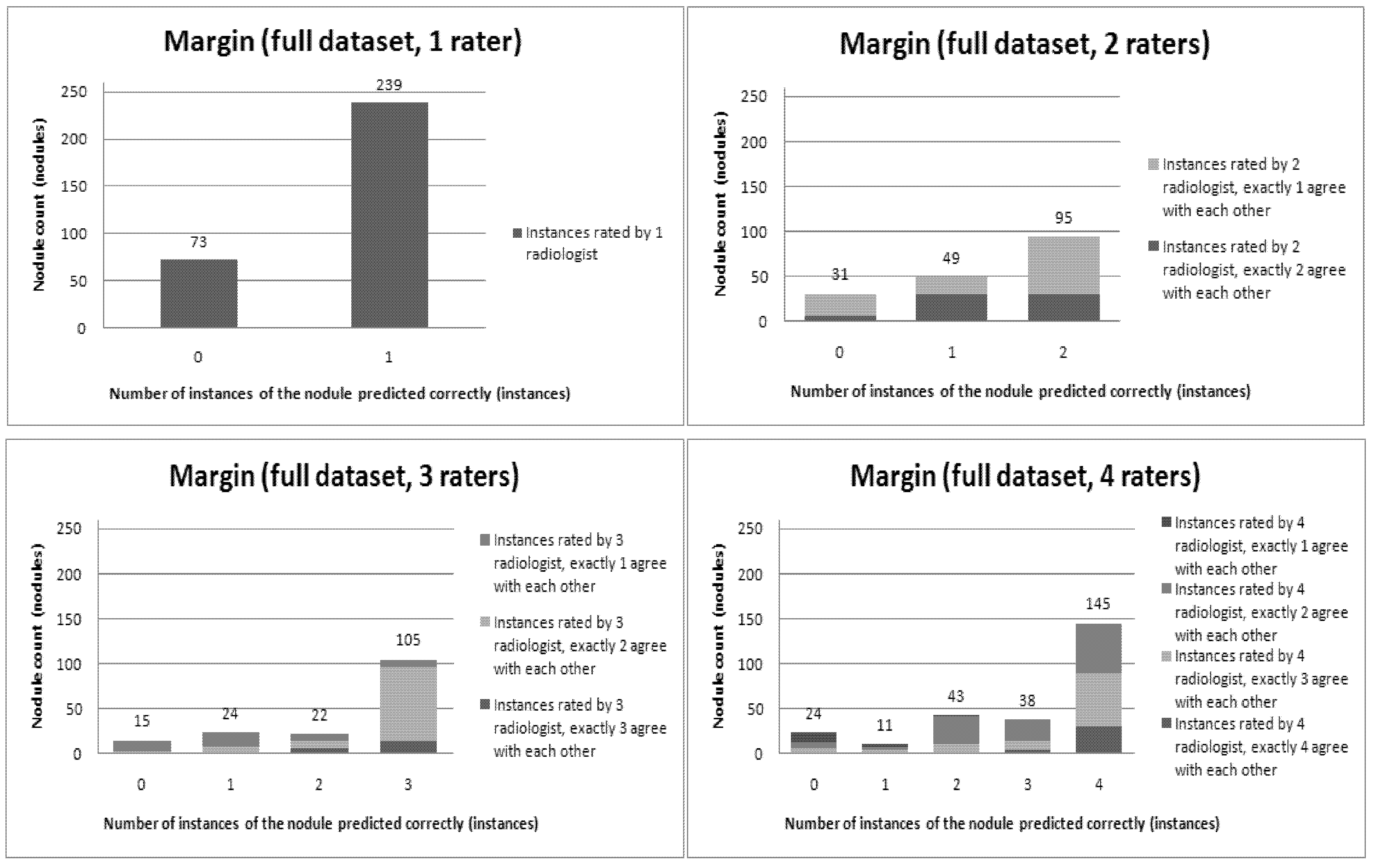
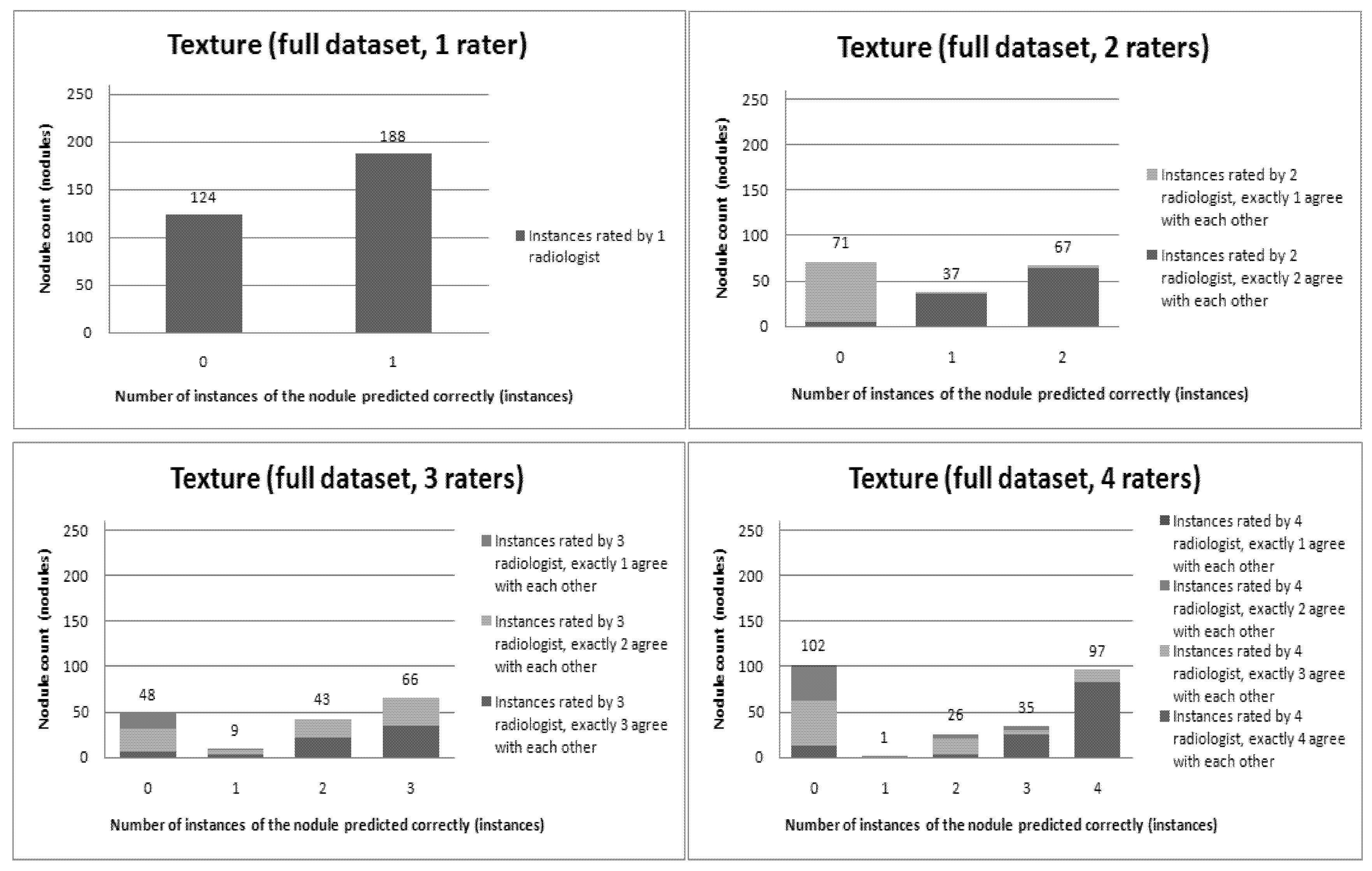
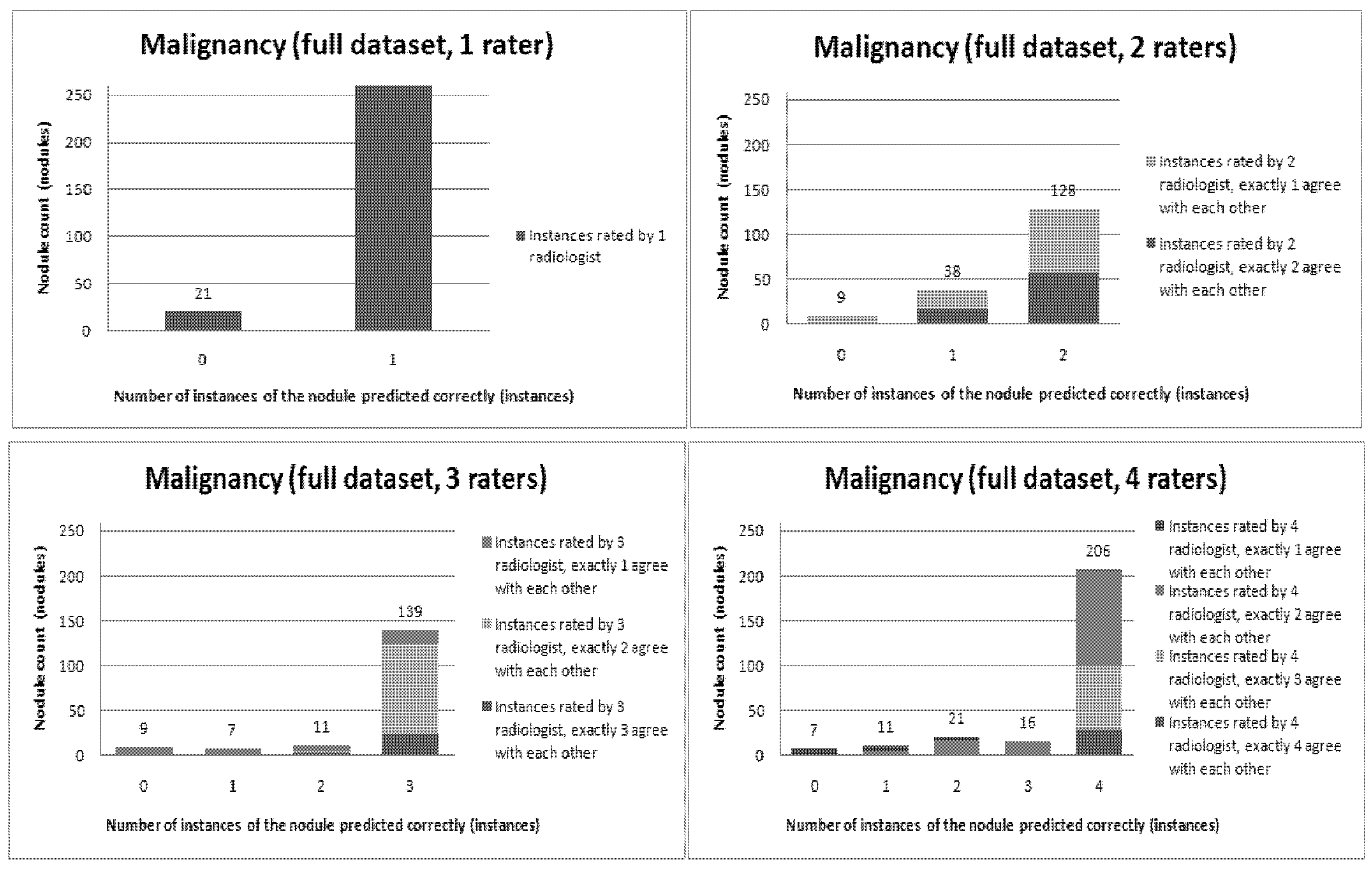
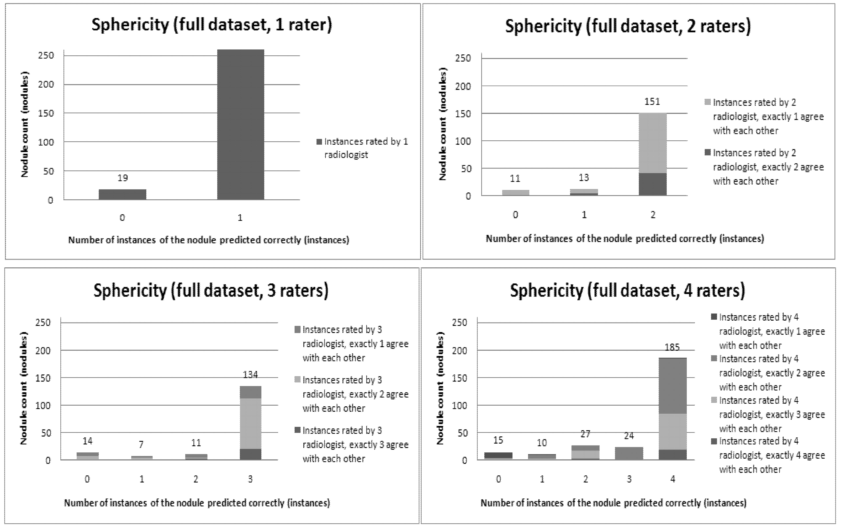
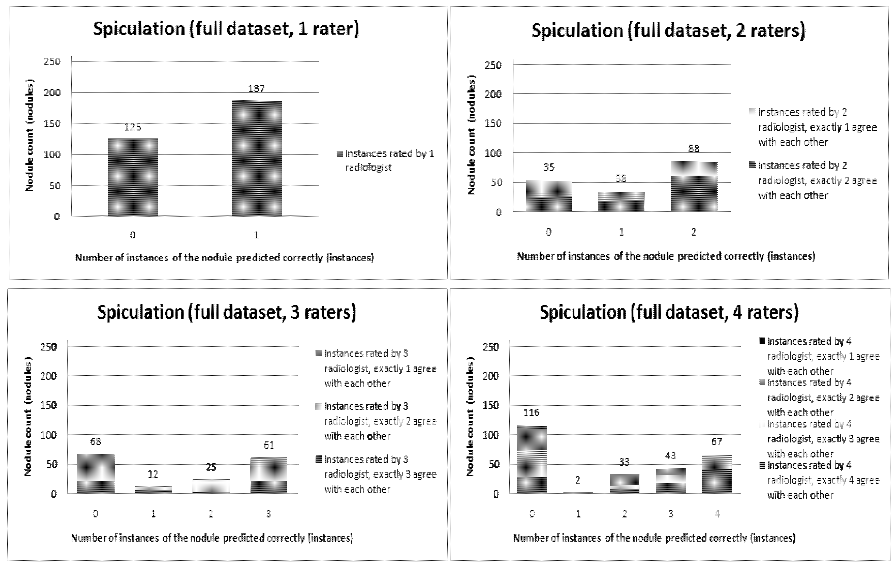
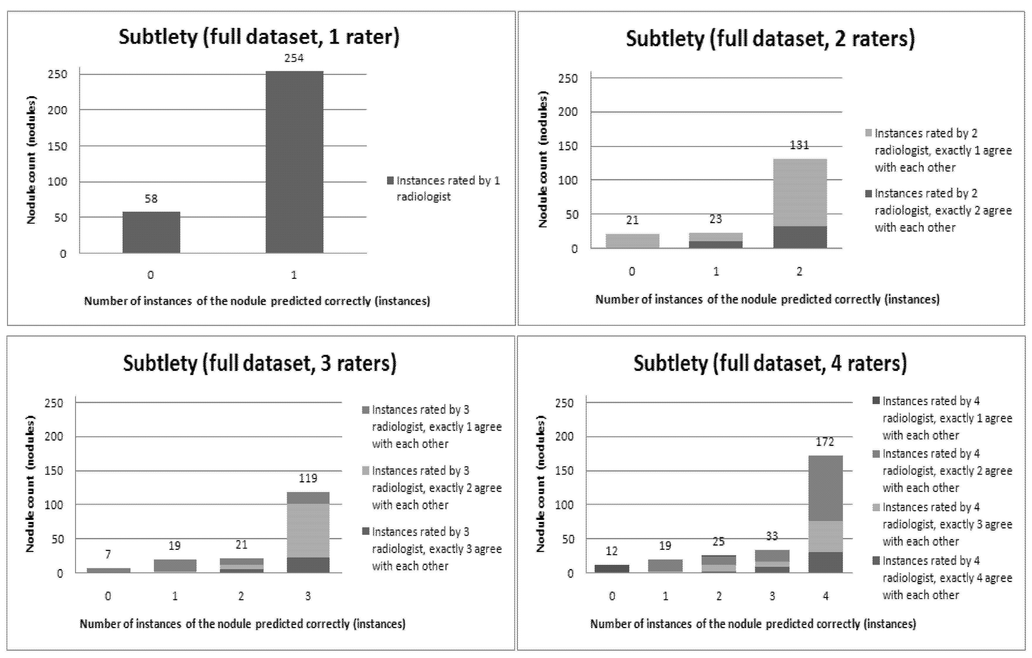
Figure 6,
Figure 7,
Figure 8,
Figure 9,
Figure 10,
Figure 11 and
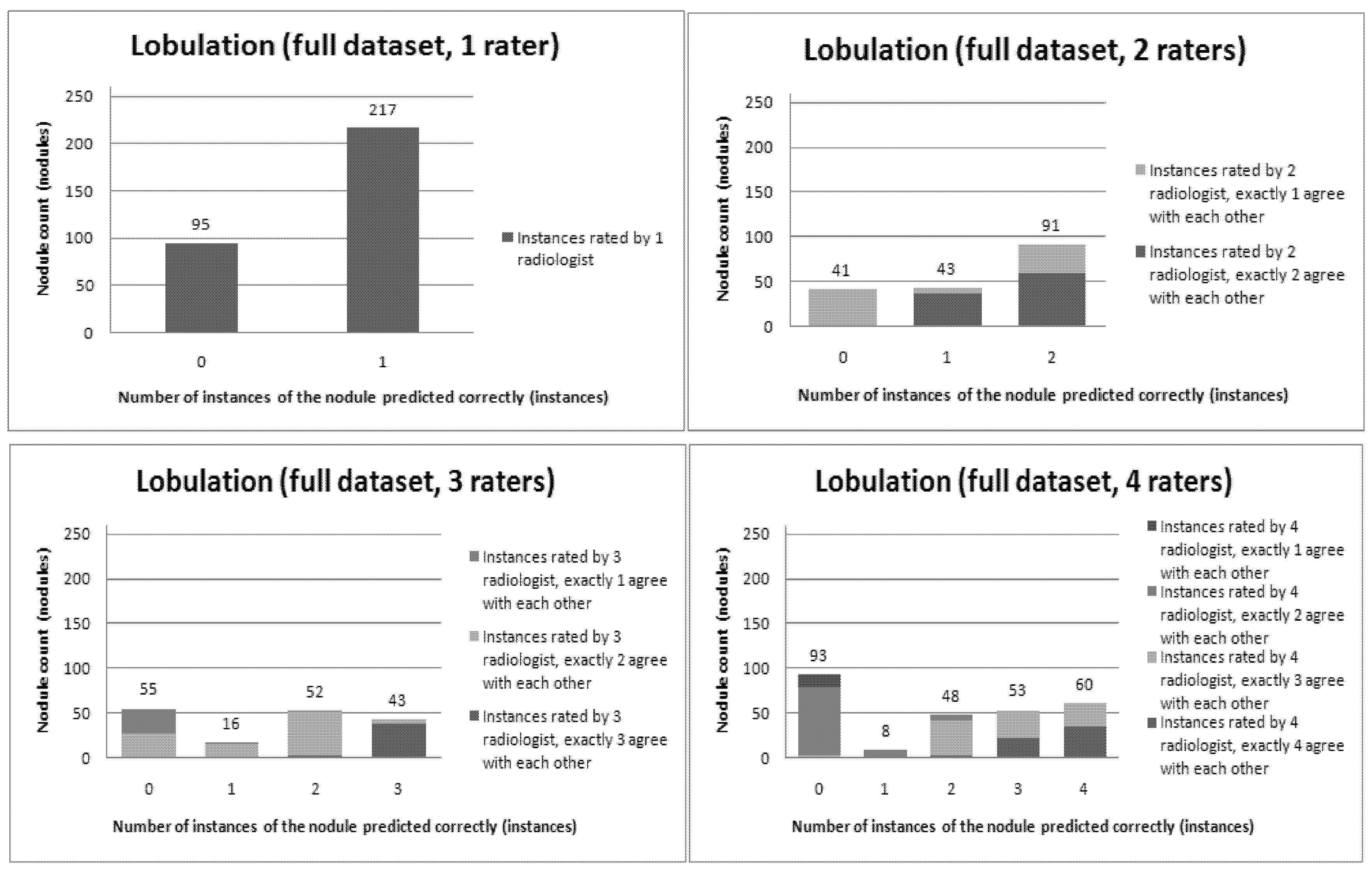
Figure 12 present a visual overview of the ensemble of classifiers’ agreement with the panel of experts’ opinions. In this visualization, we were interested not only in the “absolute” accuracy of the classifier, but also in how the classifier did with regard to rater disagreement. For each semantic characteristic, we have displayed four graphs. Each one of these graphs corresponds to a distinct number of raters. That is, we show one graph for nodules rated by one radiologist (upper left graph in each figure), one graph for nodules rated by two radiologists (upper right graph in each figure), one graph for nodules rated by three radiologists (lower left graph in each figure) and one graph for nodules rated by four radiologists (lower right graph in each figure). In each graph, we have a bar corresponding to the number of radiologists which our algorithm predicted correctly. (Thus the graphs with more radiologists have more bars.) The height of the bars shows how many nodules there were in each level of prediction success. Looking at just the height of these bars, we can see that our classifier’s success was quite good with respect to most of the semantic characteristics – these characteristics present very right-skewed distributions. Lobulation, spiculation and texture present more uniform distribution, meaning our classifier was less successful at predicting the radiologists’ labels. We present one further visualization in these graphs–each bar is gray-coded to indicate the radiologists’ level of agreement among themselves. (Thus, for example, the upper left graph, one radiologist, has no gray-coding, as a radiologist will always agree with himself.) This gray-coding allows us to see that the approach is much better at matching radiologists when the radiologists agree with themselves. While this, in itself, is not surprising, it does reveal that for the troublesome characteristics (lobulation, spiculation and texture) the algorithm does a very good job when we look only at higher levels of radiological agreement.
Figure 6.
Visual overview of the ensemble of classifiers’ agreement with the panel of experts’ opinions (Lobulation).
Figure 6.
Visual overview of the ensemble of classifiers’ agreement with the panel of experts’ opinions (Lobulation).
Figure 7.
Visual overview of the ensemble of classifiers’ agreement with the panel of experts’ opinions (Malignancy).
Figure 7.
Visual overview of the ensemble of classifiers’ agreement with the panel of experts’ opinions (Malignancy).
Figure 8.
Visual overview of the ensemble of classifiers’ agreement with the panel of experts’ opinions (Margin).
Figure 8.
Visual overview of the ensemble of classifiers’ agreement with the panel of experts’ opinions (Margin).
Figure 9.
Visual overview of the ensemble of classifiers’ agreement with the panel of experts’ opinions (Sphericity).
Figure 9.
Visual overview of the ensemble of classifiers’ agreement with the panel of experts’ opinions (Sphericity).
Figure 10.
Visual overview of the ensemble of classifiers’ agreement with the panel of experts’ opinions (Spiculation).
Figure 10.
Visual overview of the ensemble of classifiers’ agreement with the panel of experts’ opinions (Spiculation).
Figure 11.
Visual overview of the ensemble of classifiers’ agreement with the panel of experts’ opinions (Subtlety).
Figure 11.
Visual overview of the ensemble of classifiers’ agreement with the panel of experts’ opinions (Subtlety).
Figure 12.
Visual overview of the ensemble of classifiers’ agreement with the panel of experts’ opinions (Texture).
Figure 12.
Visual overview of the ensemble of classifiers’ agreement with the panel of experts’ opinions (Texture).
5. Conclusions
In this paper, we presented a semi-supervised learning approach for predicting radiologists’ interpretations of lung nodule characteristics in CT scans based on low-level image features. Our results show that using nodules with a high level of agreement as initially labeled data and automatically labeling the data on which disagreement exists, the proposed approach can correctly predict 70% of the instances contained in the dataset. The performance represents a 24% overall improvement in accuracy in comparison with the result produced by the classification of the dataset by classic decision trees. Furthermore, we have shown that using balanced datasets, our approach increases its prediction accuracy by 45% over the classic decision trees. When measuring the agreement between our computer-aided diagnostic characterization approach and the panel of experts, we learned that there is a moderate or better agreement between the two when there is a higher consensus among the radiologists on the panel and at least a ‘fair’ agreement when the opinions among radiologists vary within the panel. We have also found that high disagreement in the boundary delineation of the nodules also has a significant effect on the performance of the ensemble of classifiers.
In terms of future work, we plan to explore further (1) different classifiers and their performance with respect to the variability index in the expectation of improving our performance, (2) 3D features instead of 2D features so that we can include all the pixels in a nodule without drastically increasing the image feature vector size, and (3) integration of the imaging acquisition parameters in the ensemble of classifiers so that our algorithm will be stable in the face of images obtained from different models of imaging equipment. In the long run, it is our aim to use the proposed approach to measure the level of inter-radiologist variability reduction by supplying our CAD characterization approach in between the first and second pass of radiological interpretation.


 is the probability of example x belonging to class yk according to the classifier Ci. The probability given by Equation 1 is used to identify the nodules predicted with high confidence.
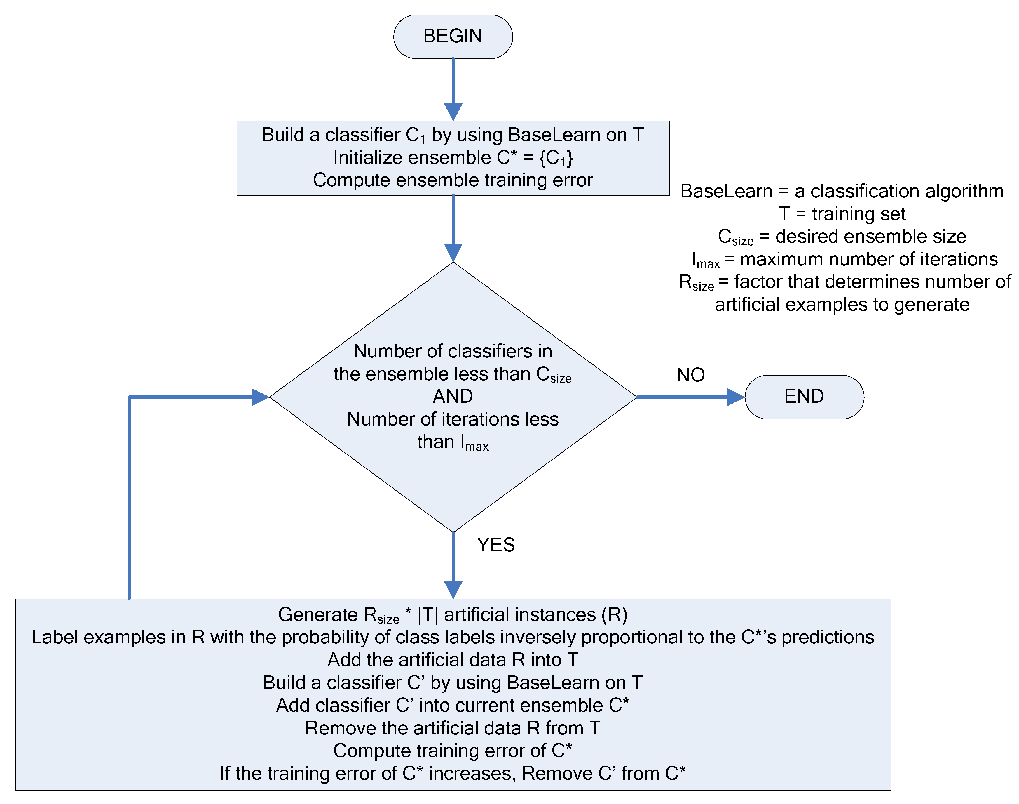


 are the mean and variance of row and column.


