Image Similarity to Improve the Classification of Breast Cancer Images

US Army Research Laboratory, 2800 Powder Mill Rd, Adelphi, MD 20783, USA
Algorithms 2009, 2(4), 1503-1525; https://doi.org/10.3390/a2041503
Submission received: 12 October 2009
/
Revised: 20 November 2009
/
Accepted: 25 November 2009
/
Published: 1 December 2009
(This article belongs to the Special Issue Machine Learning for Medical Imaging)
Abstract
:Techniques in image similarity can be used to improve the classification of breast cancer images. Breast cancer images in the mammogram modality have an abundance of non-cancerous structures that are similar to cancer, which make classification of images as containing cancer especially difficult to work with. Only the cancerous part of the image is relevant, so the techniques must learn to recognize cancer in noisy mammograms and extract features from that cancer to appropriately classify images. There are also many types or classes of cancer with different characteristics over which the system must work. Mammograms come in sets of four, two images of each breast, which enables comparison of the left and right breast images to help determine relevant features and remove irrelevant features. In this work, image feature clustering is done to reduce the noise and the feature space, and the results are used in a distance function that uses a learned threshold in order to produce a classification. The threshold parameter of the distance function is learned simultaneously with the underlying clustering and then integrated to produce an agglomeration that is relevant to the images. This technique can diagnose breast cancer more accurately than commercial systems and other published results.
1. Introduction
A technique that radiologists use to diagnose breast cancer involves first finding suspicious sites in the mammograms and then comparing the left and right breasts to reduce the number of false positives. The symmetry of the human body is utilized to increase the accuracy of the diagnosis through visual registration of the mammograms. This technique is emulated by combining both computer vision and learning techniques, attempting to capture the diagnosis of the radiologist. Therefore this work is motivated not only by computer science theory and technique, but also by domain-specific knowledge and theory. These ideas were verified through an approach that has been completed with surprisingly good results at diagnosing breast cancer. It is hoped that this work will improve techniques in image similarity and classification, as well as provide insights into medical imaging and especially into the imaging, diagnosis, and classification of breast cancer.
Breast cancer remains a leading cause of cancer deaths among women in many parts of the world. In the United States alone, over forty thousand women die of the disease each year [1]. Mammography is currently the most effective method for early detection of breast cancer [2], and example mammograms are shown in Figure 1. Computer-aided detection (CAD) of mammograms could be used to avoid these missed diagnoses, and has been shown to increase the number of cancers detected by more than nineteen percent [3], so there is hope that improving techniques in computerized detection of breast cancer could significantly improve the lives of women across the globe. Studies have shown that CAD can improve the search and detection of cancer associated with micro-calcification clusters [4,5], but cancers associated with masses are often considered to be false positives in the clinical environment [6,7]. Poor performance is caused by high false-positive rates [8] and the use of only one view [9]. The benefit of using CAD systems are still being tested [10,11], and new CAD schemes are being developed [12,13,14,15,16,17,18,19,20,21,22,23,24,25,26]. Asymmetry, which consists of a comparison of the left and right breast images [27], is a technique that could be used to significantly improve the results. An automated prescreening system only classifies a mammogram as either normal or suspicious, while CAD picks out specific points as cancerous [28]. One of the most challenging problems with prescreening is the lack of sensitive algorithms for the detection of asymmetry [29]. Image similarity methods can capture the asymmetry properties, and then improve both CAD and prescreening of breast cancer.
Contextual and spatial comparisons can be combined to determine image similarity, which has been often utilized in image databases [30,31,32,33]. Medical image databases have also used image similarity, ranging from rule-based systems for chest radiographs [34] to anatomical structure matching for 3-D MR images [35] to learning techniques [36]. This work applies image similarity concepts to the problem of detecting breast cancer for CAD in mammograms.
Detecting breast cancer in mammograms is challenging because the cancerous structures have many features in common with normal breast tissue. This means that a high number of false positives or false negatives are possible. Asymmetry can be used to help reduce the number of false positives so that true positives are more obvious. Previous work utilizing asymmetry has used wavelets or structural clues to detect asymmetry with correct results as often as 77% of the time [27,37]. Additional work has focused on bilateral or temporal subtraction, which is the attempt to subtract one breast image from the other [38,39]. This approach is hampered by the necessity of exact registration and the natural asymmetry of the breasts. Bilateral subtraction tries to utilize the multiple images taken with the same machine by the same technician and analyzed using the same process in an effort to reduce the systematic differences that can be introduced. Developing ways to better utilize asymmetry is consistent with a philosophy of trying to use methods that can capture measures deemed important by doctors thereby building upon their knowledge base, instead of trying to supplant it. However, measuring asymmetry involves registration and comparing multiple images, and thus it is a more complicated process.
Figure 1.
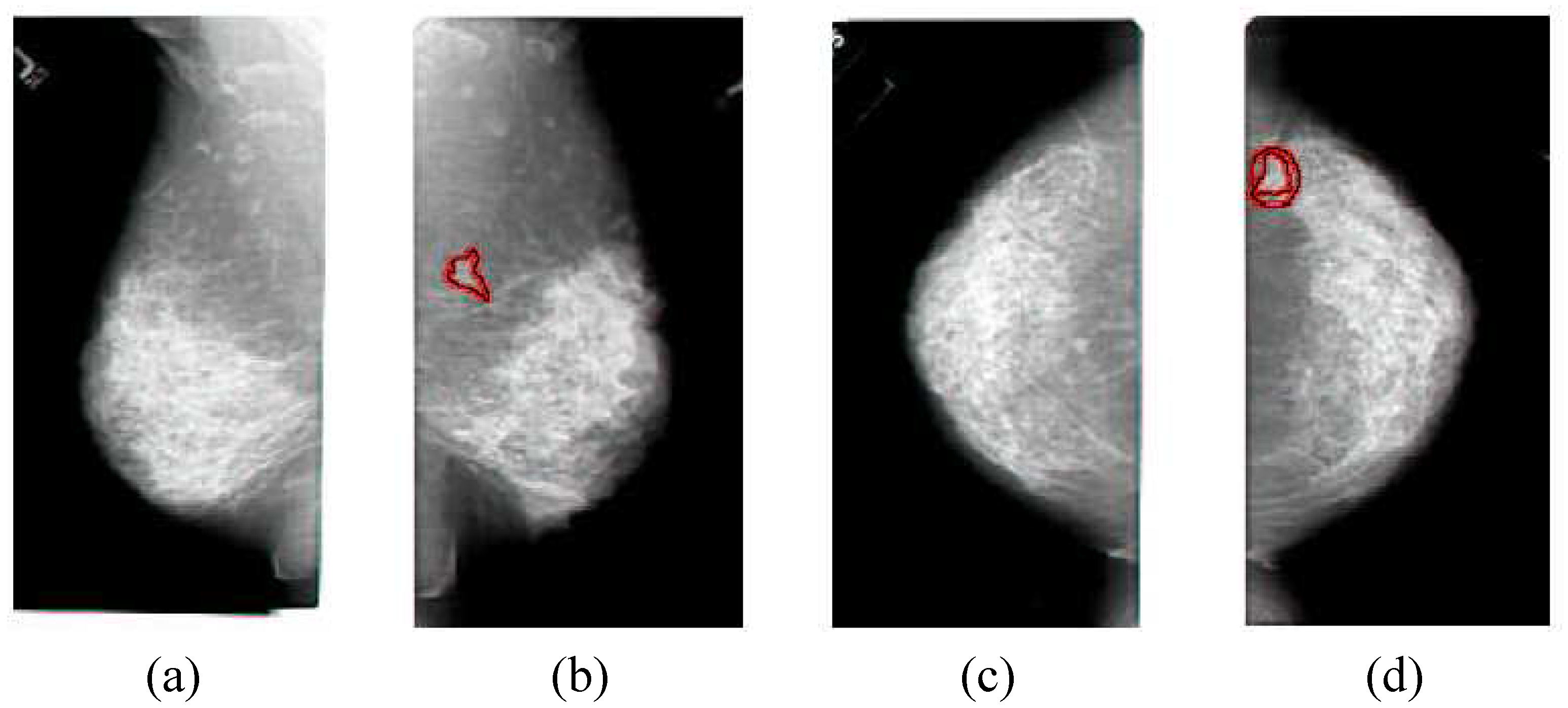
The typical set of four images that make up a mammogram, the side view of the left breast in (a), the side view of the right breast in (b), the top view of the left breast in (c), the top view of the right breast in (d). The cancerous areas are outlined in red. Since the images come in sets, the non-cancerous cases are examples of similar images, while the cancerous cases are examples of dissimilar images, and these examples can be used to determine image similarity. Note that the textures of the cancer are very similar to non-cancerous areas, which is why image comparisons are so important in the analysis of mammograms. Also note that the cancer is apparent in both images of the same breast, which provides additional information for the analysis. This image set was correctly classified by the method described in Section 3.
Figure 1.
The typical set of four images that make up a mammogram, the side view of the left breast in (a), the side view of the right breast in (b), the top view of the left breast in (c), the top view of the right breast in (d). The cancerous areas are outlined in red. Since the images come in sets, the non-cancerous cases are examples of similar images, while the cancerous cases are examples of dissimilar images, and these examples can be used to determine image similarity. Note that the textures of the cancer are very similar to non-cancerous areas, which is why image comparisons are so important in the analysis of mammograms. Also note that the cancer is apparent in both images of the same breast, which provides additional information for the analysis. This image set was correctly classified by the method described in Section 3.

Registration is the matching of points, pixels, or structures in one image to another image. Registration of mammograms is difficult because mammograms are projections of compressed three-dimensional structures. Primary sources of registration errors are differences in positioning and compression, which manifests itself in visually different images. The problem is more complex because the breast is elastic and subject to compression. Additional sources of difficulty include the lack of clearly defined landmarks and the normal variations between breasts. Strictly speaking, precise mammogram registration is intractable. However, an approximate solution is possible [40]. Warping techniques have been used [41], as well as statistical models [42] or mutual information as a basis for registration [43]. The technique advanced in this paper learns image comparison models based upon a clustering that encapsulates an approximate registration and uses them to compare the mammograms of the left and right breasts. This also avoids direct registration when measuring the image similarity.
The rest of this paper is organized as follows. Section 2 describes mammogram images and feature extraction from mammograms. Section 3 details the approach taken as an initial data exploration and classification approach, and the development of a distance function. Section 4 describes the improvement to CAD approaches through the inclusion of similarity. The conclusion is in Section 5.
2. Mammogram Image Description and Feature Extraction
A mammogram is an x-ray exam of the breast. It is used to detect and diagnose breast disease, both in women who have no breast complaints or symptoms and in women who have breast cancer symptoms (such as a lump). The special type of x-ray machine used for the breasts is different than for other parts of the body. This type of machine produces x-rays that do not penetrate tissue as easily as that used for routine chest films or x-rays of the arms or legs, and gives a better image of variations in tissue density. For a mammogram, the breast is squeezed between two plastic plates attached to the mammogram machine unit in order to spread the tissue apart. This squeezing or compression ensures that the calibration will be accurate, that there will be very little movement so the image is sharper, and that the exam can be done with a lower x-ray dose. However, it also makes 3-D reconstruction of the breast structure much more difficult.
Mammography produces a black and white image of the breast tissue on a large sheet of film which is interpreted by a radiologist. The appearance of the breast on a mammogram varies a great deal from woman to woman. Some breast cancers produce changes in the mammogram that are difficult to notice. Breast cancer takes years to develop. Early in the disease, most breast cancers have none of the obvious symptoms like lumps. When breast cancer is detected in a localized stage and when it has not spread to the lymph nodes, the five year survival rate is 98% [1]. If the cancer has spread to the auxiliary lymph nodes, the rate drops to 80% [1]. If the cancer has metastasized to distant organs such as the lungs, bone marrow, liver, or brain, the five-year survival rate is only 26% [1]. A screening mammogram is an x-ray exam of the breast in a woman who has no symptoms and usually takes two x-ray images of each breast, as is shown in Figure 1. The goal of a screening mammogram is to find cancer when it is still too small to be felt by a woman or her doctor. Finding small breast cancers early by a screening mammogram greatly improves a woman’s chance for successful treatment and survival.
Breasts vary in density, which affects the appearance of the breast in mammograms. Examples of the variations are shown in Figure 2. The American College of Radiology (ACR) Breast Imaging Reporting and Data System (BIRADS) characterizes these as ranging from 1-4, with 4 being the most dense. A dense breast presents more non-cancerous structures on a mammogram that can obscure a mass.
The majority of work on feature analysis of mammograms has been through CAD efforts, focusing on determining the contextual similarity to cancer and finding abnormalities in a local area of a single image [44,45]. The primary methods used range from filters to wavelets to learning methods. In this context, filters are equivalent to shapes that are searched for in an image. Wavelets are the result of applying a transform to the image, and learning methods try to apply prior knowledge to combine a set of low-level image features like pixel intensities into an accurate classification. Problems arise in using filter methods [44] because of the range of sizes and morphologies for breast cancer, as well as the difficulty in differentiating cancerous from non-cancerous structures. The size range problem has been addressed by using multi-scale models [45]. Multiple types of filters must be used to handle the variation in the morphology of various cancers. Similar issues affect wavelet methods, although their use has led to reported good results [46] with the size range issue being improved through the use of a wavelet pyramid [47]. Learning techniques have included support vector machines [48] and neural networks [46].
Figure 2.
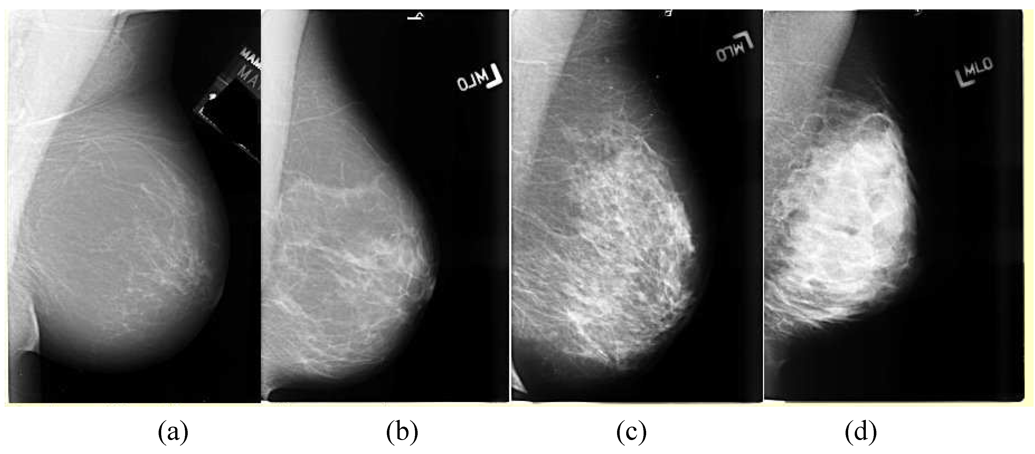
The variations in density a mammogram, the least dense in (a) being characterized as mostly fat to the very dense breast in (d). The American College of Radiology (ACR) Breast Imaging Reporting and Data System (BIRADS) characterizes these as ranging from 1–4, with 4 being the most dense.
Figure 2.
The variations in density a mammogram, the least dense in (a) being characterized as mostly fat to the very dense breast in (d). The American College of Radiology (ACR) Breast Imaging Reporting and Data System (BIRADS) characterizes these as ranging from 1–4, with 4 being the most dense.

Our analysis starts with CAD prompts to find the contextually similar suspicious points that could be cancers in the mammograms. The CAD technique highlights the areas of the image that have bright cores, a characteristic of spiculated lesions as shown in Figure 3a. The filter calculates the percent of the pixels in the outer ring that are less bright than the least bright of the pixels in the inner disk to produce a suspiciousness value, and an example is given in Figure 3b. This suspiciousness value represents the degree to which the surrounding region of a point radially decreases in intensity, and is done over several sizes. This results in focusing on the bright central core of the cancer and ignoring the radiating lines of spiculation. A second filter can be used to detect the radiating lines of spiculation, as shown in Figure 3c, but a combined filter shown in Figure 3d that detects both the cores and the spiculation could improve the performance, especially if the relative weighting of the measurements is learned on an appropriate data set.
Figure 3.
(a) Mammographic image of a spiculated lesion. (b) AFUM filter. (c) Cosine Gabor filter. (d) Combined filter.
Figure 3.
(a) Mammographic image of a spiculated lesion. (b) AFUM filter. (c) Cosine Gabor filter. (d) Combined filter.

The CAD suspiciousness calculation is performed at each pixel location (x,y) in the images. The minimum intensity Imin within r1 is found, and then the fraction of pixels between r1 and r2 with intensities less than Imin is calculated. This yields the fraction under the minimum (FUM) for one set of r1 and r2. Keeping r1 – r2 = b constant and averaging the FUM over a range of r1 determines the average fraction under the minimum (AFUM) [31]. The AFUM is then considered to be a suspiciousness value, and represents the extent to which the surrounding region of a point radially decreases in intensity. The CAD prompt output is a set of these suspicious points that are above a certain threshold. Since this is done over a range of sizes, it can respond to cancers of different sizes. This focuses on the bright central core of the cancer and ignores the radiating lines of spiculation. The distribution of these features on a mammogram is shown in Figure 4.
Figure 4.
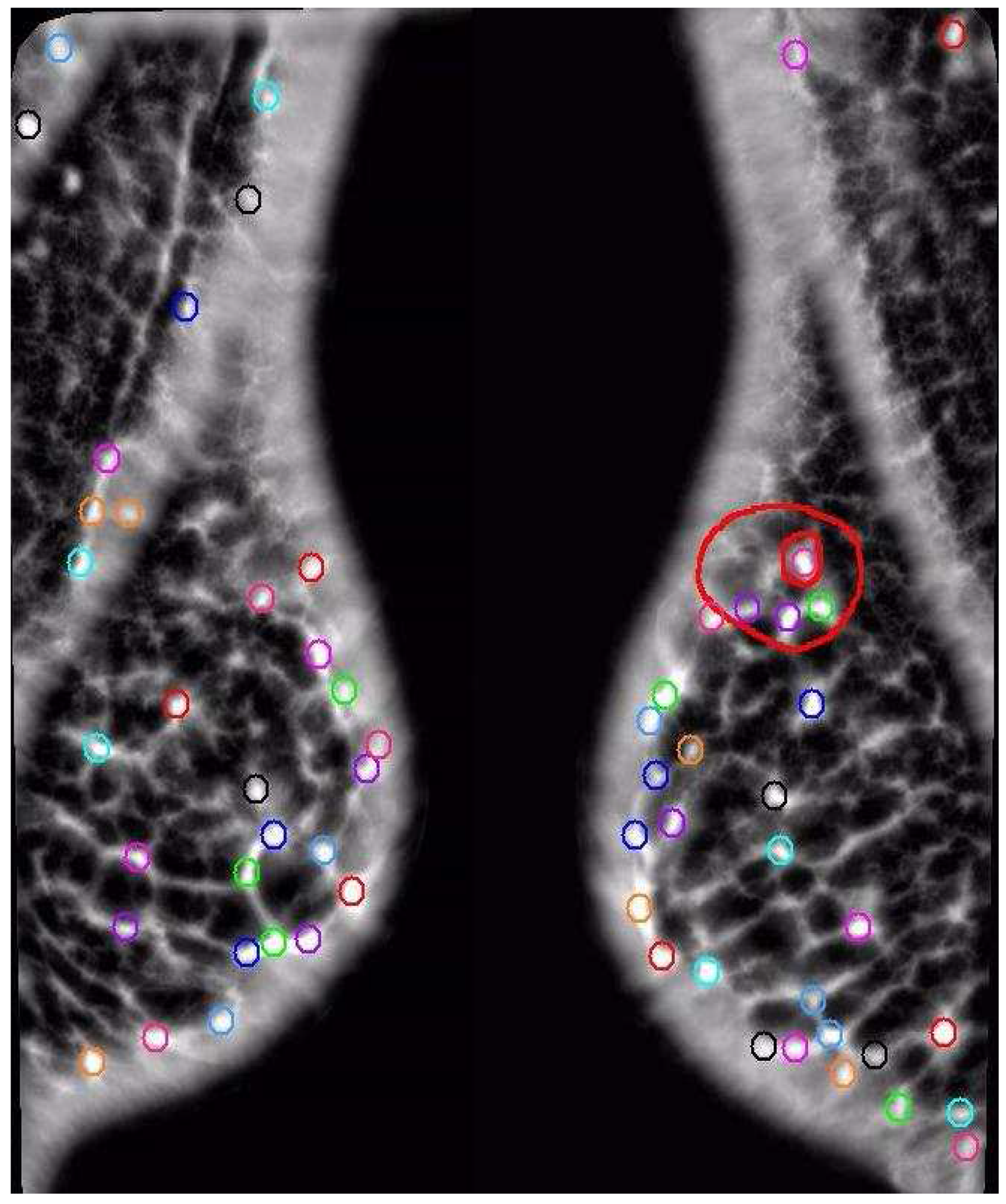
The distribution of the AFUM features on a mammogram are shown as small circles, while the larger oval shapes are hand-drawn annotations by a radiologist of the cancer. Note that the feature does find a cancer, but there are many false positives.
Figure 4.
The distribution of the AFUM features on a mammogram are shown as small circles, while the larger oval shapes are hand-drawn annotations by a radiologist of the cancer. Note that the feature does find a cancer, but there are many false positives.

Features with a high suspiciousness value have a higher chance of corresponding to an occurrence of cancer. The centroid of each local maxima in the filtered image is initially marked as a candidate feature site with its suspiciousness value. This collection of sites is then sorted in decreasing order of suspicion. All suspicious sites that are closer than 5 mm from a more suspicious site are removed to prevent multiple reporting of the same site. This yields a set of potential feature sites that can be analyzed.
A further improvement might be possible by first transforming the data before filtering, such as applying wavelet analysis to the images before simply thresholding or applying the filter. This has been successfully attempted previously [27] with good results. However, an optimal solution would first combine all of the various filtering and transform methods which create meaningful suspicious points, and then learn an effective analysis from them. This is similar to the effective combination of weak classifiers into a single strong classifier through ensemble learning methods like boosting, which has been successfully used before in tumor classification [49]. Many of the images like mammograms come in pairs, so they form a set that should be very similar. If one of the pair contains cancer and the other does not, then that pair should be different. Thus, the mammogram image set provides both positive and negative examples to build on for image similarity classification.
Figure 5.
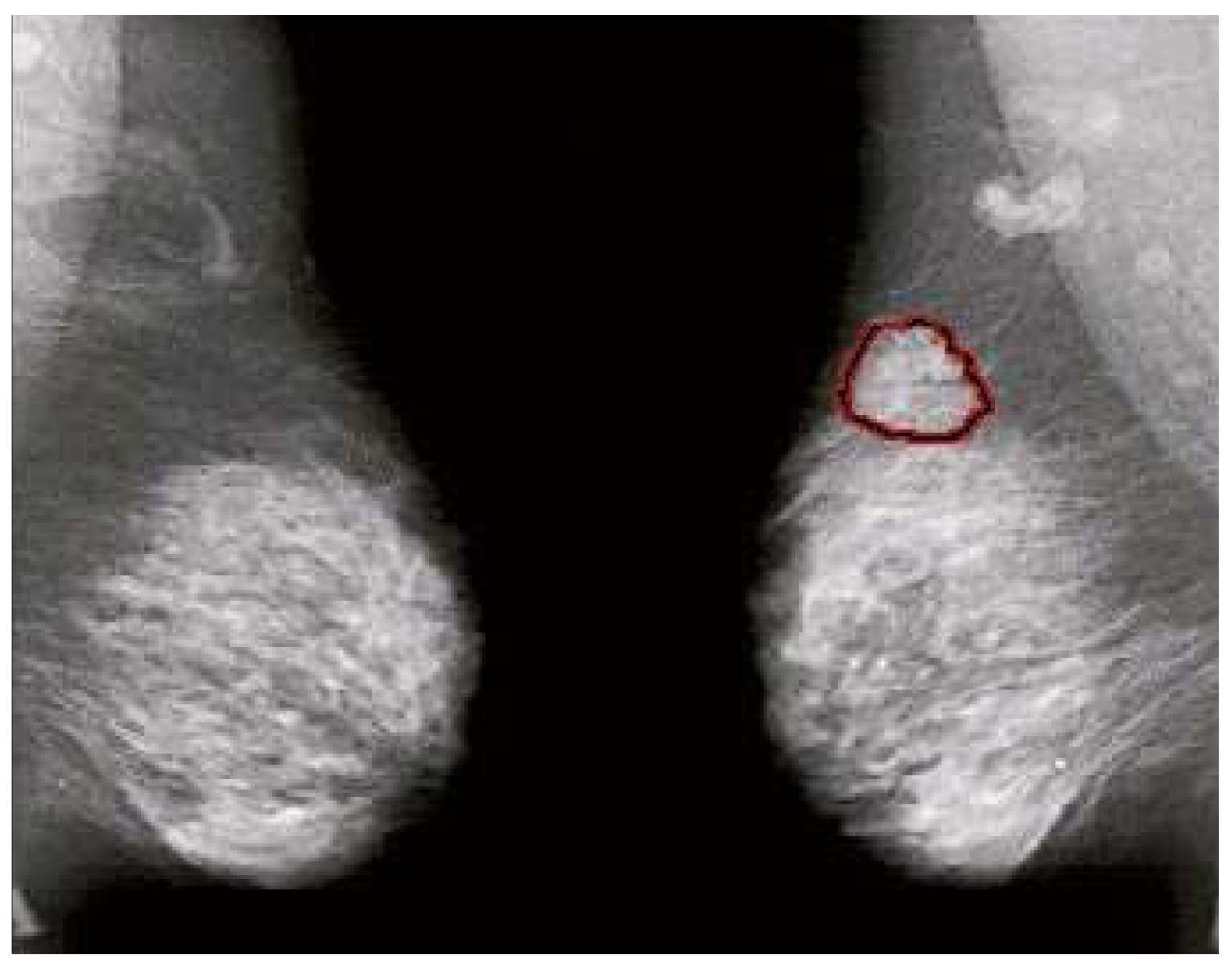
Mammograms of left and right breasts with cancerous area outlined. The similarity of texture between cancerous and normal tissue makes asymmetry an important tool in cancer detection.
Figure 5.
Mammograms of left and right breasts with cancerous area outlined. The similarity of texture between cancerous and normal tissue makes asymmetry an important tool in cancer detection.

3. Breast Cancer Image Classification
An effort was made to provide image classifications and to develop a distance function for CAD of medical images as well as to explore the properties of the dataset. This initial approach utilizes filtering followed by spatial symmetry analysis using a variant of supervised clustering to determine an overall measure of similarity by combining the contextual similarity of the filtering with the spatial similarity of the analysis. This can be a useful measure for diagnosing mammograms (or for pre-screening) since only an overall determination of cancer or no cancer is required. A secondary goal of our work is to determine the importance of similarity or asymmetry in the computer analysis of mammograms. Figure 5 shows why spatial asymmetry is important in finding cancers in mammograms since we see that the texture and appearance of cancer are both very similar to the texture and appearance of normal tissue in the breast. Our analysis starts with filtering to find the contextually similar suspicious points that could be cancers in the mammograms. The AFUM filter was used, which highlights the areas of the image that have bright cores, a characteristic of spiculated lesions, and is shown in Figure 3b. The filter results are used to rank the output and only the top thirty-two are kept. Although it may not be the optimal choice of filtering, the spatial analysis can be applied to any technique that can rank the suspiciousness of areas. The number of points returned by the filtering step is one of the variables that were learned in optimizing the analysis. Alternatively, a threshold on the suspiciousness value could have been used instead of taking the top few. However, the top few were chosen in order to try to be insensitive to image processing choices. The filter results varied significantly from image to image, which might have biased the analysis if thresholds were used.
Several techniques were developed to aid in the development of an improved distance function for the classification of medical images. We used clustering as a basis for determining image similarity, but there were several changes that had to be made to the technique to adapt it to the application. First, instead of utilizing cluster centers as the main descriptor of the clustering, we used both linear separators in the original feature space as well as hyper-volumes to describe the clusters. Second, we adapted the clustering method to use supervised learning instead of minimizing an objective function. Third, we incorporated the clusters into several distance functions, the parameters of which were learned simultaneously with the cluster definitions to produce an image similarity classification technique. Fourth, since the importance of correct classification of the cancerous cases is much more important than the non-cancerous cases, the associated weighting of the cancerous cases was varied, and we evaluated the performance of various weightings. The algorithm is composed of the following steps:
- Extract K points from both of the images using an AFUM filter.
- Assign each point to the appropriate cluster defined by the parameters P.
- Apply the distance function over the clusters.
- Determine the error function from the supervised cases.
- Adjust the cluster and distance function parameters P.
- Repeat Steps 2 through 5 until the error is minimized.
This produces a clustering in the feature space that is independent of the classification and can be used to learn about the image properties. It also produces a threshold for the distance function simultaneously with the cluster parameters. The details on step 1 were given in Section 2, while the details on the clustering are in Section 3.1, the details on the supervised learning in Section 3.2, and the distance function in Section 3.3.
3.1. Separators and Hyper-Volumes
The adaptation of clustering to use separators and hyper-volumes instead of cluster centers was motivated by a desire to minimize the number of parameters required in order to maximize the generalizability of the technique from the training data to the actual test data and thus to real applications. Creating two clusters requires two d-dimensional cluster centers, or 2d parameters like P = (x1, y1, z1, x2, y2, z2), while using a separator plane requires a maximum of d parameters like P = (a, b, c) and can be described in as few as one parameter in special cases like P = (a). Four clusters can be described using as few as two separator planes, greatly reducing the number of parameters required to describe the clustering. However, eliminating parameters can change the final clustering. There is a tradeoff between the number of parameters and the flexibility of the technique for breaking up the feature space. The use of overlapping separators minimizes the parameters, but the use of hierarchical separators enables greater flexibility in the definition of the clusters.
The use of separators or cluster centers both have the disadvantage of being space-filling so that no part of the feature space can be eliminated from the analysis at the cluster level as well as not allowing overlapping of clusters. However, using hyper-volumes instead of separators does allow both overlapping of clusters and eliminating space at the cost of including additional parameters. A simple hyper-volume is the hyper-sphere which requires d + 1 parameters for a cluster center point and a radius where d is the dimensionality of the feature space. An example of hyper-volumes compressed into 2D space and overlaid on the original image is shown in Figure 6.
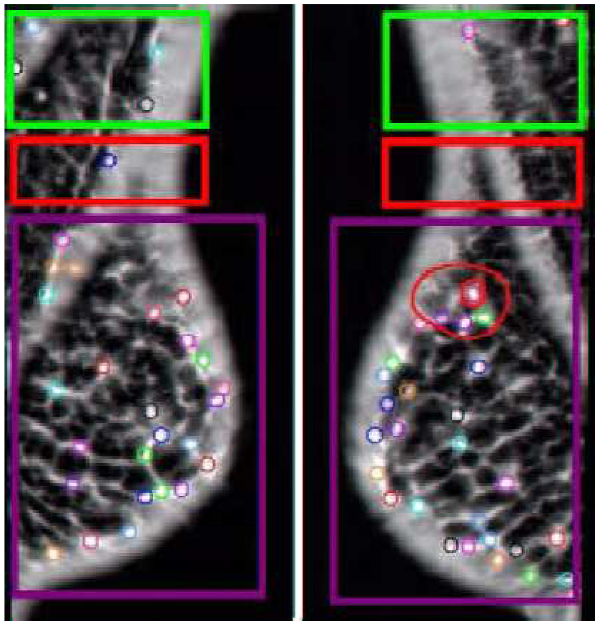
Figure 6.
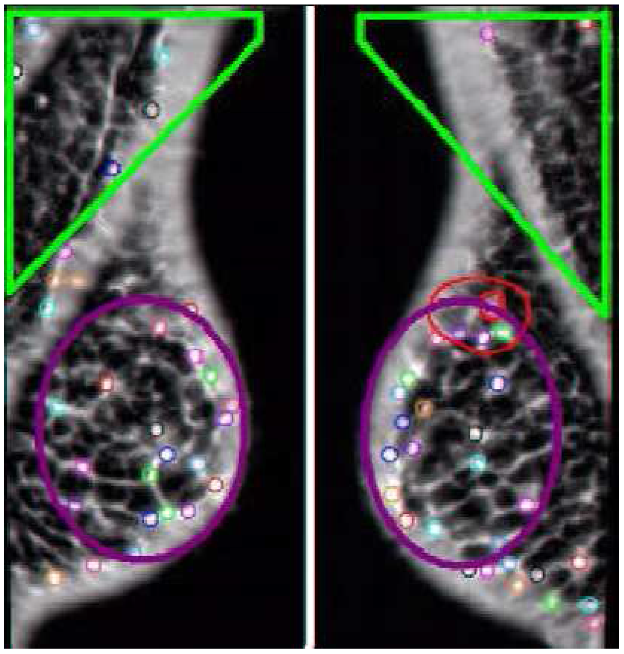
Example Comparison. The AFUM features are the small circles. The automatically created hyper-volumes in this example are the large boxy shapes containing the points, but the same effect can be created with two separators. This case was correctly diagnosed by both the space-based and data-based techniques. Note the red hyper-cluster, which was found to be a significant area in the determination of cancer. In noisy, cancer-free images this area would pick up a statistically equal number of features.
Figure 6.
Example Comparison. The AFUM features are the small circles. The automatically created hyper-volumes in this example are the large boxy shapes containing the points, but the same effect can be created with two separators. This case was correctly diagnosed by both the space-based and data-based techniques. Note the red hyper-cluster, which was found to be a significant area in the determination of cancer. In noisy, cancer-free images this area would pick up a statistically equal number of features.
These alternate definitions of clustering focus on increasing the flexibility of the clustering or on decreasing the required number of parameters. An alternate clustering is shown in Figure 7 where the cluster is designed to avoid a noisy area on the images. The focus on decreasing the number of parameters is required to improve the generalizability of the technique when using supervised learning, which is another adaptation we did to the clustering method.
Figure 7.
The automatically created hyper-volumes in this case are non-space-filling and attempt to avoid a noisy area at the chest wall by not including those features.
Figure 7.
The automatically created hyper-volumes in this case are non-space-filling and attempt to avoid a noisy area at the chest wall by not including those features.

3.2. Supervised Clustering
The second adaptation of the clustering method was the use of supervised learning to maximize the performance on a training set instead of minimizing an objective function. The error function that we minimize is
where
is the normalized weight of that particular case,
and
are the unregistered three-dimensional input features (sorted by one particular feature value for convenience),
is the classification function, P are the parameters of the classification, and cj is the correct classification of the image set j. Note that this technique is being used on image sets, but can be used to compare arbitrary images. The parameters
are learned in order to reduce the error function and includes the parameters of the clustering. Varying the weights of the cancerous and non-cancerous cases allows tuning the performance to achieve fewer false negatives at the expense of higher false positives. The learning was done using exhaustive search in order to guarantee that the result was not caught in a local minimum.
Though the learning was finally done using exhaustive search, we did experiment with hierarchical learning. This is where the first separator is learned, and then the subsequent separators are learned while only changing the parent separator by some fixed percentage and not affecting the grandparent. We also experimented with true hierarchical learning, where the parent is not allowed to vary, but this was found to be ineffective. This has the effect of reducing the number of degrees of freedom to learn by breaking the learning up into multiple levels. The learning of one level is reduced to learning the two child separators and the minimized range of the parent separator, instead of learning the entire set of separators. The inclusion of more separators is self-limiting if the separators are allowed to line up with the parent, thus not breaking up the space and indicating that the hierarchy should end at the parent for that volume of feature space. The application did not require a large number of levels in the hierarchy, allowing the use of exhaustive search to verify the results of the hierarchical learning.
3.3. Image Comparison Distance Functions Using Clusters
The analysis for image comparison that we used performs a comparison of clusters of features in order to maintain both a contextual and spatial comparison while avoiding an exact registration. We experimented with two different models where the clusters are defined using separators and hyper-volumes. We also experimented with a model that compares small clusters of AFUM features between images. The hyper-volume image comparison can be seen in Figure 6, where the points are assigned to clusters that are defined by large volumes of feature space and have a set spatial relationship between each other. The feature-space hyper-volumes have a pre-set registration with the corresponding volumes in the other image. For simplicity, the volumes are assumed to be non-overlapping and space-filling, but this is not required. Additionally, the volumes are assumed to contain the same hyper-volumes in the images of the left and right breasts out of symmetry. This reduces the number of parameters and increases the ability of the model to be generalized to a larger data set, based on the assumption that there are no important anatomical differences between the left and right breasts and that breast cancer is equally as likely to be in the left or right breast. However, when there is a large natural asymmetry to the breasts this assumption may no longer be valid.
In a hyper-volume image comparison, a hyper-volume is assigned all of the suspicious points in the space dA that the hyper-volume spans. The parameters of the hyper-volumes are learned through parametric learning, and any model can be used to characterize the hyper-volumes in feature space. Exact registration of the suspicious points is avoided by using the volumes for the comparisons as they are registered with the corresponding volume in the other image. The feature space is broken up into hyper-volumes as shown in Figure 6. The agglomerated distance D shown in Equation 1 is defined for the comparison of the two point feature sets, and the absolute value of the differences compared against an optimized threshold. Since the features are point features, they are represented using the delta function δ and there is no weighting function yet introduced:
The point sets for the images are represented as {ai} and {bi} for images a and b respectively. The summation over dA is done over all of the clusters which are represented by their hyper-volume dA. The integration is done over the actual hyper-volume dA of the cluster. The summation over i is done over all of the features. The multi-dimensional integral over feature space provides the agglomeration aspect of the distance metric. The hyper-volumes dA provide the agglomeration and are learned along with a threshold in order to optimize the performance of the distance measure at classification. This allows the distance metric to be easily adapted to different image types and imaging techniques, as well as providing a method for incorporating feedback into the distance metric. This distance metric compares the distributions of spatially distributed point sets, and is sensitive to variations in the distribution for image comparison. This is useful for applications such as determining the presence of cancer. There are several other variations to this distance metric that have been explored.
A variation on this distance metric is shown in Equation 2 that learns a threshold for each cluster dA, which has the advantage of being able to emphasize the importance of some areas in the feature space over others. This can be used to distinguish noisy areas where many spurious suspicious points are found from important areas where even small variations are indicative of a lack of similarity. This technique of learning important areas in images can be thought of as an image discovery technique:
A more generalized form of the similarity distance metric is given by equation 3, where the delta function is not the required function and the number of features in each image is not required to be the same. A natural choice for the function g is the probability density function; however, the function g can be determined to try to optimize the retrieval on the particular application:
We tested several variations of the image comparison ideas. The simplest model utilizes only one seperator to create two hyper-volumes and thus only two parameters P = (x1 || y1 || z1, t): one parameter for a separator, one parameter t for a threshold, and Equation 1 for the distance function. This will be called the “two-cluster” analysis. The first parameter x1 || y1 || z1 chooses the best dimension and best position to break up the feature space into volumes and the value in that dimension. The second model used the same parameters and Equation 1, but weighted the learning to give greater weight to the performance on the cancerous cases over the performance on the non-cancerous cases, and this will be called the “two-cluster weighted towards cancer” analysis. The third model used the parameters of the first, but also included an additional parameter that permits selection, so that cases that do not have a minimum number of features in each cluster are not analyzed. This approach used the parameter set P = (x1 || y1 || z1, t, s) where s is a required minimum occupancy of each cluster. This approach is called the “two-cluster with selection” approach. The fourth model used three parameters P = (x1 || y1 || z1, x2 || y2 || z2, t): two parameters for two separators and one for a threshold and is shown in Figure 6. This model will be called “three cluster Equation 1” and Equation 1 is used. The fifth model used three clusters and Equation 2 with the same threshold for each cluster comparison and will be called “three cluster Equation 2.” These models were motivated by the observation that the cancer would change the distribution of the suspicious points, leading to an indication of cancer. An improvement to the method would be to adaptively determine the optimal number of volumes through a split-and-merge type methodology [50].
A different approach explored the importance of the distribution of AFUM feature points, as explored with approaches one through five, versus the clumping of AFUM features together. This sixth approach does not set the number of clusters arbitrarily, but instead learns the number of clusters from the data and learns the best parameterization of the clusters. This image comparisons search for small clumps of AFUM features and then assign a cluster there, as shown in Figure 8, and is called the “small cluster analysis.” The maximum distance between feature points and the minimum features needed to define a cluster are learned on the training set. The clusters were also defined to be centered on a suspicious point because we believed that small clumps of suspicious points tended to form around the central cancer. This assumption may be incorrect, and freeing the cluster centers from that constraint may improve the performance. Exact registration is avoided again by registering the clusters instead of the image or the suspicious points. Comparing the number of clusters in the right image versus the number of clusters in the left image provides a first cut at registering the clusters since a difference in the numbers of clusters implies that some clusters cannot be registered. Improving the cluster registration may improve the performance of the method. This image comparison was motivated by the data, where we observed a small volume of suspicious points at a cancer sites.
Many other approaches were attempted on this dataset. One unsuccessful approach compared the variances of the distribution of suspicious points, while another used a Naive Bayes analysis, and these are compared along with wavelet methods and commercial techniques.
Figure 8.
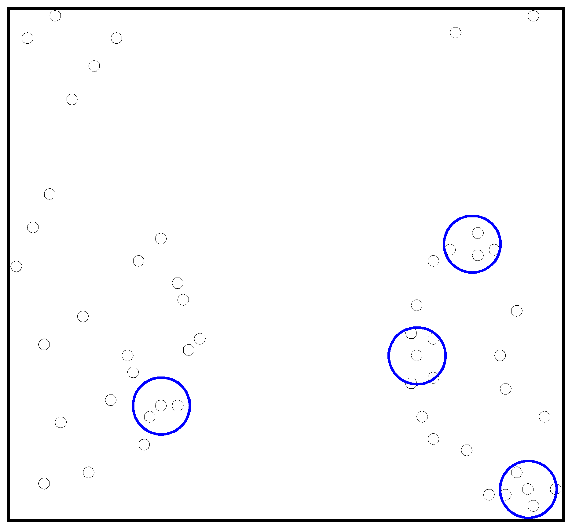
Small Cluster Analysis, a different modeling approach. The AFUM features are the small circles, with the circles on the left coming from the image of the left breast and the circles on the right coming from the image of the right breast. The small clusters are the larger blue circles. This method searches for small clumps of suspicious points and then assigns a cluster there, comparing the number of clusters in the two images, which is a significantly different approach than the one shown in Figure 6 or Figure 7. This method learns the best size for a cluster on the training data. The performance of this approach relative to the other methods showed that AFUM feature clumping was too hindered by the false positive clusters near the breast boundary. This approach may be improved by automatically removing clusters too near the breast boundary.
Figure 8.
Small Cluster Analysis, a different modeling approach. The AFUM features are the small circles, with the circles on the left coming from the image of the left breast and the circles on the right coming from the image of the right breast. The small clusters are the larger blue circles. This method searches for small clumps of suspicious points and then assigns a cluster there, comparing the number of clusters in the two images, which is a significantly different approach than the one shown in Figure 6 or Figure 7. This method learns the best size for a cluster on the training data. The performance of this approach relative to the other methods showed that AFUM feature clumping was too hindered by the false positive clusters near the breast boundary. This approach may be improved by automatically removing clusters too near the breast boundary.

3.4. Evaluation
The image comparisons were applied to the mediolateral oblique (MLO) mammogram views of both the left and right breast of patients that were diagnosed with cancer and patients that were diagnosed as normal, or free from cancer. The analysis was performed over test and training data sets, with cases that were roughly split between normal mammograms and mammograms with malignant spiculated lesions from the Digital Database for Screening Mammography [51]. The focus was on one type of breast cancer which creates spiculated lesions in the breasts. Spiculated lesions are defined as breast cancers with central areas that are usually irregular and with ill-defined borders. Their sizes vary from a few millimeters to several centimeters in diameter and they are very difficult cancers to detect [47].
The training set had 39 non-cancerous cases and 37 cancerous cases, while the test set had 38 non-cancerous cases and 40 cancerous cases. The data is roughly spread across the density of the breasts and the subtlety of the cancer. The breast density and subtlety were specified by an expert radiologist. The subtlety of the cancer shows how difficult it is to determine that there is cancer. The training data set was used to determine optimal parameters the volumes dA. The inputs are the extracted AFUM features for each image in the screening mammogram set, as shown in Figure 3. The output is a classification as either cancerous or non-cancerous. We used exhaustive search because we could, and require only a single stage. These cases indicated that a difference in the clusters of one or more AFUM features indicated cancer in both the two and three cluster experiments.
Figure 9.
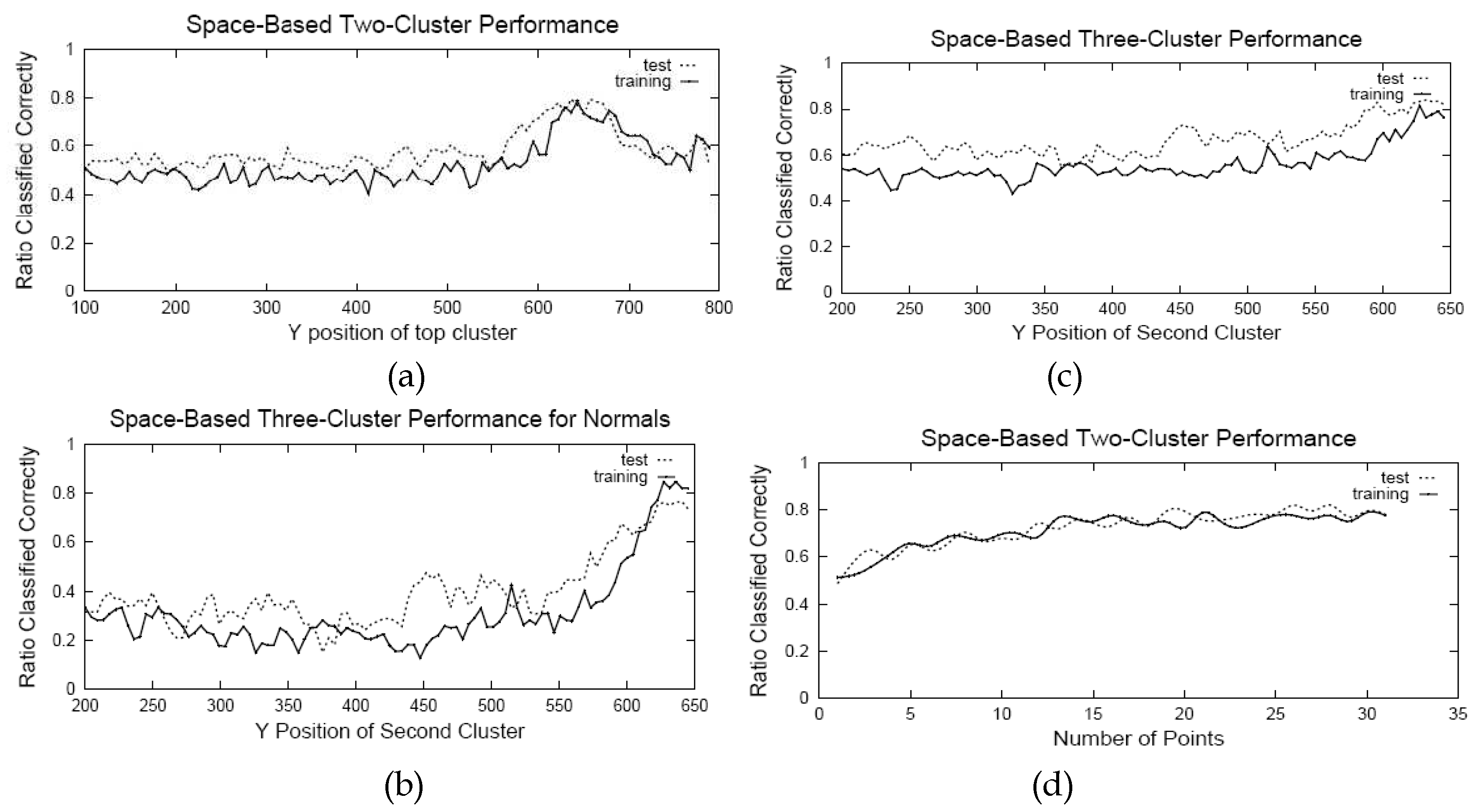
Comparison Data. The maxima in learning the two-cluster method with respect to one of the parameters, the y value parameters P is in (a) and the method is shown to generalize well from training to test data. The same information for the three-cluster method is shown in (b). The performance relative to the number of suspicious points used in the two-cluster technique is in (c). The performance of the three-cluster method on normals, or non-cancerous cases, is shown in (d).
Figure 9.
Comparison Data. The maxima in learning the two-cluster method with respect to one of the parameters, the y value parameters P is in (a) and the method is shown to generalize well from training to test data. The same information for the three-cluster method is shown in (b). The performance relative to the number of suspicious points used in the two-cluster technique is in (c). The performance of the three-cluster method on normals, or non-cancerous cases, is shown in (d).

3.5. Results
Our results are good on all cases of the test set, correctly classifying 80% for the two-cluster as shown in Figure 9a, and 85% of the time for the three-cluster as shown in Figure 9b. The data-defined cluster model results as shown in Figure 9c were not as good, but have the potential for improvement. The results are summarized in Table 1. However, it is much more important to correctly classify the cancerous cases, and by heavily weighting the importance of the cancerous cases, we correctly classified 97% of the cancerous cases with the two-cluster model.
Neither the subtlety nor the density of the cancer had an effect on the results. However, because we have only a limited number of cancerous images, there is some possibility that the imperfect distribution could affect the results of the analysis.
The comparison with a commercial system shows that the results are surprisingly good. Our method showed an improvement of 26% on the non-cancerous cases while matching the performance on cancerous cases with the R2 ImageChecker system [29]. The inclusion of additional factors other than asymmetry in the method should improve the results. However, the data sets used are different, as the R2 ImageChecker data contains all cancer types and our method has only the difficult to detect spiculated lesions. The R2 ImageChecker data set also had a much higher proportion of non-cancerous mammograms to cancerous cases. Our performance is shown in Figure 10.
One of the parameters that was learned was the optimal number of AFUM features to use in the analysis, and the results were always at or near the top of the range that we used, varying from 29 to 32 features depending on the model and weightings as shown in Figure 9d. This was surprising because the cancer was usually in the top sixteen if not the top eight points. However, the suspicious points do tend to cluster around a cancer, so including more suspicious points may create a greater distortion of the underlying distribution than fewer points. The learning algorithm does not get the number of points directly, only the cluster differences, so the inclusion of more points should not skew this analysis.
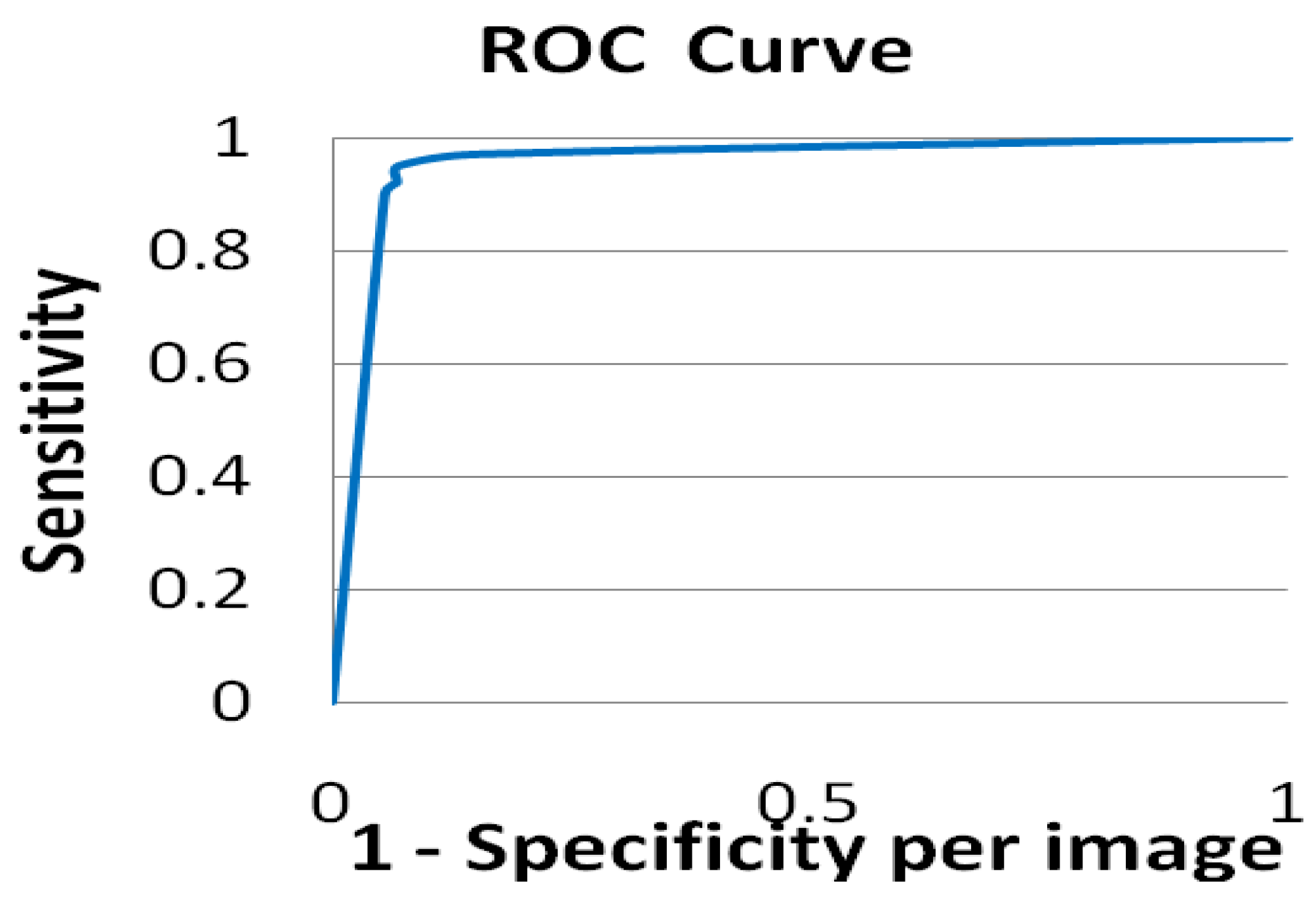
Figure 10.
ROC curve demonstrating the effectiveness of this distance metric at diagnosing mammograms.
Figure 10.
ROC curve demonstrating the effectiveness of this distance metric at diagnosing mammograms.

| Method | Cancerous | Non-Cancerous |
|---|---|---|
| Three-Cluster Equation 1 | 90% | 79% |
| Two-Cluster Weighted Toward Cancer Equation 1 | 97% | 42% |
| Two Cluster Equation 1 | 87% | 71% |
| R2 Image Checker* [29] | 96% | 33% |
| Wavelet* [27] | 77% | 77% |
| Naïve Bayes | 51% | 49% |
| Three-Cluster Equation 2 | 95% | 73% |
| Variance Analysis | 60% | 60% |
| Two-Cluster With Selection Equation 1 | 92% | 73% |
| Small-Cluster Analysis | 51% | 56% |
An interesting result from the three-cluster analysis showed that these methods could discover areas in images that are important for the classification, and this is demonstrated in Figure 9b,c. The analysis found a region of interest for diagnosing a mammogram as non-cancerous. These techniques can be used as a method for probing feature space for important areas.
Our methods make use of a spatial analysis of the suspicious points, and its success is an encouraging sign for the investigation and utilization of more complicated non-local analysis techniques in medical imaging and analysis.
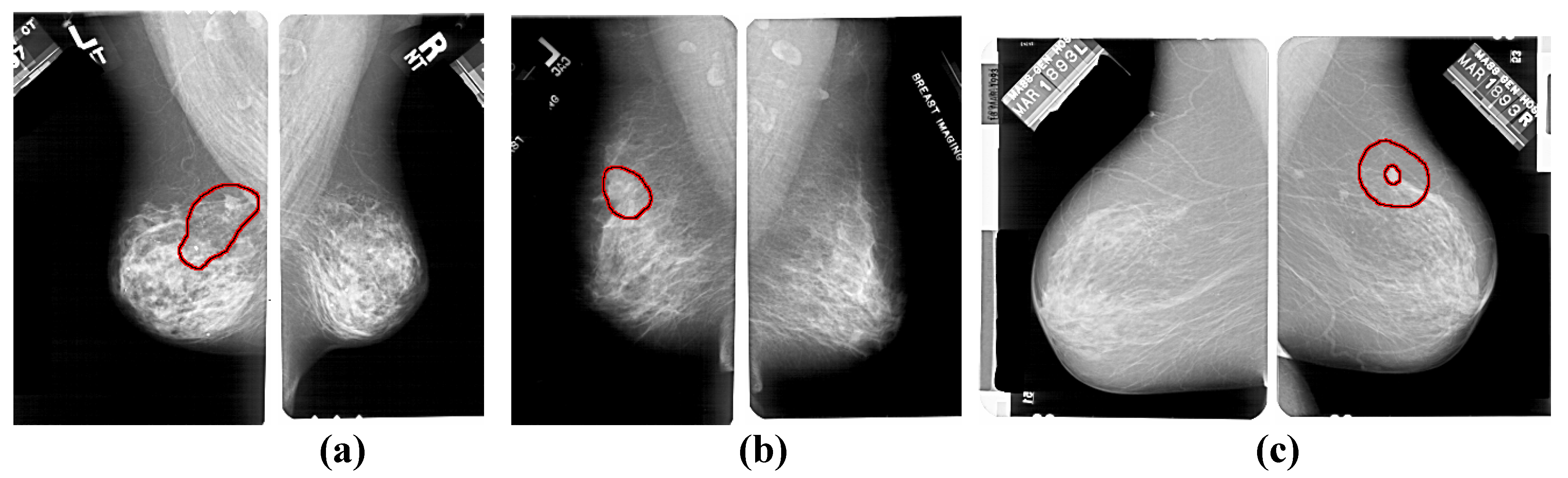
Analysis of the misdiagnosed cases in Figure 11 demonstrates a potential flaw in the method. When there is too much structure in one area that draws the relatively simple features that we are using into it on just a small number of cases, the method can misclassify them. A potential improvement is to incorporate a second level of classifiers that would analyze the missed diagnoses.
Figure 11.
The left and right MLO views of three cases that were misdiagnosed by the three cluster approach. The cancerous areas are outlined in red. There are significant variations in the size and morphology of spiculated lesions. Note that cases (b) and (c) both have significant natural asymmetry of the breasts from left to right.

4. Improvement to CAD
Having developed the distance function for medical images described in Section 3, we used the results to help improve the computer-aided detection of breast cancer. Computer-aided detection (CAD) of mammograms could be used to avoid missed diagnoses, and has been shown to increase the number of cancers detected by more than nineteen percent [4]. Improving the effectiveness of CAD could improve the detection of breast cancer, and could improve the survival rate by detecting the cancer earlier.
The typical CAD system takes in a mammogram set and displays it for the radiologist. The system also provides markers on potential cancerous sites as found by the system. The determination of these markers and the evaluation of their effectiveness in helping radiologists are the main thrust of CAD research. The hope for CAD is that the cancers missed by the radiologist are marked by the computer and brought to the attention of the radiologist.
Most computer-aided detection (CAD) systems are tested on images which contain cancer on the assumption that images without cancer would produce the same number of false positives. However, a pre-screening system is designed to remove the normal cases from consideration, and so the inclusion of a pre-screening system into CAD dramatically reduces the number of false positives reported by the CAD system. We define three methods for the inclusion of pre-screening into CAD.
4.1. Incorporation into CAD
There are three basic methods for including pre-screening into CAD analysis. The first is the strict method, where the pre-screening removes the non-cancerous cases entirely from the consideration of the CAD software. The second is the probabilistic method, where the probability of the case being cancerous or non-cancerous is determined by the pre-screening system and then incorporated into the CAD analysis. The third is an optimal method, which uses learning to try to determine the optimal factors for the inclusion of the pre-screening results into the CAD analysis. These methods will be defined and compared below.
The strict method is the simplest to define. Images that are screened as normal are removed from consideration by the CAD analysis. Since there are no false positives drawn from these cases, the number of false positives per image decreases. This is the most effective technique at reducing the number of false positives, but it is also the most dangerous as mistakes by the pre-screening system cannot be rectified by the CAD system.
The probabilistic method relies on the statistics of the pre-screening method to adjust the output of the CAD system. To incorporate pre-screening into a CAD system, we made use of Bayes Theorem, P(CancerSite | Pre-screen) = {P(Pre-screen | CancerSite) P(CancerSite) / P(Pre-screen)}. The sites where pre-screening indicates cancer are thus given an increased probability of being cancerous, while sites where pre-screening does not indicate cancer are given a reduced probability of being cancerous. Since the pre-screening measurement is applied to an entire case, all of the sites in those cases are affected similarly.
The optimal approach is a variant of the probabilistic approach, but instead of deriving the change from the underlying probabilities, the change is learned on a training set of cases. In theory, this approach can optimize the incorporation of pre-screening into CAD, but can be difficult in practice. In this case, P(CancerSite | Pre-screen) = A(Pre-screen) P(CancerSite), where A(Pre-screen) is the learned adjustment factor. This approach has more flexibility than the probabilistic approach, but is much harder to implement. The choice of what to optimize is also a concern. There are two main options, optimizing the area under the ROC curve or optimizing the accuracy of the CAD results in a certain range of specificity. Both approaches were attempted and will be discussed.
4.2. Results of Incorporation into CAD
The analysis was performed with the same cases that were used for the analysis in Section 3. The training data set was used to determine the parameter A(Pre-screen) for the optimal approach. The other approaches were tested against the same test set in order to be unbiased. An AFUM-based CAD system [44] was used as the CAD basis.
The results were good at low numbers of false positives in all three techniques, and it is at high and medium numbers of false positives where techniques distinguish themselves. Using the probabilistic approach to incorporate pre-screening into CAD is shown to work well at low numbers of false positives per image and can improve the performance by over 70%, but at high levels of false positives per image, this technique has minimal effect. This is expected since using Bayes Theorem merely reduces the probability of the false positives and does not eliminate them.
The results of the strict approach are identical to the results of the probabilistic approach at low levels of false positives, but diverge at higher levels of false positives. Since this approach eliminates the false positives instead of just diminishing them, the results at high levels of false positives per image are worse than the probabilistic approach because true positives are eliminated. However, in medium levels of false positives, the performance is significantly better than the probabilistic approach.
The optimal approach was tuned to determine the best performance at both low levels of false positives and the overall area under the ROC curve. The performance under both converged to the strict approach; however, this may be due to the pre-screening technique that was chosen.
The overall performance is still strongly dependent on the effectiveness of the CAD system. The accuracy of the pre-screening is essential in order to prevent true positives from having their probabilities diminished, and the specificity is important for improving the effectiveness of the CAD system.
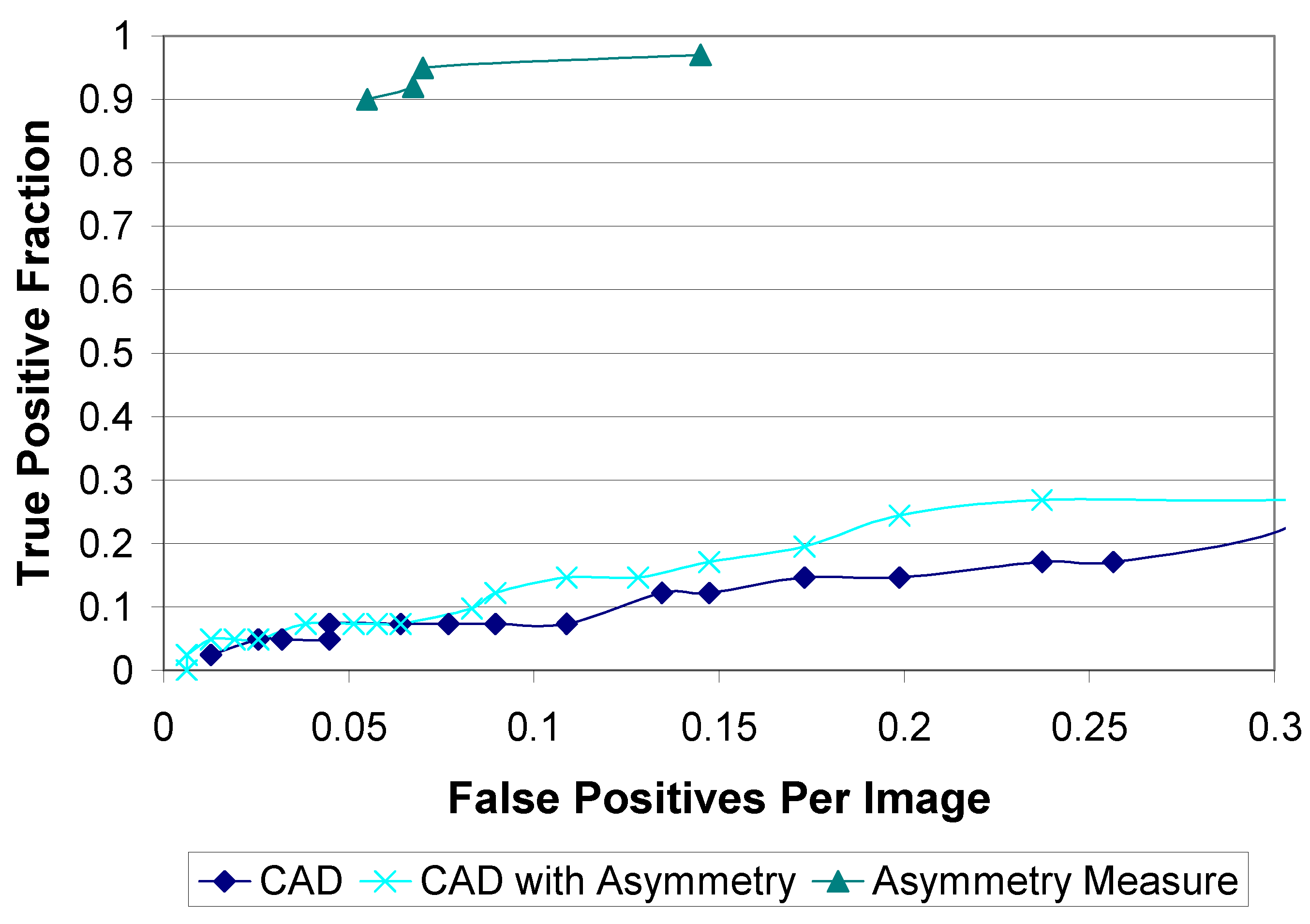
The incorporation of the classification results back into the original CAD system does significantly improve the original CAD system, as shown in Figure 12. The results of incorporating our classification into CAD were good, increasing the accuracy by up to 71% at a set level of false positives per image. The improvement is most apparent at low levels of false positives. Incorporating asymmetry into CAD can improve the effectiveness at low levels of false positives per image. We incorporated it as an afterthought, while it would be more effective as a feature used at the beginning of the CAD prompt calculation process. However, we did determine that asymmetry is a powerful technique by itself or incorporated into CAD. This indicates that further research into techniques that can compare images and thus measure asymmetry in mammograms may significantly improve the effectiveness of CAD algorithms.
Figure 12.
ROC curve comparing the CAD system before and after the inclusion of the Three-Cluster approach to measuring asymmetry. The inclusion of asymmetry improves the CAD system by up to 77%. The asymmetry measure has a very low level of false positives per image because it does not try to determine the position of the cancer; it merely determines the presence of cancer. This CAD is done on the same images as mentioned in Section 3.4.

5. Conclusions
This work touched on many of the problems facing the classification and retrieval of cancer images and data. We developed a method for differencing and classifying images, which we then incorporated into CAD. Our results are strong on all cases of the test set for classifying breast cancer images, correctly classifying with 85% accuracy and our technique outperforms both the best academic and commercial approaches, suggesting that this is an important technique in the classification of mammograms. We have also shown that using the image comparisons to determine the classification is insensitive to the parameters of the approach.
We created and compared multiple models, demonstrating improved results over both academic and commercial approaches. We also defined a new distance measure for the comparison of point sets and demonstrate its effectiveness in this application. The coupling of this distance measure with the parametric learning of clusters led to a highly effective classification technique.
The clusters also discovered an area of interest in mammogram comparisons which improved the diagnosis of mammograms that did not have cancer. More clusters might improve the technique, or, more importantly, they might lead to the discovery of more areas of interest. The separation of the clusters from direct classification allowed a greater exploration of the feature space by the algorithm. We suggested several ways that might improve on the methods that we used to compare mammograms.
The incorporation of the classification results back into the original CAD system does significantly improve the original CAD system. The results of incorporating our classification into CAD were good, increasing the accuracy by up to 71% at a set level of false positives per image. The improvement is most apparent at low levels of false positives. Incorporating asymmetry into CAD can improve the effectiveness at low levels of false positives per image. We also determined that asymmetry is a powerful technique by itself or incorporated into CAD. This indicates that further research into techniques that can compare images and thus measure asymmetry in mammograms may significantly improve the effectiveness of CAD algorithms.
References
- American Cancer Society. Breast Cancer Facts and Figures 1999–2000; American Cancer Society: Atlanta, GA, USA, 1999. [Google Scholar]
- Linda, J.; Burhenne, W.; Wood, S.A.; D’Orsi, C.J.; Feig, S.A.; Kopans, D.B.; O’Shaughnessy, K.F.; Sickles, E.A.; Tabar, L.; Vyborny, C.J.; Castellino, R.A. Potential contribution of computer-aided detection to the sensitivity of screening mammography. Radiology 2000, 215, 554–562. [Google Scholar]
- Freer, T.W.; Ulissey, M.J. Screening mammography with computer-aided detection: Prospective study of 12,860 patients in a community breast center. Radiology 2001, 220, 781–786. [Google Scholar] [CrossRef] [PubMed]
- Gur, D.; Sumkin, J.H.; Rockette, H.E.; Ganott, M.; Hakim, C.; Hardesty, L.; Poller, W.R.; Shah, R.; Wallace, L. Changes in breast cancer detection and mammography recall rates after the introduction of a computer-aided detection system. J. Natl. Cancer Inst. 2004, 96, 185–190. [Google Scholar] [CrossRef] [PubMed]
- Khoo, L.A.; Taylor, P.; Given-Wilson, R.M. Computer-aided detection in the United Kingdom national breast screening programme: prospective study. Radiology 2005, 237, 444–449. [Google Scholar] [CrossRef] [PubMed]
- Ko, J.M.; Nicholas, M.J.; Mendel, J.B.; Slanetz, P.J. Prospective assessment of computer-aided detection in interpretation of screening mammograms. Am. J. Roentgenol. 2006, 187, 1483–1491. [Google Scholar] [CrossRef] [PubMed]
- Gur, D.; Stalder, J.S.; Hardesty, L.A.; Zheng, B.; Sumkin, J.H.; Chough, D.M.; Shindel, B.E.; Rockette, H.E. Computer-aided detection performance in mammographic examination of masses: assessment. Radiology 2004, 233, 418–423. [Google Scholar] [CrossRef] [PubMed]
- Zheng, B.; Leader, J.K.; Abrams, G.S.; Lu, A.H.; Wallace, L.P.; Maitz, G.S.; Gur, D. Multiviewbased computer-aided detection scheme for breast masses. Med. Phys. 2006, 33, 3135–3143. [Google Scholar] [CrossRef] [PubMed]
- Nishikawa, R.M.; Kallergi, M. Computer-aided detection in its present form is not an effective aid for screening mammography. Med. Phys. 2006, 33, 811–814. [Google Scholar] [CrossRef] [PubMed]
- Fenton, J.J.; Taplin, S.H.; Carney, P.A.; Abraham, L.; Sickles, E.A.; D’Orsi, C.; Berns, E.A.; Cutter, G.; Hendrick, R.E.; Barlow, W.E.; Elmore, J.G. Influence of computer-aided detection on performance of screening mammography. New England J. Med. 2007, 356, 1399–1409. [Google Scholar] [CrossRef] [PubMed]
- Tourassi, G.D.; Vargas-Voracek, R.; Catarious, D.M.; Floyd, C.E. Computer-assisted detection of mammographic masses: a template matching scheme based on mutual information. Med. Phys. 2003, 30, 2123–2130. [Google Scholar] [CrossRef] [PubMed]
- Tahmoush, D.; Samet, H. Image similarity and asymmetry to improve computer-aided detection of breast cancer. In Digital Mammography; Astley, S.M., Brady, M., Rose, C., Zwiggelaar, R., Eds.; Springer: Manchester, UK, 2006; pp. 221–228. [Google Scholar]
- El-Napa, I.; Yang, Y.; Galatsanos, N.P.; Nishikawa, R.M.; Wernick, M.N. A similarity learning approach to content-based image retrieval: application to digital mammography. IEEE Trans. Med. Imaging 2004, 23, 1233–1244. [Google Scholar] [CrossRef] [PubMed]
- Wei, C.; Li, C.; Wilson, R. A general framework for content-based medical image retrieval with its application to mammograms. Proc. SPIE 2005, 5748, 134–143. [Google Scholar]
- Alto, H.; Rangayyan, R.M.; Desautels, J.E. Content-based retrieval and analysis of mammographic masses. J. Electron. Imaging 2005, 14, 023016. [Google Scholar] [CrossRef]
- Tao, Y.; Lo, S.B.; Freedman, M.T.; Xuan, J. A preliminary study of content-based mammographic masses retrieval. Proc. SPIE 2007, 6514, 65141Z. [Google Scholar]
- Kinoshita, S.K.; de Azevedo-Marques, P.M.; Pereira, R.R.; Rodrigues, J.; Rangayyan, R. Content-based retrieval of mammograms using visual features related to breast density patterns. J. Digit. Imaging 2007, 20, 172–190. [Google Scholar] [CrossRef] [PubMed]
- Zheng, B.; Mello-Thoms, C.; Wang, X.; Abrams, G.S.; Sumkin, J.H.; Chough, D.M.; Ganott, M.A.; Lu, A.; Gur, D. Interactive computer aided diagnosis of breast masses: computerized selection of visually similar image sets from a reference library. Acad. Radiol. 2007, 14, 917–927. [Google Scholar]
- Mazurowski, M.A.; Habas, P.A.; Zurada, J.M.; Tourassi, G.D. Decision optimization of case-based computer-aided decision systems using genetic algorithm with application to mammography. Phys. Med. Biol. 2008, 53, 895–908. [Google Scholar] [CrossRef] [PubMed]
- Rosa, N.A.; Felipe, J.C.; Traina, A.J.; Rangayyan, R.M.; Azevedo-Marques, P.M. Using relevance feedback to reduce the semantic gap in content-based image retrieval of mammographic masses. In Proceedings of the 30th Annual International Conference of the IEEE Engineering in Medicine and Biology Society, Vancouver, BC, USA, August 20–25, 2008; pp. 406–409.
- Park, S.C.; Pu, J.; Zheng, B. Improving performance of computer-aided detection scheme by combining results from two machine learning classifiers. Acad. Radiol. 2009, 16, 266–274. [Google Scholar] [CrossRef] [PubMed]
- Giger, M.L.; Huo, Z.; Vyborny, C.J.; Lan, L.; Bonta, I.R.; Horsch, K.; Nishikawa, R.M.; Rosenbourgh, I. Intelligent CAD workstation for breast imaging using similarity to known lesions and multiple visual prompt aides. Proc. SPIE 2002, 4684, 768–773. [Google Scholar]
- Tahmoush, D.; Samet, H. Image differencing approaches to medical image classification. In Proceedings of the 36th Applied Imagery Pattern Recognition Workshop, Washington, DC, USA, 2007; pp. 22–27.
- Tahmoush, D.; Samet, H. An improved asymmetry measure to detect breast cancer. Proc. SPIE 2007, 6514, 65141Q. [Google Scholar]
- Tahmoush, D.; Samet, H. Using image similarity and asymmetry to detect breast cancer. Proc. SPIE 2006, 6144, 61441S. [Google Scholar]
- Tahmoush, D. Augmenting medical image diagnosis through image similarity. Proc. SPIE 2009, 7260, 7260–7280. [Google Scholar]
- Ferrari, R.J.; Rangayyan, R.M.; Desautels, J.E.L.; Frere, A.F. Analysis of asymmetry in mammograms via directional filtering with Gabor wavelets. IEEE Trans. Med. Imaging 2001, 20, 953–964. [Google Scholar] [CrossRef] [PubMed]
- Astley, S.; Mistry, T.; Boggis, C.R.M.; Hillier, V.F. Should we use humans or a machine to pre-screen mammograms? In Proceedings of the Sixth International Workshop on Digital Mammography, Bremen, Germany, June 22-25, 2002; pp. 476–480.
- Astley, S.; Gilbert, F.J. Computer-aided detection in mammography. Clin. Radiol. 2004, 59, 390–399. [Google Scholar] [CrossRef] [PubMed]
- Faloutsos, C.; Barber, R.; Flickner, M.; Hafner, J.; Niblack, W.; Petkovic, D.; Equitz, W. Efficient and effective querying by image content. J. Intell. Inf. Syst. 1994, 3, 231–262. [Google Scholar] [CrossRef]
- Goldberger, J.; Gordon, S.; Greenspan, H. An efficient image similarity measure based on approximations of kl-divergence between two gaussian mixtures. In Proceedings of the Ninth IEEE International Conference on Computer Vision, Nice, France, October 13–16, 2003; Vol. 1, pp. 487–493.
- Gudivada, V.; Raghavan, V. Design and evaluation of algorithms for image retrieval by spatial similarity. ACM Trans. Inf. Syst. 1995, 13, 115–144. [Google Scholar] [CrossRef]
- Soffer, A.; Samet, H. Pictorial queries by image similarity. In Proceedings of the 13th International Conference on Pattern Recognition, Vienna, Austria, 1996; Vol. 3, pp. 114–119.
- Swett, H.A.; Miller, P.L. Icon: a computer-based approach to differential diagnosis in radiology. Radiology 1987, 163, 555–558. [Google Scholar] [CrossRef] [PubMed]
- Guimond, A.; Subsol, G. Automatic MRI database exploration and applications. Pattern Recognition Artif. Intell. 1997, 11, 1345–1365. [Google Scholar] [CrossRef]
- Gondra, I.; Heisterkamp, D.R. Learning in region-based image retrieval with generalized support vector machines. In Proceedings of the Computer Vision and Pattern Recognition, Washington, DC, USA, June 27–July 2, 2004; p. 149.
- Miller, P.; Astley, S. Detection of breast asymmetry using anatomical features. In Proceedings of the International Society for Optical Engineering Conference on Biomedical Image Processing and Biomedical Visualization, San Jose, CA, USA, January 31–Feburary 5, 1993; Vol. 1905, pp. 433–442.
- Wirth, M.A.; Choi, C.; Jennings, A. A nonrigid-body approach to matching mammograms. In Proceedings of the 7th International Conference on Image Processing and its Applications, San Jose, CA, USA, July 26–27, 1999; Vol. 2, pp. 484–488.
- Yin, F.F.; Giger, M.L.; Doi, K.; Metz, C.E.; Vyborny, C.J.; Schmidt, R.A. Computerized detection of masses in digital mammograms: analysis of bilateral subtraction images. Med. Phys. 1991, 18, 955–963. [Google Scholar] [CrossRef] [PubMed]
- Vujovic, N.; Brzakovic, D. Establishing the correspondence between control points in pairs of Mammographic images. IEEE Trans. Image Process. 1997, 6, 1388–1399. [Google Scholar] [CrossRef] [PubMed]
- Sallam, M.; Bowyer, K.W. Registering time-sequences of mammograms using a two-dimensional unwarping technique. In Digital Mammography; Elsevier: Amsterdam, The Netherlands, 1996; pp. 291–296. [Google Scholar]
- Yao, J.; Taylor, R. Assessing accuracy factors in deformable 2D/3D medical image registration using a statistical pelvis model. In Proceedings of the Ninth IEEE International Conference on Computer Vision, Nice, France, October 13–16, 2003; Vol. 2, pp. 1329–1334.
- Wirth, M.A.; Narhan, J.; Gray, D. Nonrigid mammogram registration using mutual information. Proc. SPIE 2002, 4684, 562–573. [Google Scholar]
- Heath, M.D.; Bowyer, K.W. Mass detection by relative image intensity. In Digital Mammography; Medical Physics Publishing: Madison, WI, USA, 2000; pp. 219–255. [Google Scholar]
- Rahbar, G.; Sie, A.C.; Hansen, G.C.; Prince, J.S.; Melany, M.L.; Reynolds, H.E.; Jackson, V.P.; Sayre, J.W.; Bassett, L.W. Benign versus malignant solid breast masses: US differentiation. Radiology 1999, 213, 889–894. [Google Scholar] [CrossRef] [PubMed]
- Kalman, B.L.; Kwasny, S.C.; Reinus, W.R. Diagnostic screening of digital mammograms using wavelets and neural networks to extract structure; Technical Report No. 98-20; Washington University: Washington, DC, USA, 1998. [Google Scholar]
- Lui, S.; Babbs, C.F.; Delp, E.J. Multiresolution detection of spiculated lesions in digital mammograms. IEEE Trans. Image Process. 2001, 6, 874–884. [Google Scholar]
- Campanini, R.; Bazzani, A.; Bevilacqua, A.; Bollini, D. A novel approach to mass detection in digital mammography based on support vector machines. In Proceedings of the 6th International Workshop on Digital Mammography, Bremen, Germany, June 22–25, 2002; pp. 399–401.
- Dettling, M.; Buhlmann, P. Boosting for tumor classification with gene expression data. Bioinformatics 2003, 19, 1061–1069. [Google Scholar] [CrossRef] [PubMed]
- Horowitz, S.L.; Pavlidis, T. Picture segmentation by a tree traversal algorithm. JACM 1976, 23, 368–388. [Google Scholar] [CrossRef]
- Heath, M.D.; Bowyer, K.W.; Kopans, D.; Kegelmeyer, P., Jr.; Moore, R.; Chang, K.; Munishkumaran, S. Current status of the digital database for screening mammography. In Digital Mammography; Kluwer Academic Publishers: Boston, MA, USA, 1998; pp. 457–460. [Google Scholar]
© 2009 by the authors; licensee Molecular Diversity Preservation International, Basel, Switzerland. This article is an open-access article distributed under the terms and conditions of the Creative Commons Attribution license ( http://creativecommons.org/licenses/by/3.0/).
Share and Cite
MDPI and ACS Style
Tahmoush, D. Image Similarity to Improve the Classification of Breast Cancer Images. Algorithms 2009, 2, 1503-1525. https://doi.org/10.3390/a2041503
AMA Style
Tahmoush D. Image Similarity to Improve the Classification of Breast Cancer Images. Algorithms. 2009; 2(4):1503-1525. https://doi.org/10.3390/a2041503
Chicago/Turabian StyleTahmoush, Dave. 2009. "Image Similarity to Improve the Classification of Breast Cancer Images" Algorithms 2, no. 4: 1503-1525. https://doi.org/10.3390/a2041503