A Clinical Decision Support Framework for Incremental Polyps Classification in Virtual Colonoscopy

Abstract

We present in this paper a novel dynamic learning method for classifying polyp candidate detections in Computed Tomographic Colonography (CTC) using an adaptation of the Least Square Support Vector Machine (LS-SVM). The proposed technique, called Weighted Proximal Support Vector Machines (WP-SVM), extends the offline capabilities of the SVM scheme to address practical CTC applications. Incremental data are incorporated in the WP-SVM as a weighted vector space, and the only storage requirements are the hyper-plane parameters. WP-SVM performance evaluation based on 169 clinical CTC cases using a 3D computer-aided diagnosis (CAD) scheme for feature reduction comparable favorably with previously published CTC CAD studies that have however involved only binary and offline classification schemes. The experimental results obtained from iteratively applying WP-SVM to improve detection sensitivity demonstrate its viability for incremental learning, thereby motivating further follow on research to address a wider range of true positive subclasses such as pedunculated, sessile, and flat polyps, and over a wider range of false positive subclasses such as folds, stool, and tagged materials.

1. Introduction

Due to the recent advancements in Computed Tomography (CT) technology, and with more than 57,000 colon cancer deaths per year in the United States, CT Colonography (CTC), also known as virtual colonoscopy, is becoming a promising tool for early diagnosis of colon cancer. CTC is a minimally invasive technique that detects colorectal polyps and masses based on the CT scans of distended colon [1]. One of the major obstacles for CTC to be an effective tool for detecting polyps is that radiologists’ expertise is required for analyzing the CTC images, in particular, for the detection of small polyps. Because diagnosis interpretation is a complicated task and any erroneous decision may lead to painful consequences for patients, computer-aided detection (CAD) of polyps would provide clinical decision support systems that benefit patients from correct clinical decisions by reducing the variability of the detection accuracy among radiologists [1]. Such a CAD system typically employs a shape-based method for the initial detection of polyp candidates, followed by a machine learning (ML) method for the classification of polyps from non-polyps (normal colonic structures). The CAD system then generates the final list of polyps that are provided to the radiologist as a “second opinion” [2]. Typically, the input to a CAD system is a large number of CT images, ranging from 300 to 3000 images per patient.

The large amount of data is one of the major obstacles for the ML method in any CAD system to be trained. Moreover, to update the CAD system, the ML method needs to be retrained when new CTC patient image data become available. Therefore, the need to scale up inductive learning algorithms in CAD systems is drastically increasing in order to extract valid and novel patterns from incremental data without a major ML retrain. Dynamic, incremental, or online learning refers, in this context, to the situation where a training image data set is not fully available at the beginning of the learning process. The data can arrive at different time intervals and need to be incorporated into the training data to preserve the class concept. Thus, constructing a ML method capable of incremental classification as opposed to batch-mode learning is very attractive and will become a strategic necessity for CTC because of a few reasons. First, the training period is the most significant resource-intensive element in ML. Second, the CTC data has a continuous, large and unbalanced stream by nature which makes it an ideal candidate for online learning.

To the best of our knowledge, no prior work has addressed incremental multi-classification of polyps using a support vector machine (SVM) approach within the framework of dynamic learning. The novel method we present in this work is called Weighted Proximal Support Vector Machine (WP-SVM) and extends traditional SVM beyond its existing static learning context to handle dynamic and multiple classifications of unbalanced data sets of polyps. The selection of SVM as a machine learning tool for assisting in CTC clinical decisions stems from several of its main advantages: SVM has its roots in statistical learning theory which ensures strong learning and generalization capabilities. It is computationally efficient in learning a hyper-plane that correctly classifies the high dimensional feature space and it is also highly resistant to noisy data [3].

The remainder of this paper is organized as follows: Section 2 presents an overview of multi-classification Least Square SVM (LS-SVM) principles. Section 3 covers our proposed multi-classification WP-SVM techniques for unbalanced data sets. Section 4 validates the effectiveness of WP-SVM in terms of detection performance, computation time, and storage requirements. Finally, Section 5 concludes this work with remarks and outlines for future research.

2. Multi-Classification LS-SVM Survey

SVM technique as invented by Boser, Guyon and Vapnik was first introduced during the Computational Learning Theory (COLT) conference of 1992 [4] and since then it has established itself as one of the leading approaches in the pattern recognition and the machine learning areas, as demonstrated by the results obtained by a broad range of practical applications and recent research work [5,6,7,8,9,10,11,12,13,14,15,16,17,18,19,20,21,22,23,24,25,26,27]. In terms of structural or representational capacity, SVM behaves like a neural network, but it differs in the learning technique.SVM solves a quadratic programming (QP) problem and finds a computationally efficient way of learning a hyper-plane that correctly classifies the high-dimensional feature space after using a linear combination of kernel functions that have to be positive definite [28]. With kernel functions centered on the training input data, SVM minimizes the confidence interval and keeps the training error e fixed while retaining only the support vectors (SV) from the input data.

For instance, given a classical linearly separable multi-classification task with attributes or feature sets <f₁,f₂,...f_f> defined as ${\left\{x_i,y_i\right\}}_{i=1}^N$, where $x_i\in R^f$ represents the i^th input image and y_i the output class, an LS-SVM as introduced in [8] optimizes the objective function

$$\mathrm{Objective\; function:}\frac{1}{2}{\displaystyle \sum _{m=1}^c{w}_m^T\cdot w_m}+\frac{\lambda }{c}{{\displaystyle \sum _{i=1}^N{\displaystyle \sum _{m\ne y_i}^c(e_i^m)}}}^2$$

(1)

where λ is a suitable positive penalty parameter that controls the tradeoff between the classification error e of the c different classes and the margin maximization during the training phase. The error term e, often referred to as the slack variable, accounts for the non-separable data points. Hsu and Lin [29] showed that SVM accuracy rates in general are influenced by the selection of λ which varies depending on the problem under investigation. The selection of λ can be found heuristically or by a grid search.

Depending on the decomposing strategy for converting the multi-classification problem into a set of binary ones, the ML constraint can be formulated as a multi-classification objective function, one-versus-rest, pair-wise, or error-correcting output code [9]. The multi-classification objective function has probably the most compact form as it optimizes the problem into a one single step. It constructs c two-class rules, where each classifier separates training vectors of class y_i from the other m classes using the constraint of the hyper-planes defined by their slopes w and intercepts b:

$$\mathrm{Constraint}:w_{y_i}^T{x}_i+b_{y_i}\ge w_m^T{x}_i+b_m-2-e_i^m$$

(2)

LS-SVM classifiers reduce the optimization problem from a QP to a linear one and optimize the Lagrangian as:

$$L_p(w,b,e,\alpha )=\frac{1}{2}{w}^{T}w+\frac{\lambda }{c}{{\displaystyle \sum _{i=1}^N{\displaystyle \sum _{m\ne y_i}^c(e_i^m)}}}^2-{\displaystyle \sum _{i=1}^N{\alpha }_i{\displaystyle \sum _{m\ne y_i}^c((w_{y_i}-w_m)x_i+(b_{y_i}-b_m)-2}}+e_i)$$

(3)

where α_i represent the Lagrange multipliers which can be either positive or negative. These parameters are derived from the Karush Kuhn-Tucker (KKT) conditions that are valid as long as the objective function and conditions stay convex [28]. The LS-SVM solution can be re-written as a linear system of equations in a matrix format as:

$$\left[\begin{array}{cc}0& Y^T\\ Y& Z{Z}^T+\raisebox{1ex}{${\lambda }^{-1}I$}\!\left/ \!\raisebox{-1ex}{$c$}\right.\end{array}\right]\left[\begin{array}{c}b\\ \alpha \end{array}\right]=\left[\begin{array}{c}0\\ I\end{array}\right]$$

(4)

where $Z=(x_1^T{y}_1;\dots ;x_N^T{y}_N)$, $Y=[y_1;\dots ;y_N]$, $I=[1;\dots 1]$, and $\alpha =[{\alpha }_1;\dots ;{\alpha }_N]$

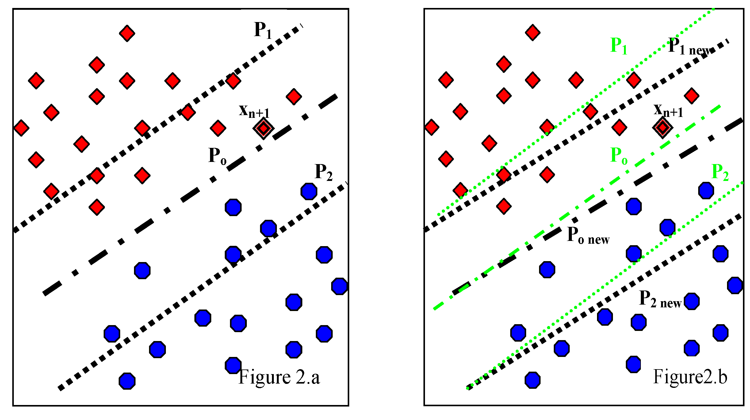
3. Proposed multi-classification WP-SVM

3.1. Proposed Multi-Classification

We propose several novel modifications to the standard multi-classification LS-SVM as highlighted in Section 2. First, we modify the objective function represented by Eq. (1) by adding the plane intercept b in order to uniquely define the hyper-plane by its slope and intercept. Second, because the input data can be unbalanced with respect to the class distribution, and because the penalty parameter of Eq. (1) could be biased towards controlling the overall error term e at the expense of specific classes, we include a new controlling parameter ζ which acts as a local penalty variable for each class. The proposed new objective function is

$$\frac{1}{2}{\displaystyle \sum _{m=1}^c(w_m^T\cdot w_m}+b_m\cdot b_m)+\frac{\lambda }{2c}{{\displaystyle \sum _{i=1}^N{\displaystyle \sum _{m\ne y_i}^c({\zeta }^m{e}_i^m)}}}^2$$

(5)

We also modify the constraint relationship between different classes in the multi-classification objective function of Eq. (2) to be equality instead of inequality:

$$(w_{y_i}^T\cdot x_i)+b_{y_i}=(w_m^T\cdot x_i)+b_m+2-e_i^m$$

(6)

Furthermore, instead of incorporating the constraint function into the objective function as proposed by LS-SVM, we use Eq.(6) to find an expression for the slack variable in terms of the hyper-planes parameters that is substituted in Eq.(5) in a similar manner to [19]. The optimization problem represented in Eq. (7) now becomes fundamentally different than the standard SVM.

$$L(w,b)=\frac{1}{2}{\displaystyle \sum _{m=1}^c(w_m\cdot w_m}+b_m\cdot b_m)+\frac{\lambda }{2c}{\displaystyle \sum _{i=1}^N{\displaystyle \sum _{m\ne y_i}^c{\zeta }^m((w_{y_i}-w_m)x_i+(b_{y_i}-b_m)-2}}{)}^2$$

(7)

With the proposed changes and by dropping the Lagrange multipliers, the solution is reduced to an unconstrained optimization and becomes equal to the rate of change in the value of the objective function. This makes it faster than the standard LS-SVM which is known to converge slower than neural networks for a given generalization performance. In a traditional SVM, nonzero Lagrange multipliers correspond to a SV that summarizes the training data set. By storing only the SV and by discarding the training set after the classifier model has been established, the storage requirement over having to store the complete training set is reduced. However, depending on the classification task, the number of SVs can still be numerous, and the order of operations that are needed for N training points with f as the dimension for the feature space and N_s as the total number of SVs would range from $(N_s^3+N_s^2.l+N_s.f.N)$ to $(N_s^2+N_s.f.N)$ depending on the SV location with respect to the hyper-planes [4]. WP-SVM does not numerically solve for the support vectors and their nonzero Lagrange multipliers. Instead, it classifies points by assigning them to the closest parallel planes without explicitly calculating the SVs. The hyper-planes are still pushed apart by a maximum margin w, but the data are clustered around the planes rather than on the planes. The uniqueness of the global solution is still valid because it is a property of the Hessian being positive definite or semi definite [28].

Figure 1 a represents a standard multiclass SVM with the SV lying on the hyperplanes, whereas Figure 1 b illustrates the proposed WP-SVM where data points are rather clustered around the hyperplanes.

Figure 1. a Standard Multiclass SVM; b Proposed WP-SVM.

Figure 1. a Standard Multiclass SVM; b Proposed WP-SVM.

The mathematical steps for the optimization start by solving for the partial derivatives of L(w,b) with respect to both w and b.

$$\frac{\partial L(w,b)}{\partial w_n}=0,\frac{\partial L(w,b)}{\partial b_n}=0$$

(8)

Defining

Eq. (8) becomes:

$$\{\begin{array}{c}\begin{array}{l}\frac{c.w_n}{\lambda }+{\displaystyle \sum _{i=1}^N[}(-x_i\cdot x_i^T(w_{y_i}-w_n)-x_i(b_{y_i}-b_n)-2x_i)(1-a_i)+\\ {\displaystyle \sum _{m\ne y_i}^c{\zeta }^m(x_i{x}_i^T(w_{y_i}-w_m)+x_i(b_{y_i}-b_m)+2x_i)}{a}_i]=0\\ \frac{c.b_n}{\lambda }+{\displaystyle \sum _{i=1}^N[-(x_i^T(w_{y_i}}-w_n)+(b_{y_i}-b_n)+2)(1-a_i)+\\ {\displaystyle \sum _{m\ne y_i}^c{\zeta }^m(}{x}_i^T(w_{y_i}-w_m)+(b_{y_i}-b_m)+2)a_i]=0\end{array}\end{array}$$

(9)

Using another definition: $S_{\begin{array}{l}w\end{array}}:={\displaystyle \sum _{i=1}^N[-(w_{y_i}-w_n})x_i{x}_i^T(1-a_i)+{\displaystyle \sum _{m\ne y_i}^c{\zeta }^m(w_{y_i}}-w_m)x_i{x}_i^T{a}_i]$.

And let q(n) represent the size of a class n. We can thus re-write S_w as:

$$S_w=-{\displaystyle \sum _{i=1}^N(w_{y_i}-w_n})x_i{x}_i^T+{\displaystyle \sum _{p=1}^{q(n)}{x}_{i_P}{x}_{i_P}^T{\displaystyle \sum _{m=1}^c{\zeta }^m(w_n}-w_m)}$$

A similar argument shows that:

$$\begin{array}{l}{S}_b:={\displaystyle \sum _{i=1}^N[-(b_{y_i}-b_n})x_i(1-a_i)+{\displaystyle \sum _{m\ne y_i}^c{\zeta }^m(b_{y_i}-b_m)x_i}{a}_i]\\ \Rightarrow S_{\begin{array}{l}b\end{array}}=-{\displaystyle \sum _{i=1}^N(b_{y_i}-b_n})x_i+{\displaystyle \sum _{p=1}^{q(n)}{x}_{i_p}{\displaystyle \sum _{m=1}^c{\zeta }^m(b_n}-b_m)}\\ \mathrm{and}{S}_2:={\displaystyle \sum _{i=1}^N}[2x_i(1-a_i)-{\displaystyle \sum _{m\ne y_i}^{c}2{\zeta }^m{x}_i}{a}_i]\\ \Rightarrow S_2={\displaystyle \sum _{i=1}^{N}2x_i}-{\displaystyle \sum _{p=1}^{q(n)}2x_{i_p}}-{\displaystyle \sum _{p=1}^{q(n)}{\displaystyle \sum _{m=1}^{c}2{\zeta }^m{x}_{i_p}}}=2{\displaystyle \sum _{i=1}^N{x}_i}-2(1+c){\displaystyle \sum _{p=1}^{q(n)}{\zeta }^m{x}_{i_p}}\end{array}$$

Applying a similar reasoning for b, we can re-arrange Eq. (9) to obtain:

$$\{\begin{array}{c}\begin{array}{l}(\frac{c.I}{\lambda }+{\displaystyle \sum _{i=1}^N{x}_i{x}_i^T}+c{\displaystyle \sum _{p=1}^{q(n)}{\zeta }^{i_p}{x}_{ip}{x}_{i_p}^T})w_n+b_n({\displaystyle \sum _{i=1}^N{x}_i+}c{\displaystyle \sum _{p=1}^{q(n)}{\zeta }^{i_p}{x}_{i_p}})=\\ {\displaystyle \sum _{i=1}^N{x}_i{x}_i^T}{w}_{y_i}+{\displaystyle \sum _{p=1}^{q(n)}{\zeta }^{i_p}{x}_{ip}{x}_{i_p}^T{\displaystyle \sum _{m=1}^c{w}_m}}+{\displaystyle \sum _{i=1}^N{x}_i{b}_{y_i}}+{\displaystyle \sum _{p=1}^{q(n)}{\zeta }^{i_p}{x}_{i_p}{\displaystyle \sum _{m=1}^c{b}_m}}+2{\displaystyle \sum _{i=1}^N{x}_i}-2(1+c){\displaystyle \sum _{p=1}^{q(n)}{\zeta }^{i_p}{x}_{i_p}}\end{array}\\ \begin{array}{l}({\displaystyle \sum _{i=1}^N{x}_i^T+}c{\displaystyle \sum _{p=1}^{q(n)}{\zeta }^{i_p}{x}_{i_p}^T})w_n+b_n(\frac{c}{\lambda }+N+cq(n))=\\ {\displaystyle \sum _{i=1}^N{x}_i^T{w}_y}+{\displaystyle \sum _{p=1}^{q(n)}{\zeta }^{i_p}{x}_{i_p}^T{\displaystyle \sum _{m=1}^c{w}_m}}+{\displaystyle \sum _{i=1}^N{b}_{y_i}}+q(n){\displaystyle \sum _{m=1}^c{b}_m}+2(N-c)q(n)\end{array}\end{array}$$

(10)

To rewrite Eq. (10) in a matrix form, we use the series of definitions as described in Table 1.

Table 1. Matrix Definitions.

Matrix Symbol	Matrix Element
C	Diagonal matrix of size (f*c) by (f*c), the diagonal elements are composed of the square matrix cn which is of size f: $c_n=\frac{c.I}{\lambda }+{\displaystyle \sum _{i=1}^N{x}_i{x}_i^T}+c{\displaystyle \sum _{p=1}^{q(n)}{\zeta }^{ip}{x}_{ip}{x}_{i_p}^T}$
D	Diagonal matrix of size (f*c) by c, the diagonal elements are the column vector dn of length f $d_n={\displaystyle \sum _{i=1}^N{x}_i+}c{\displaystyle \sum _{p=1}^{q(n)}{\zeta }^{ip}{x}_{i_p}}$
E	Column vector of size c made from $e_n=2{\displaystyle \sum _{i=1}^N{x}_i}-2(1+c){\displaystyle \sum _{p=1}^{q(n)}{\zeta }^{i_p}{x}_{i_p}}$
H	Matrix of size (f*c) by c. The row vector is hn of length c and of the form $h_n=\left[{\displaystyle \sum _{p=1}^{q(1)}{\zeta }^1{x}_{i_p}+{\displaystyle \sum _{p=1}^{q(n)}{\zeta }^{i_p}{x}_{i_p}\begin{array}{ccc}{\displaystyle \sum _{p=1}^{q(2)}{\zeta }^2{x}_{i_p}+{\displaystyle \sum _{p=1}^{q(n)}{\zeta }^{i_p}{x}_{i_p}}}& \dots & {\displaystyle \sum _{p=1}^{q(c)}{\zeta }^c{x}_{i_p}+{\displaystyle \sum _{p=1}^{q(n)}{\zeta }^{i_p}{x}_{i_p}}}\end{array}}}\right]$
G	Square matrix of size (f*c) by (f*c), composed of matrix gn of size f by c such that $g_n=\left[({\displaystyle \sum _{p=1}^{q(1)}{\zeta }^1{x}_{i_p}{x}_{i_p}^T+{\displaystyle \sum _{p=1}^{q(n)}{\zeta }^{i_p}{x}_{i_p}{x}_{i_p}^T)\begin{array}{cc}\dots & ({\displaystyle \sum _{p=1}^{q(c)}{\zeta }^c{x}_{i_p}{x}_{i_p}^T+{\displaystyle \sum _{p=1}^{q(n)}{\zeta }^{i_p}{x}_{i_p}{x}_{i_p}^T)}}\end{array}}}\right]$
Q	Square matrix of size c, made from the row vector qn of length c qn = [(q(1)+q(n))     ...    (q(c)+q(n))]
U	Column vector of size c, made from un such that un = −2(N −cq(n))
R	Square diagonal matrix of size c, the diagonal elements rn are as follows $r_n=\frac{1}{\lambda }+N+cq(n)$

Table 1. Matrix Definitions.

Matrix Symbol	Matrix Element
C	Diagonal matrix of size (f*c) by (f*c), the diagonal elements are composed of the square matrix cn which is of size f: $c_n=\frac{c.I}{\lambda }+{\displaystyle \sum _{i=1}^N{x}_i{x}_i^T}+c{\displaystyle \sum _{p=1}^{q(n)}{\zeta }^{ip}{x}_{ip}{x}_{i_p}^T}$
D	Diagonal matrix of size (f*c) by c, the diagonal elements are the column vector dn of length f $d_n={\displaystyle \sum _{i=1}^N{x}_i+}c{\displaystyle \sum _{p=1}^{q(n)}{\zeta }^{ip}{x}_{i_p}}$
E	Column vector of size c made from $e_n=2{\displaystyle \sum _{i=1}^N{x}_i}-2(1+c){\displaystyle \sum _{p=1}^{q(n)}{\zeta }^{i_p}{x}_{i_p}}$
H	Matrix of size (f*c) by c. The row vector is hn of length c and of the form $h_n=\left[{\displaystyle \sum _{p=1}^{q(1)}{\zeta }^1{x}_{i_p}+{\displaystyle \sum _{p=1}^{q(n)}{\zeta }^{i_p}{x}_{i_p}\begin{array}{ccc}{\displaystyle \sum _{p=1}^{q(2)}{\zeta }^2{x}_{i_p}+{\displaystyle \sum _{p=1}^{q(n)}{\zeta }^{i_p}{x}_{i_p}}}& \dots & {\displaystyle \sum _{p=1}^{q(c)}{\zeta }^c{x}_{i_p}+{\displaystyle \sum _{p=1}^{q(n)}{\zeta }^{i_p}{x}_{i_p}}}\end{array}}}\right]$
G	Square matrix of size (f*c) by (f*c), composed of matrix gn of size f by c such that $g_n=\left[({\displaystyle \sum _{p=1}^{q(1)}{\zeta }^1{x}_{i_p}{x}_{i_p}^T+{\displaystyle \sum _{p=1}^{q(n)}{\zeta }^{i_p}{x}_{i_p}{x}_{i_p}^T)\begin{array}{cc}\dots & ({\displaystyle \sum _{p=1}^{q(c)}{\zeta }^c{x}_{i_p}{x}_{i_p}^T+{\displaystyle \sum _{p=1}^{q(n)}{\zeta }^{i_p}{x}_{i_p}{x}_{i_p}^T)}}\end{array}}}\right]$
Q	Square matrix of size c, made from the row vector qn of length c qn = [(q(1)+q(n))     ...    (q(c)+q(n))]
U	Column vector of size c, made from un such that un = −2(N −cq(n))
R	Square diagonal matrix of size c, the diagonal elements rn are as follows $r_n=\frac{1}{\lambda }+N+cq(n)$

The above definitions allow us to manipulate Eq. (10) and rewrite it as a system of equations:

$$\{\begin{array}{c}(C-G)W+(D-H)B=E\\ {(D-H)}^{T}W+(R-Q)B=U\end{array}$$

(11)

Solving these equations for W and B, we obtain:

$$\left[\begin{array}{c}W\\ B\end{array}\right]={\left[\begin{array}{cc}(C-G)& (D-H)\\ {(D-H)}^T& (R-Q)\end{array}\right]}^{-1}\left[\begin{array}{c}E\\ U\end{array}\right]$$

(12)

We define matrix A to be:

$$A=\left[\begin{array}{cc}(C-G)& (D-H)\\ {(D-H)}^T& (R-Q)\end{array}\right]$$

(13)

and L to be:

$$L=\left[\begin{array}{c}E\\ U\end{array}\right]$$

(14)

These definitions allow us to rewrite Eq. (12) in a very compact form:

$$\left[\begin{array}{c}W\\ B\end{array}\right]=A^{-1}L$$

(15)

Eq. (15) provides the separating hyper-plane slopes and the intercept values for the different c classes. The hyper-plane parameters are uniquely defined by the matrices A and L, and don’t depend on the SVs or the Lagrange multipliers.

A data point is tested against the decision function shown in Eq. (16) and is assigned to the class that shows the highest output value:

$$\mathrm{Class\; of\; x}\equiv \arg {\max }_{i=1,\cdots ,c}(w_i^T.x+b_i)$$

(16)

3.2. Proposed WP-SVM

Once the hyper-plane slopes have been defined, incorporation of recently acquired image data into a traditional LS-SVM model necessitates a full retraining of the system in order to calculate the new model parameters:

$${\left[\begin{array}{c}W\\ B\end{array}\right]}_{new}=\left[\begin{array}{cc}(C_{new}-G_{new})& (D_{new}-H_{new})\\ {(D_{new}-H_{new})}^T& (R_{new}-Q_{new})\end{array}\right]\left[\begin{array}{c}{E}_{new}\\ U_{new}\end{array}\right]$$

(17)

For large data sets, such retraining is not efficient. It is expensive in terms of memory and computation time requirements. To maintain an acceptable balance between storage, accuracy and computation time, we propose the WP-SVM, a dynamic Weighted Proximal SVM approach. Whenever the model needs to be updated, each incremental sequence will alter matrices C, G, D, H, E, R, Q and U as defined in Eqs. (13) and (14) by the amounts of ΔC, ΔG, ΔD, ΔH, ΔE, ΔR, ΔQ and ΔU respectively. As an example, let us consider a recently acquired data set x_N+1 that belongs to class t. Eq. (17) then becomes:

$${\left[\begin{array}{c}W\\ B\end{array}\right]}_{new}={\left[\begin{array}{cc}(C+\mathsf{\Delta }C)-(G+\mathsf{\Delta }G)& (D+\mathsf{\Delta }D)-(H+\mathsf{\Delta }H)\\ (D+\mathsf{\Delta }D)-(H+\mathsf{\Delta }H)& (R+\mathsf{\Delta }R)-(Q+\mathsf{\Delta }Q)\end{array}\right]}^{-1}\left[\begin{array}{c}E+\mathsf{\Delta }E\\ U+\mathsf{\Delta }U\end{array}\right]$$

In order to adequately capture the effect of the newly acquired sequences, and to ensure that their impact on the hyper-plane orientations W and B is accounted for despite the unbalanced classes, we scale the incremental changes in ΔC, ΔG, ΔD, ΔH, ΔE, ΔR, ΔQ and ΔU by some weight factors (Ψ). The basic idea of the WP-SVM is to assign an entropy measure to each incremental data point. These weight factors are determined based on the misclassification rate, the relative importance of a dynamic data point with respect to its class and its variance with respect to the other classes. The proposed weight factors are defined as:

$${\psi }_{fc}=(\nu .\log \frac{N}{\nu })/\sqrt{\min \arg (s_{fc}^2.{\zeta }^c)}$$

(18)

We define $v$ as the frequency of the incremental data sequence acquired, and N is the total number of sequence data that was used to determine the initial hyper-plane parameters of the model. The $s_{fc}^2$ factor is the Mahalanobis distance between an incremental data feature f and the hyper-plane parameters for class c, scaled by ζ^c that represents the error rate observed in class c before the introduction of new incremental data. Eq. (18) ensures that different data points have different impact on the classifier parameters, and that data points which have low probability of occurrence but that are nevertheless important with respect to the hyper-plane position are not outnumbered and neglected in the dynamic model update process.

1) Dynamic Processing for Sequential Data

Sequential data refers to incremental data being acquired and processed serially as they are acquired. To assist in the mathematical manipulation, we define the following matrices:

$$I_c=\left[\begin{array}{cccccc}1& 0& 0& 0& .& 0\\ 0& 1& 0& 0& .& 0\\ .& .& .& .& .& .\\ 0& 0& 0& 1+c& .& 0\\ .& .& .& .& .& .\\ 0& 0& 0& 0& .& 1\end{array}\right];I_t=\left[\begin{array}{cccccc}0& 0& .& 1& .& 0\\ 0& 0& .& 1& .& 0\\ .& .& .& .& .& .\\ 1& 1& .& 2& .& 1\\ .& .& .& .& .& .\\ 0& 0& .& 1& .& 0\end{array}\right];I_e=\left[\begin{array}{c}1\\ 1\\ .\\ (1-c)\\ \begin{array}{l}.\\ 1\end{array}\end{array}\right]$$

We can then rewrite the incremental change as follows:

$$\mathsf{\Delta }C=\mathsf{\Psi }(x_{N+1}{x}_{N+1}^T)I_c;\mathsf{\Delta }G=\mathsf{\Psi }(x_{N+1}{x}_{N+1}^T)I_t$$

$$\mathsf{\Delta }D=\mathsf{\Psi }{x}_{N+1}{I}_c;\mathsf{\Delta }H=\mathsf{\Psi }{x}_{N+1}^T{I}_t;$$

$$\mathsf{\Delta }E=-2\mathsf{\Psi }{x}_{N+1}{I}_e;\mathsf{\Delta }R=I_c;$$

$$\mathsf{\Delta }Q=I_t;\mathsf{\Delta }U=-2I_e.$$

The dynamic model parameters now become:

$${\left[\begin{array}{c}W\\ B\end{array}\right]}_{new}={\left[A+\left[\begin{array}{cc}\mathsf{\Psi }(x_{N+1}{x}_{N+1}^T)(I_c-I_t)& \mathsf{\Psi }{x}_{N+1}^T(I_c-I_t)\\ \mathsf{\Psi }{x}_{N+1}^T(I_c-I_t)& (I_c-I_t)\end{array}\right]\right]}^{-1}\left[L+\left[\begin{array}{c}-2\mathsf{\Psi }{x}_{N+1}{I}_e\\ -2I_e\end{array}\right]\right]$$

$$\mathrm{Let}\mathsf{\Delta }A=\left[\begin{array}{cc}\mathsf{\Psi }(x_{N+1}{x}_{N+1}^T)(I_c-I_t)& \mathsf{\Psi }{x}_{N+1}^T(I_c-I_t)\\ \mathsf{\Psi }{x}_{N+1}^T(I_c-I_t)& (I_c-I_t)\end{array}\right]\mathrm{and}\mathsf{\Delta }L=\left[\begin{array}{c}-2\mathsf{\Psi }{x}_{N+1}{I}_e\\ -2I_e\end{array}\right]$$

We thus can re-write Eq. (15) to reflect incremental learning:

$${\left[\begin{array}{c}W\\ B\end{array}\right]}_{new}={(A+\mathsf{\Delta }A)}^{-1}(L+\mathsf{\Delta }L)$$

(19)

Eq. (19) shows that the separating hyper-plane slopes and intercepts of Eq. (15) for the c different classes can be efficiently updated by use of the old model parameters. The incremental change introduced by the recently acquired data stream is incorporated as a weighted ‘perturbation’ to the initially established system parameters. Any changes in ΔA are absorbed by the changes in ΔL and vice versa. L(w,b) remains convex and the proposed solution still satisfies KKT conditions.

2) Dynamic Processing for Chunk Data

For incremental chunk processing, the data are still acquired incrementally, but they are stored in a buffer awaiting batch processing. To update the model after capturing k sequences, the recently acquired data are processed and the model is updated as described in Eq. (18). Alternatively, we can use the Sherman-Morrison-Woodbury (SMW) [30] generalization formula to account for the perturbation introduced by matrices M and L such that ${(I+M^T{A}^{-1}L)}^{-1}$ exists. In this case, the SMW generalization formula is

$${(A+L{M}^T)}^{-1}=A^{-1}-A^{-1}L{(I+M^T{A}^{-1}L)}^{-1}{M}^T{A}^{-1}$$

(20)

where

$$M=\psi \left[\begin{array}{c}{x}_{N+1}(I-_c{I}_t)\\ (I-_c{I}_t)\end{array}\right];L=\psi {\left[\begin{array}{c}{x}_{N+1}\\ I\end{array}\right]}^T$$

Using Eqs. (17) and (20), the new model can represent the incrementally acquired sequences as follows:

$${\left[\begin{array}{c}W\\ B\end{array}\right]}_{new}={\left[\begin{array}{c}W\\ B\end{array}\right]}_{old}+\left[\begin{array}{c}\mathsf{\Delta }E\\ \mathsf{\Delta }U\end{array}\right]+\left[\left[\begin{array}{c}\mathsf{\Delta }E\\ \mathsf{\Delta }U\end{array}\right]-{\left[\begin{array}{c}W\\ B\end{array}\right]}_{old}\right]\left[I-A^{-1}M{(I+M^T{A}^{-1}L)}^{-1}{M}^T{A}^{-1}\right]$$

(21)

Eq. (21) shows the influence of the incremental data on calculating the new separating hyper-plane slopes and intercept values for the c different classes. The proposed WP-SVM meets all the main requirements for online learning and uses the learned knowledge towards incorporating new ‘experiences’ in a computationally efficient manner. The leftmost sub-figure 2.a represents the plane orientation before the acquisition of x_N+1, whereas the rightmost sub-figure 2.b shows the effect of x_N+1 on shifting the planes orientation whenever an update is necessary.

Figure 2. Effect of x_N+1 on plane orientation when model is updated.

Figure 2. Effect of x_N+1 on plane orientation when model is updated.

Table 2 depicts the workflow of the WP-SVM classifier.

Table 2. WP-SVM Algorithm Flow.

Step #	Algorithm
Step 1	Train initial model using TrainSet which consists of N patient data each having f features. $\left[\begin{array}{c}W\\ B\end{array}\right]=A^{-1}L; A=\left[\begin{array}{cc}(C-G)& (D-H)\\ {(D-H)}^T& (R-Q)\end{array}\right];L=\left[\begin{array}{c}E\\ U\end{array}\right]$   Store only W and B as Initial_Model. Discard TrainSet
Step 2	Acquire incremental data IncSet.
Step 3	Validate the generalization performance using decision function of Initial_Model with the independant TestSet     $f(x)=\arg \underset{m}{\max }((w_m^T.x)+b_m),m=\mathrm{1...}c$ Case 1: If Mis_Err < Acceptable Rate - Initial_Model still valid. - Store the incrementally acquired images in a buffer so that they are included in future updates. - Storing these sequences will help ensure vital learning for the classifier even after several no model update steps. - Increment counter Count by 1 to keep track of the consecutive instances Initial_Model not updated. - If Mis_Err is statistically increasing and or Count==Limit, initiate a model retrain to insure learning and delete the incrementally acquired video sequence stored in the buffer. New Model= Retrain_Model - Go to Step 2. Case 2: If Mis_Err >= Acceptable Rate, apply WP- SVM, Inc_Model becomes: 1- For dynamic sequential processing: $$\begin{gathered} {\left[\begin{array}{c}W\\ B\end{array}\right]}_{new}={(A+\mathsf{\Delta }A)}^{-1}(L+\mathsf{\Delta }L)\mathsf{\Delta }A=\left[\begin{array}{cc}\mathsf{\Psi }(x_{N+1}{x}_{N+1}^T)(I_c-I_t)& \mathsf{\Psi }{x}_{N+1}^T(I_c-I_t)\\ \mathsf{\Psi }{x}_{N+1}^T(I_c-I_t)& (I_c-I_t)\end{array}\right] \\ \mathsf{\Delta }L=\left[\begin{array}{c}-2\mathsf{\Psi }{x}_{N+1}{I}_e\\ -2I_e\end{array}\right] \\ {\psi }_{fc}=(\nu .\log \frac{N}{\nu })/\sqrt{s_{fc}^e.{\zeta }^c} \end{gathered}$$ 2- For dynamic batch processing: $${\left[\begin{array}{c}W\\ B\end{array}\right]}_{new}={\left[\begin{array}{c}W\\ B\end{array}\right]}_{old}+\left[\begin{array}{c}\mathsf{\Delta }E\\ \mathsf{\Delta }U\end{array}\right]+\left[\left[\begin{array}{c}\mathsf{\Delta }E\\ \mathsf{\Delta }U\end{array}\right]-{\left[\begin{array}{c}W\\ B\end{array}\right]}_{old}\right]\left[I-A^{-1}M{(I+M^T{A}^{-1}L)}^{-1}{M}^T{A}^{-1}\right]$$ Validate the generalization performance using decision function of Initial_Model with the independant TestSet - Go to Step 2.

Table 2. WP-SVM Algorithm Flow.

Step #	Algorithm
Step 1	Train initial model using TrainSet which consists of N patient data each having f features. $\left[\begin{array}{c}W\\ B\end{array}\right]=A^{-1}L; A=\left[\begin{array}{cc}(C-G)& (D-H)\\ {(D-H)}^T& (R-Q)\end{array}\right];L=\left[\begin{array}{c}E\\ U\end{array}\right]$   Store only W and B as Initial_Model. Discard TrainSet
Step 2	Acquire incremental data IncSet.
Step 3	Validate the generalization performance using decision function of Initial_Model with the independant TestSet     $f(x)=\arg \underset{m}{\max }((w_m^T.x)+b_m),m=\mathrm{1...}c$ Case 1: If Mis_Err < Acceptable Rate - Initial_Model still valid. - Store the incrementally acquired images in a buffer so that they are included in future updates. - Storing these sequences will help ensure vital learning for the classifier even after several no model update steps. - Increment counter Count by 1 to keep track of the consecutive instances Initial_Model not updated. - If Mis_Err is statistically increasing and or Count==Limit, initiate a model retrain to insure learning and delete the incrementally acquired video sequence stored in the buffer. New Model= Retrain_Model - Go to Step 2. Case 2: If Mis_Err >= Acceptable Rate, apply WP- SVM, Inc_Model becomes: 1- For dynamic sequential processing: $$\begin{gathered} {\left[\begin{array}{c}W\\ B\end{array}\right]}_{new}={(A+\mathsf{\Delta }A)}^{-1}(L+\mathsf{\Delta }L)\mathsf{\Delta }A=\left[\begin{array}{cc}\mathsf{\Psi }(x_{N+1}{x}_{N+1}^T)(I_c-I_t)& \mathsf{\Psi }{x}_{N+1}^T(I_c-I_t)\\ \mathsf{\Psi }{x}_{N+1}^T(I_c-I_t)& (I_c-I_t)\end{array}\right] \\ \mathsf{\Delta }L=\left[\begin{array}{c}-2\mathsf{\Psi }{x}_{N+1}{I}_e\\ -2I_e\end{array}\right] \\ {\psi }_{fc}=(\nu .\log \frac{N}{\nu })/\sqrt{s_{fc}^e.{\zeta }^c} \end{gathered}$$ 2- For dynamic batch processing: $${\left[\begin{array}{c}W\\ B\end{array}\right]}_{new}={\left[\begin{array}{c}W\\ B\end{array}\right]}_{old}+\left[\begin{array}{c}\mathsf{\Delta }E\\ \mathsf{\Delta }U\end{array}\right]+\left[\left[\begin{array}{c}\mathsf{\Delta }E\\ \mathsf{\Delta }U\end{array}\right]-{\left[\begin{array}{c}W\\ B\end{array}\right]}_{old}\right]\left[I-A^{-1}M{(I+M^T{A}^{-1}L)}^{-1}{M}^T{A}^{-1}\right]$$ Validate the generalization performance using decision function of Initial_Model with the independant TestSet - Go to Step 2.

4. Experimental Results

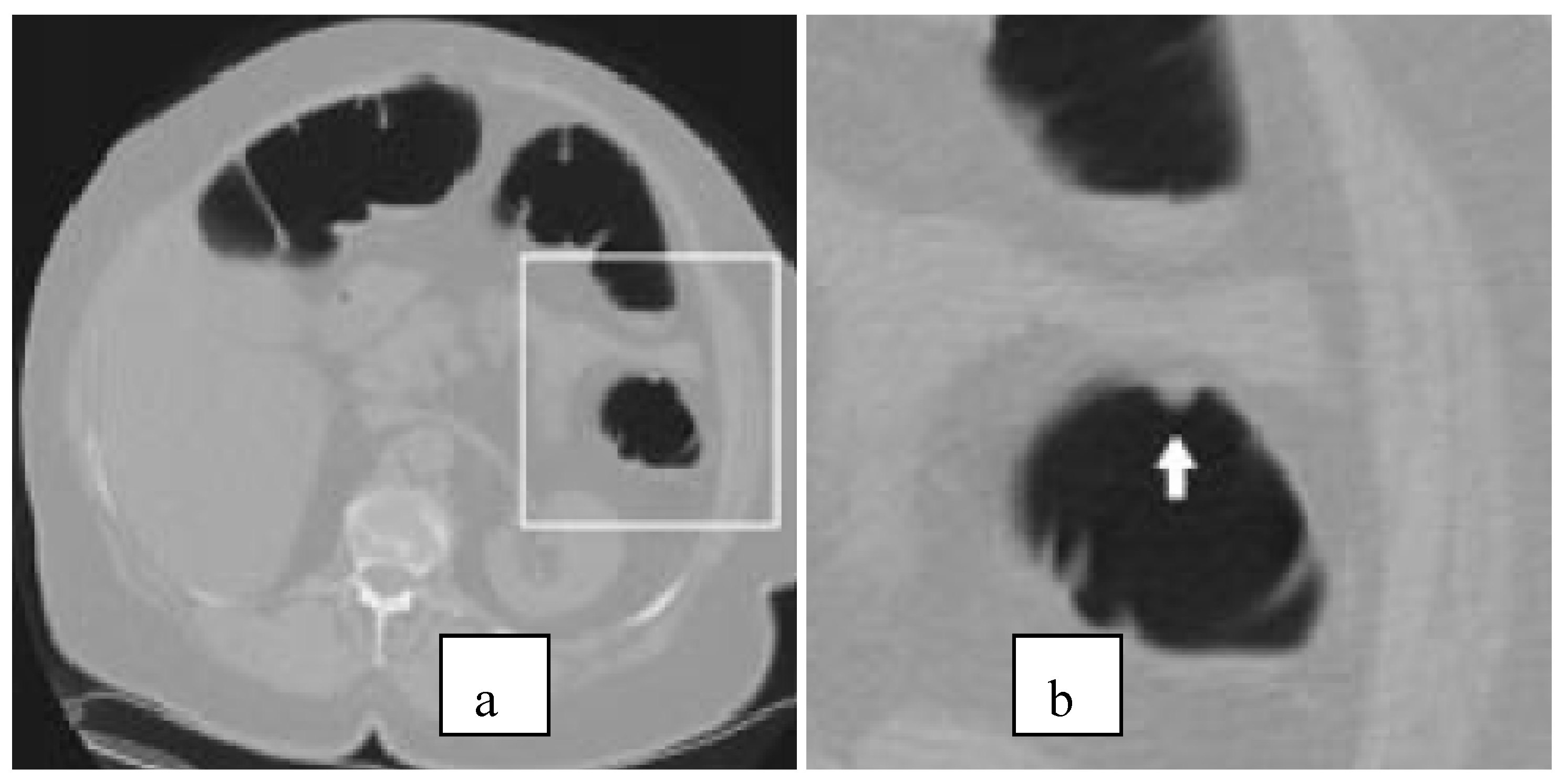
4.1. Data Set Details and Feature Selection

To assess the classification accuracy of WP-SVM, we used volumes of interest (VOIs) representing lesion candidates in clinical CTC data sets. The VOIs were labeled into true polyps (TP) and false positives (FP) by expert radiologists. The CTC data used, was acquired by use of helical single-slice and multi-slice CT scanners (GE HiSpeed CTi, LightSpeed QX/I, and LightSpeed Ultra; GE Medical Systems, Milwaukee, WI). The patients’ colons were prepared with standard laxative pre-colonoscopy cleansing and scanned in supine and prone positions with collimations of 1.25 - 5.0 mm, reconstruction intervals of 1.0 – 5.0 mm, X-ray tube currents of 50 – 260 mAs with 120 – 140 kVp, in-plane voxel sizes of 0.51– 0.94 mm, and a CT image matrix size of 512 x 512. Two CTC scan positions (supine and prone) are generally used for each patient to improve the specificity of polyp detection through improved differentiation of mobile residual stool from polypoid lesions [31, 32]. We further divided the VOIs in the TP class into two categories: medium-size polyps that were between 6-9 mm in size (hereafter, TP1), and large polyps ≥10 mm (hereafter, TP2). This partition was determined by correlating the CTC data with colonoscopy reports. The motivation for this size-based partitioning is that in colorectal screening, large polyps are considered to require polypectomy, whereas for smaller polyps a follow-up surveillance may suffice. A total of 61 colonoscopy-confirmed polyps measured 6 mm or larger: 28 polyps were identified as TP1, and 33 polyps as TP2. The number of entries in the TP class would be higher than the number of actual polyps and this is because the lesion may be seen in both supine and prone positions, and because some large lesions could be represented by more than one detection.

Table 3. Database properties.

Symbol	Name	Count
DB1	Database 1	Class 1 (FP) = 8008 Class 2 (TP1) = 43 Class 3 (TP2) = 84
		VOI=16*16*16=4096 Features

FP: False Positive; TP1: True Positive (medium-size polyps: 6–9 mm); TP2: True Positive (polyps >=10 mm); VOI: Volume of Interest

Table 3. Database properties.

Symbol	Name	Count
DB1	Database 1	Class 1 (FP) = 8008 Class 2 (TP1) = 43 Class 3 (TP2) = 84
		VOI=16*16*16=4096 Features

FP: False Positive; TP1: True Positive (medium-size polyps: 6–9 mm); TP2: True Positive (polyps >=10 mm); VOI: Volume of Interest

To compare the classification performance of WP-SVM with previously published CAD results, and to confine the variability to the classifier method itself, we used the technique proposed by our earlier work in [2]. As for the feature extraction technique, we adopted the 3D CAD scheme also developed earlier in [2] that extracts a thick region encompassing the entire colonic wall in an isotropic CTC volume. Discriminative geometric features (shape index, curvedness, CT value, gradient, gradient concentration, and directional gradient concentration, where each of which is characterized by nine statistics) identify polyps at each voxel of the extracted colon and are used for detecting polyp candidates. Figure 3 (a) represents an axial CT slice where the white box indicates a region of interest with a polyp whereas Figure 3 (b) is a magnification of the region of interest with the polyp indicated by a white arrow. Folds are shown in light gray and colonic wall in dark gray. Suspicious regions identified by connected components are further segmented by use of hysteresis thresholding followed by fuzzy clustering to identify true polyps from non-polyps.

Figure 3. Effect of Shape Index in Differentiating Polyps.

Figure 3. Effect of Shape Index in Differentiating Polyps.

4.2. Performance and validation criteria for WP-SVM

Because ML algorithms have a tradeoff between the classification accuracy on training data and the generalization accuracy on novel data, and because FP occurrences are much more frequent than those of TP1 and TP2, we calculated four performance measurements: the confusion rate (Mis_Err), the True Positive, the True Negative, and the False Positive Ratios. These can be derived from the entries s_ij of the confusion matrix CM:

$$CM=\left[\begin{array}{ccc}{s}_{11}& s_{12}& s_{13}\\ s_{21}& s_{22}& s_{23}\\ s_{31}& s_{32}& s_{33}\end{array}\right]$$

Index i represents the correct class and index j the predicted class. Thus, s_ij represents the number of data belonging to class i that WP-SVM classified as belonging to class j. The True Positive Ratio (TPR), also known as sensitivity, reflects how sensitive WP-SVM is in detecting polyps, whereas the True Negative Ratio (TNR), also referred to as specificity, represents how accurately the classifier identifies false positives. The False Positive Ratio (FPR) is simply the complement of TNR, and Mis_Err is the overall misclassification rate.

$$Mis\_Err=\frac{{\displaystyle \sum _{i=1,i\ne j}^c{s}_{ij}}}{{\displaystyle \sum _{i=1,j=1}^c{s}_{ij}}},TP{R}_i=\frac{s_{ii}}{{\displaystyle \sum _{j=1}^3{s}_{ij}}},TN{R}_j=\frac{s_{jj}}{{\displaystyle \sum _{j=1}^3{s}_{ij}}},\mathrm{and }FPR=1-TNR$$

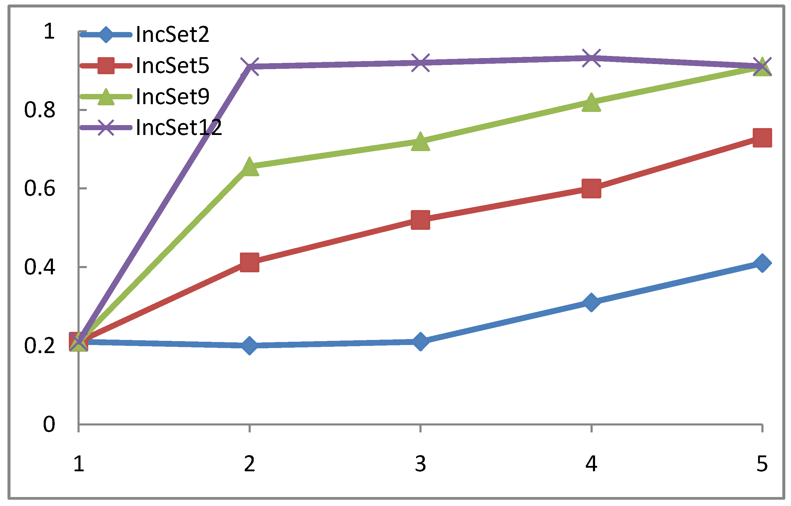
4.3. WP-SVM Performance in Processing Chunk versus Sequential Data

To characterize the detection performance of WP-SVM, we divided DB1 into 3 independent sets of data: a training set (hereafter, TrainSet), a testing set (hereafter, TestSet), and an incremental set (hereafter, IncSet) in a manner to preserve all data that belong to a patient in one of these sets. This validation technique insures exclusion of any criterion that has been optimized during the model training phase from optimistically biasing the model generalization performance in the validation step. We compared CTC classification performance when the ML model was retrained (hereafter, Retrain_Model) to the case where incremental learning using WP-SVM was applied. In the latter case, the dynamic data were processed either in a chunk manner (hereafter, Inc_Model) and by incorporating the data sequentially into the classifier (hereafter, Inc_Seq_Model). We also compared WP-SVM to the confusion rate for simple incremental SVM as compared to the Retrain_Model. Table 3 summarizes the average result for 20 different experiments as well as CPU requirements as normalized to the baseline of Retrain_Model while using Matlab’s etime routine in order to insure the analysis is independent of machine specifics.

Table 4. Normalized Confusion Rates and CPU Requirements with respect to Retrain_Model for Inc_Model, Inc_Seq_Model, and Incremental SVM.

	Inc_Model	INC_SEQ_MODEL	Incremental SVM
Confusion Rate	1.2	1.07	1.24
CPU Time	0.62	0.675	0.687

Table 4. Normalized Confusion Rates and CPU Requirements with respect to Retrain_Model for Inc_Model, Inc_Seq_Model, and Incremental SVM.

	Inc_Model	INC_SEQ_MODEL	Incremental SVM
Confusion Rate	1.2	1.07	1.24
CPU Time	0.62	0.675	0.687

The ratio of the confusion rates of Inc_Model to the Retrain_Model was found to be 1.2 on average. And for the sequential processing, the ratio of the confusion rates of the WP-SVM to the Retrain_Model was on average improved to a factor of 1.07 - which represents almost a 16% improvement over the chunk data processing scenario. Table 3 also shows the CPU usage times for the models normalized with respect to Initial_Model CPU requirements. On average, the ratio of the CPU times of Inc_Model to the Retrain_Model was 0.401. We also observed a marginal degradation in the CPU time for the Inc_Seq_Model. The ratio of the CPU times of Inc_Seq_Model to the Retrain_Model was 0.675. This means that the improvement in the sequential classifier’s accuracy degraded CPU usage time with respect to batch processing. However, this is a reasonable price to incur for enhancing polyp detection by almost 16% with respect to the batch processing.

To illustrate the advantage of online learning in that incremental training could have the advantage of possibly improving classifier accuracy by being able to incorporate more data into the model over the baseline retrain method., we started with an intentionally poor-performing Initial_Model to which WP-SVM was applied iteratively for testing the model convergence.

Figure 4. TP2 Sensitivity Convergence Rate as a Function of IncSet Sizes.

Figure 4. TP2 Sensitivity Convergence Rate as a Function of IncSet Sizes.

As shown in Figure 4, WP-SVM convergence rate for TP2 in reaching an acceptable sensitivity level is basically influenced by the size of IncSet. With larger IncSet sizes successively applied to Initial_Model, WP-SVM adjusted faster the hyper-plane positions to gradually learn classification of the CTC data without having to consume resources for retraining thus validating the viability of incremental learning in improving model parameters after some iterative training.

4.4. WP-SVM Specificity and Storage Requirements

Because CTC CAD data are often highly unbalanced with respect to the size of the classes TP1, TP2, and FP, the confusion rate does not fully demonstrate the effectiveness of WP-SVM, we therefore investigated the sensitivity of WP-SVM in detecting polyps while the penalty factors ζ and λ were varied. The main fallout in classification accuracy occurred between classes TP1 and TP2. The WP-SVM identified the FP class correctly but failed to reach 100% detection sensitivity in the classes TP1 and TP2. This is not surprising considering that these classes are not completely linearly separable and that kernel functions were not used in mapping the input feature space in the SVM procedure. Figure 5 compares the performance of Inc_Model and Retrain_Model in terms of receiver operating characteristic (ROC) curves. The curves depict the trade-off between the TPR and FPR rates for TP1, TP2, and FP.

Figure 5. FP, TP2 and TP1 ROC Curves for Retrain_Model and Inc_Model.

Figure 5. FP, TP2 and TP1 ROC Curves for Retrain_Model and Inc_Model.

Figure 5 indicates that as TPR increases, FPR increases as well because the FPR which makes WP-SVM a good decision method will simultaneously have a reasonably high detection sensitivity and specificity for a specific setting of ζ. Since WP-SVM reached a sensitivity of 91 % and 96 % for TP1 and TP2 with a specificity of 90.3% and 90 % and an average of 3.2 false positive per patient respectively. Since the area under the ROC curve of WP-SVM is greater than the area under a hypothetical diagonal line which would represent a random guess, we can conclude that the obtained WP-SVM ROC curves are informative and that WP-SVM presents a promising online learning algorithm for detecting polyps.

Table 5. Binary and Offline CAD Results as Reported in Literature Compared with WP-SVM.

Reference	Results	Settings
[33]	95%, average of 1.5 false positive per patient	72 patients, 144 data sets, 21 polyps >=5 mm in 14 patients
[34]	90.5%, average of 2.4 false positive per patient	121 patients, 242 data sets, 42 polyps >=5 mm in 28 patients
[35]	80%, average of 8.2 false positive per patient	18 patients, 15 polyps >= 5mm in 9 patients
[36]	100%, average of 7 false positive per patient	8 patients, 7 polyps>=10 mm in 4 patients
	50%, average of 7 false positive per patient	8 patients, 11 polyps measuring between 5 – 9 mm in 3 patients
[37]	90%, average of 15.7 false positive per patient	40 patients, 80 data sets,39 polyps>=3 mm in 20 patients
WP-SVM	93.4% average of 3.2 false positive per patient	169 patients, 28 polyps measuring between 6-9 mm and 33 polyps >10mm

Table 5. Binary and Offline CAD Results as Reported in Literature Compared with WP-SVM.

Reference	Results	Settings
[33]	95%, average of 1.5 false positive per patient	72 patients, 144 data sets, 21 polyps >=5 mm in 14 patients
[34]	90.5%, average of 2.4 false positive per patient	121 patients, 242 data sets, 42 polyps >=5 mm in 28 patients
[35]	80%, average of 8.2 false positive per patient	18 patients, 15 polyps >= 5mm in 9 patients
[36]	100%, average of 7 false positive per patient	8 patients, 7 polyps>=10 mm in 4 patients
	50%, average of 7 false positive per patient	8 patients, 11 polyps measuring between 5 – 9 mm in 3 patients
[37]	90%, average of 15.7 false positive per patient	40 patients, 80 data sets,39 polyps>=3 mm in 20 patients
WP-SVM	93.4% average of 3.2 false positive per patient	169 patients, 28 polyps measuring between 6-9 mm and 33 polyps >10mm

On average, detection performance reported by the CAD schemes used for binary classification in a non–dynamic scheme, as shown in Table 5, has varied between 50% and 100% with 1.5 to 15.7 false positives per patient. The WP-SVM results for false-positive findings per patient compares favorably with these published results, especially when we consider that WP-SVM is being applied as an online multi-classifier on a larger database. Note that mutli-classification accuracy is expected to be negatively impacted in comparison to binary classification. The parametric model of the SVM allows for adjustments when constructing the discriminant function. However, for multiclass problems these parameters do not always exhibit a perfect fit across the entire data set. This is partly supported by the fact that the VC dimension “h” impacts the generalization error and is bounded by the slope of the hyperplane w and R the radius of the smallest sphere that contains all the training points according to [28]: $h<\frac{R^2}{{\Vert w\Vert }^2}$

Finally, Table 6 compares the storage requirements of the Retrain_Model vs. the Inc_model when WP-SVM is applied. Over time, as the polyps’ database increases, computer storage for the Retrain_Model will require memory space proportional to the number of CTC acquired so that the model can be retrained each time a new CTC is acquired. For the Inc_model, the memory space is reduced to the number of features f multiplied by the number of different classes.

Table 6. Storage Requirements.

Classifier Type	Data Structure Size
Retrain_Model	1- a permanent storage of size (N+incnum)*f that is always increasing.
Inc_Model	1- f by c for classifier parameters 2-temporary memory of size incnum*f for dynamic data if classifier is not updated.

incnum= number of dynamic data acquired

Table 6. Storage Requirements.

Classifier Type	Data Structure Size
Retrain_Model	1- a permanent storage of size (N+incnum)*f that is always increasing.
Inc_Model	1- f by c for classifier parameters 2-temporary memory of size incnum*f for dynamic data if classifier is not updated.

incnum= number of dynamic data acquired

5. Conclusions

We presented a novel extension to LS-SVM to provide a dynamic multiclassification framework for CTC classification. The ratio of the confusion rates of Inc_Seq_Model and Retrain_Model was 1.07 on average, and the CPU requirements of the WP-SVM were 0.675 times the Retrain_Model. The accuracy of the proposed model was more constrained by the initial model accuracy when chunk learning rather than iterative learning was applied. Performance evaluation based on 169 clinical CTC cases showed using a 3D computer-aided diagnosis (CAD) scheme for feature reduction polyp detection sensitivities of 91% and 96% for 6 – 9 mm and ≥10 mm polyps with specificities of 90.3% and 90%, respectively. We also showed that the storage requirements of WP-SVM are drastically reduced compared to standard classification, and that this is due to the fact that only the hyper-plane parameters are required for updating the classifier. The experimental results demonstrate the capability of WP-SVM in detecting polyps and motivate further work to improve performance accuracy and specificity measures as well as to validate the detection rates on a larger TP database. Further developments will include the application of kernel methods to WP-SVM and an adaptation of SVM as an image preprocessing technique for feature extraction. The future work will also involve the validation of the WP-SVM over a wider range of TP subclasses such as pedunculated, sessile, and flat polyps, and over a wider range of FP subclasses such as folds, stool, and tagged materials.

References and Notes

1. Macari, M.; Bini, E.J. CT Colonography: Where Have We Been And Where Are We Going? Radiology 2005, 237, 819–833. [Google Scholar]
2. Yoshida, H.; Näppi, J. Three-Dimensional Computer-Aided Diagnosis Scheme for Detection of Colonic Polyps. IEEE T. Med. Imaging 2001, 20, 1261–1274. [Google Scholar]
3. Duda, R.; Hart, P.; Stork, D. Pattern Classification, 2nd Ed. ed; John Wiley & Sons: New York, NY, USA, 2001. [Google Scholar]
4. Cristianini, N.; Shawe-Taylor, J. An Introduction To Support Vector Machines And Other Kernel-Based Learning Methods; Cambridge University Press: New York, NY, USA, 2000; pp. 64–87. [Google Scholar]
5. Basu, S.; Bilenko, M.; Banerjee, A.; Mooney, R. Probabilitic Semi-Supervised Clustering With Constraints, in Semi-Supervised Learning; Chapelle, O., Scholkopf, B., Zien, A., Eds.; The MIT Press: New York, NY, USA, 2006; p. 72. [Google Scholar]
6. Zou, A.; Wu, F.X.; Ding, J.R.; Poirier, G.G. Quality Assessment Of Tandem Mass Spectra Using Support Vector Machine. BMC Bioinformatics 2009, 10 Suppl. 1. [Google Scholar]
7. Isa, D.; Lee, L.H.; Kallimani, V.P.; RajKumar, R. Text Document Preprocessing with the Bayes Formula for Classification Using the Support Vector Machine. IEEE T. Knowl. Data En. 2008, 20, 1264–1272. [Google Scholar] [CrossRef]
8. Zhang, L.; Wei, Y.; Wang, Z. Prediction on Ecological Water Demand Based on Support Vector Machine. International Conference on Computer Science and Software Engineering 2008, 5, 1032–1035. [Google Scholar]
9. Chen, S.H. A Support Vector Machine Approach For Detecting Gene-Gene Interaction. Genet. Epidemiol. 2007, 32, 152–167. [Google Scholar] [CrossRef] [PubMed]
10. Yao, X.; Tham, L.G.; Dai, F.C. Landslide Susceptibility Mapping Based on Support Vector Machine: A Case Study On Natural Slopes of Hong Kong, China. Geomorphology 2008, 101, 572–582. [Google Scholar] [CrossRef]
11. Cheng, J.; Baldi, P. Improved Residue Contact Prediction Using Support Vector Machines And A Large Feature Set. BMC Bioinformatics 2007, 8, 113. [Google Scholar] [CrossRef] [PubMed]
12. Ribeiro, B. Support Vector Machines For Quality Monitoring In A Plastic Injection Molding Process. IEEE T. Syst. Man Cy. C 2005, 35, 401–410. [Google Scholar] [CrossRef]
13. Valentini, G. An Experimental Bias-Variance Analysis of SVM Ensembles Based on Resampling Techniques. IEEE T. Syst. Man Cy. B 2005, 35, 1252–1271. [Google Scholar] [CrossRef]
14. Waring, C.; Liu, X. Face Detection Using Spectral Histograms and SVMs. IEEE T. Syst. Man Cy. B 2005, 35, 467–476. [Google Scholar] [CrossRef]
15. Chakrabartty, S.; Cauwenberghs, G. Sub-Microwatt Analog VLSI Support Vector Machine for Pattern Classification and Sequence Estimation. Adv. Neural Information Processing Systems (NIPS'2004) 2005, 17. [Google Scholar]
16. Dacheng, T.; Tang, X.; Li, X.; Wu, X. Asymmetric Bagging and Random Subspace for Support Vector Machines-Based Relevance Feedback in Image Retrieval. IEEE T. Pattern Anal. 2006, 28, 1088–1099. [Google Scholar] [CrossRef] [PubMed]
17. Dong, J.X.; Krzyzak, A.; Suen, C.Y. Fast SVM Training Algorithm With Decomposition On Very Large Data Sets. IEEE T. Pattern Anal. 2005, 27, 1088–1099. [Google Scholar]
18. Mao, K. Feature Subset Selection For Support Vector Machines Through Discriminative Function Pruning Analysis. IEEE T. Syst. Man Cy. B 2004, 34, 60–67. [Google Scholar] [CrossRef]
19. Fung, G.; Mangasarian, O. Proximal Support Vector Machine Classifiers. In Proceedings of the 7th ACM SIGKDD, International Conference on Knowledge Discovery and Data Mining, San Francisco, CA, USA, August 26–29, 2001; pp. 77–86.
20. Song, Q.; Hu, W.; Xie, W. Robust Support Vector Machine With Bullet Hole Image Classification. IEEE T. Syst. Man Cy. C 2002, 32, 440–448. [Google Scholar] [CrossRef]
21. Hua, S.; Sun, Z. A Novel Method of Protein Secondary Structure Prediction With Light Segment Overlap Measure: Support Vector Machine Approach. J. Mol. Biol. 2001, 308, 397–407. [Google Scholar] [CrossRef] [PubMed]
22. Matas, J.; Li, Y. P.; Kittler, J.; Jonsson, K. Support Vector Machines For Face Authentication. Image Vis. Comput. 2002, 20, 369–375. [Google Scholar]
23. Chiu, D.Y.; Chena, P.J. Dynamically Exploring Internal Mechanism of Stock Market by Fuzzy-Based Support Vector Machines With High Dimension Input Space and Genetic Algorithm. IEEE Expert 2009, 36, 1240–1248. [Google Scholar] [CrossRef]
24. Guoa, X.; Yuan, Z.; Tian, B. Supplier Selection Based On Hierarchical Potential Support Vector Machine. IEEE Expert 2009, 36, 6978–6985. [Google Scholar]
25. Yu, L.; Chen, H.; Wang, S.; Lai, K.K. Evolving Least Squares Support Vector Machines for Stock Market Trend Mining. IEEE T. Evolut. Comput. 2009, 13, 87–102. [Google Scholar]
26. Gao, Z.; Lu, G.; Gu, D. A Novel P2P Traffic Identification Scheme Based on Support Vector Machine Fuzzy Network. Knowledge Discovery and Data Mining 2009, 909–912. [Google Scholar]
27. Diehl, C.; Cauwenberghs, G. SVM Incremental Learning, Adaptation and Optimization. Proceedings of the International Joint Conference on Neural Networks 2003, 4, 2685–2690. [Google Scholar]
28. Vapnik, V. H. The Nature of Statistical Learning Theory, 2nd Ed. ed; Springer: New York, NY, USA, 2000. [Google Scholar]
29. Hsu, C.; Lin, C. A Comparison of Methods For Multi-Class Support Vector Machines. IEEE T. Neural Networ. 2002, 13, 415–425. [Google Scholar]
30. Golub, G.H.; Van Loan, C.F. Matrix Computations; John Hopkins University Press: London, UK, 1996. [Google Scholar]
31. Chen, S. C.; Lu, D.S.; Hecht, J. R. CT Colonography: Value of Scanning in Both the Supine and Prone Positions. AJR 1999, 172, 595–599. [Google Scholar] [CrossRef] [PubMed]
32. Nappi, J.; Okamura, A.; Frimmel, H.; Dachman, A.H.; Yoshida, H. Region Based Supine-Prone Correspondence For The Reduction Of False-Positive Cad Polyp Candidates in CT Colonography. ACAD Radiol. 2005, 12, 695–707. [Google Scholar] [CrossRef] [PubMed]
33. Nappi, J.; Yoshida, H. Feature-Guided Analysis For Reduction of False Positives in Cad of Polyps for Computed Tomographic Colonography. Med. Phys. 2003, 30, 1592–1601. [Google Scholar] [CrossRef] [PubMed]
34. Kiss, G.; Cleynenbreugel, J.; Thomeer, M.; Suetens, P.; Marchal, G. Computer–aided Diagnosis in Virtual Colonography Via Combination of Surface Normal and Sphere Fitting Methods. Eur. Radiol. 2002, 12, 77–81. [Google Scholar] [CrossRef] [PubMed]
35. Paik, D.S.; Beaulieu, C.F.; Rubin, G.D.; Acar, B.; Jeffrey, R.B., Jr.; Yee, J.; Dey, J.; Napel, S. Surface Normal Overlap: a Computer Aided Detection Algorithm with Application to Colonic Polyps and Lung Nodules in Helical CT. IEEE Trans. Med. Imaging 2004, 23, 661–675. [Google Scholar] [CrossRef] [PubMed]
36. Jerebko, A.K.; Summers, R.M.; Malley, J.D.; Franaszek, M.; Johnson, C.D. Computer Assisted Detection of Colonic Polyps with CT Colonography Using Neural Networks and Binary Classification Trees. Med. Phys. 2003, 30, 52–60. [Google Scholar] [CrossRef] [PubMed]
37. Masutani, Y.; Yoshida, H.; MacEneaney, P.; Dachman, A. Automated Segmentation of Colonic Walls for Computerized Detection of Polyps in CT Colonography. J. Comput. Assist. Tomogr. 2001, 25, 629–638. [Google Scholar] [CrossRef]