Recognition of Pulmonary Nodules in Thoracic CT Scans Using 3-D Deformable Object Models of Different Classes

Abstract

The present paper describes a novel recognition method of pulmonary nodules (i.e., cancer candidates) in thoracic computed tomography scans by use of three-dimensional spherical and cylindrical models that represent nodules and blood vessels, respectively. The anatomical validity of these object models and their fidelity to computed tomography scans are evaluated based on the Bayes theorem. The nodule recognition is employed by the maximum a posteriori estimation. The proposed method is applied to 26 actual computed tomography scans, and experimental results are shown.

1. Introduction

Lung cancer is the most common cause of death among all cancers worldwide [1]. To cope with this serious situation, mass screening for lung cancer has been widely performed by simple X-ray films with sputum cytological tests. However, it is known that the accuracy of this method is not sufficient for the early detection of lung cancer [2,3]. Therefore, a lung cancer screening system by computed tomography (CT) for mass screening is proposed [4]. This system improves the accuracy of the cancer detection considerably [5], but has one problem that the number of the images is increased to over dozens of slice sections per patient from 1 X-ray film. It is difficult for a radiologist (i.e., a medical doctor who specializes in reading radiographs) to interpret all the images in a limited time. In order to make the system more practical, it is necessary to build a computer-aided diagnosis (CAD) system that automatically detects abnormal regions suspected to comprise pulmonary nodules that are the major radiographic indicators of lung cancers, and informs a radiologist of their positions in CT scans as a second opinion.

Extensive research has been dedicated to automated detection of pulmonary nodules in thoracic CT scans [6]. Morphological [7] image filters [8,9,10] are conventional approaches. In the work [11], a multiple-thresholding technique was used to detect nodules that had peaked intensity distribution. Hessian-based image filters [12,13] individually enhanced blob- and ridge-shaped regions that corresponded to nodules and blood vessels, respectively. These methods were often used for initial detection of nodules, and were intentionally adjusted to minimize the number of misdetection. Consequently, they yielded many false candidates called false positives (FP) that corresponded to normal pulmonary structures such as blood vessels.

In order to reduce false positives, feature-based discrimination methods between nodules and false positives have been also developed [14,15,16,17,18,19]. Kawata et al. reported a classification method [20] of nodules based on differences in shape indexes, which were computed from two principal curvatures of intensity profiles in images, between nodules and false positives. Suzuki et al. proposed a method [21] that suppressed false positives by using voxel values in regions of interest as input for a novel artificial neural network [22].

Model-based methods are the promising approaches as well. Several works with nodule models were reported. Lee et al. [23] proposed a template-matching method using nodular models with two-dimensional (2-D) Gaussian distribution as reference images to CT scans. The method had an advantage of being able to use the geometrical features of nodules as well as gray level features. Ozekes et al. [24] designed a 3-D prismatic nodule template that was composed of several layered matrices. Farag et al. [25] developed 3-D deformable nodule models such as spherical models of various radii. These methods can make use of the characteristics of the 3-D relation between a suspicious region in a slice section and the other regions in the adjacent slice sections.

Not only nodules but also normal pulmonary structures were modeled in a study reported by McCulloch et al. [26]. A ribbon model, for example, was used for representing a blood vessel region in a slice section. Based on the Bayes theorem, the probabilities of the models were calculated from image features such as step-edges extracted by the Canny edge detector. The most likely model was determined by the maximum a posteriori (MAP) estimation. In this study, by using the models, the anatomical knowledge on the normal structures of human organs can be introduced into recognition of diseases, but only 2-D models and image features were used.

In the present paper, we propose a novel recognition method of pulmonary nodules in thoracic CT scans by use of 3-D deformable spherical and cylindrical models that represent nodules and blood vessels, respectively. The anatomical validity of these object models are evaluated by the predefined probability distributions of their parameters. The fidelity of the object models to CT scans are also evaluated based on the differences in intensity distributions between the CT scans and templates produced from the object models. Through these evaluations, the posteriori probabilities of hypotheses that the object models appear in the CT scans are calculated by use of the Bayes theorem. The nodule recognition is employed by the MAP estimation.

One of the major contribution of the present paper is to enable the computers to make use of the 3-D anatomical knowledge of both lesions and normal structures in organs by use of the 3-D object models. The 3-D knowledge is more informative than the 2-D knowledge, and thereby the ability to use the 3-D knowledge is an advantage of the proposed method. The other is to formulate the 3-D model-based Bayes inference so that it can be applied to 3-D CT volume data. The Bayes inference uses both the anatomical knowledge and the CT data, and thus, even if they comprise uncertainty, it can achieve more accurate recognition by complementing them mutually.

2. Overview of the Proposed Method

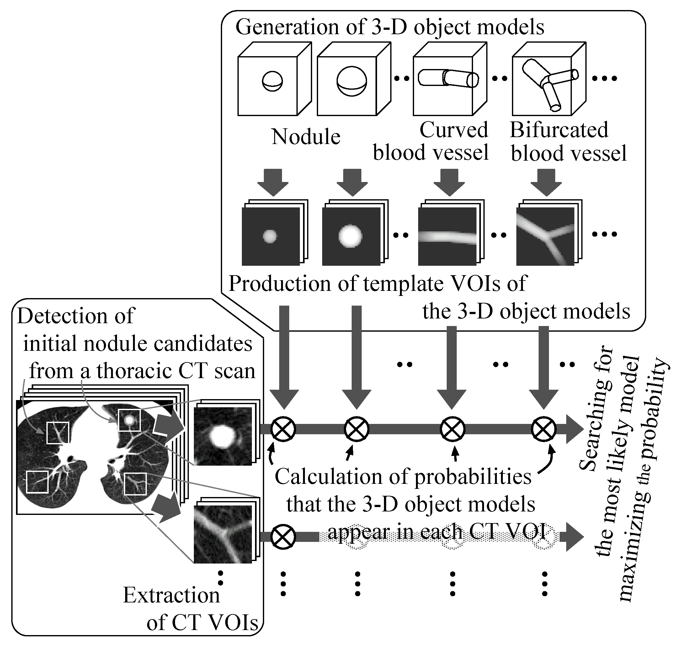
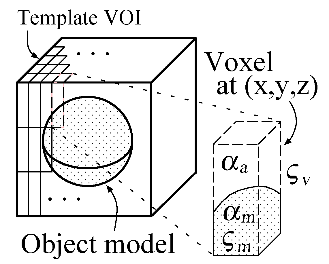
Figure 1 illustrates the overview. First, initial nodule candidates are detected from individual slice sections of a thoracic CT scan by our previous detection methods [8,27,28], and then square areas of a certain size are settled on the slice sections so as to comprise the nodule candidates. White squares on a slice section in the leftmost box in the figure show examples of such square areas. Additional isometric square areas are settled at the same X–Y positions on the adjacent slice sections. These square areas are formed into volumes of interest (VOIs) in the CT scans.

Figure 1. The process of the proposed method.

Figure 1. The process of the proposed method.

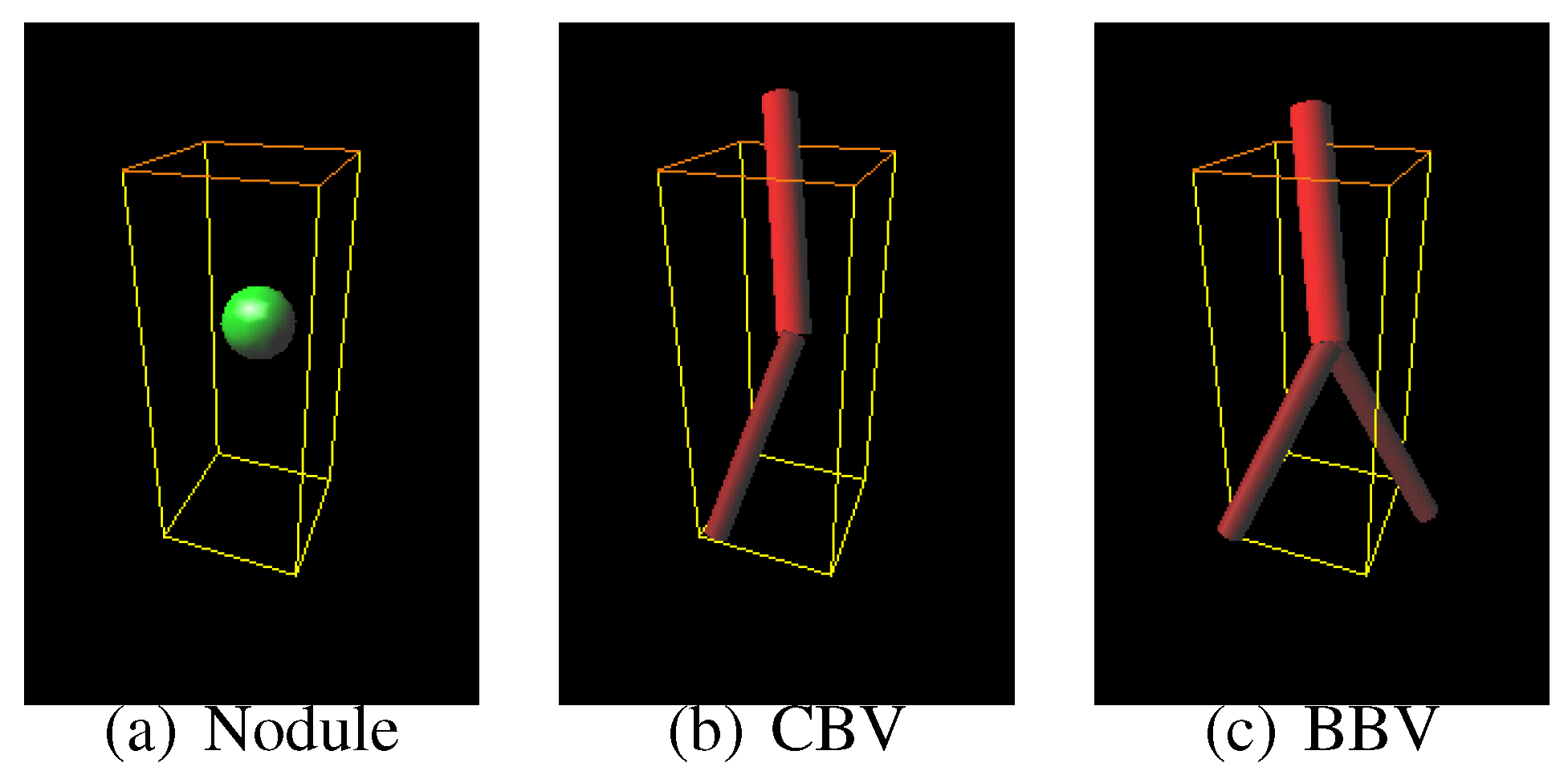
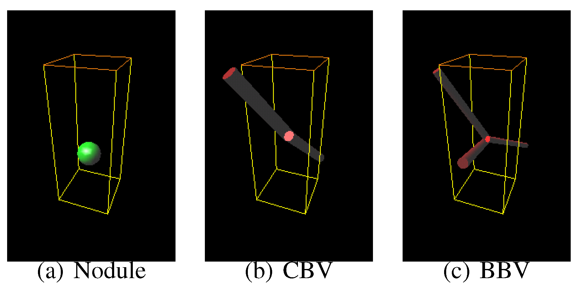
Sphere and connected-cylinder models, that represent nodules and blood vessels, respectively, are generated as shown in the topmost box. These object models can be deformed by changing their parameters such as the radius of the sphere model. Template VOIs are produced by projecting the object models onto them.

The template VOIs are matched to each VOI in the CT scans, and the posteriori probabilities of hypotheses that the CT VOI arises from the object models are calculated using the Bayes theorem. The most likely object model is searched for by the MAP estimation with an optimization method. The CT VOI is determined to be abnormal if the most likely object model is the nodule model, and vice versa.

3. 3-D Deformable Object Models

Our preliminary study [29] indicated that the 64% of false positives originate from blood vessels in lungs. Hence, discrimination between nodules and blood vessels has been the most important issue. To solve the issue, we focus on analyzing differences in 3-D shape between them from the anatomical point of view. Nodules appear as sphere-like masses in lungs, especially when they are in the early stages of diseases. Therefore, they tend to be observed as isolated circle-like regions on slice sections. In contrast, blood vessels make 3-D tree structures in lungs and are observed as thin regions that are connected with each other. To analyze their shapes, we represent nodules and blood vessels as 3-D geometric figures that can be deformed by changing their parameters. The anatomical validity of the deformation is quantitatively evaluated by the probability distribution of the parameters.

3.1. Nodule

A nodule is represented as a sphere model as shown in Figure 2(a). The central position, radius and X-ray attenuation (i.e., transparency of X-ray) of the nodule model are denoted by ${\mathit{x}}^N=(x^N,y^N,z^N)$, $r^N$ and ${\alpha }_m^N$, respectively. The X-ray attenuation of the area surrounding the nodule model (such an area is often called an air area) is denoted by ${\alpha }_a^N$.

Figure 2. 3-D deformable object models that represent nodules, curved blood vessels (CBV) and bifurcated blood vessels (BBV), respectively.

Figure 2. 3-D deformable object models that represent nodules, curved blood vessels (CBV) and bifurcated blood vessels (BBV), respectively.

In medical diagnosis, the size of a nodule is the most important indicator to determine the stage of disease. Therefore, the radius $r^N$ is more essential to describe a nodule than the other parameters. In this paper, the former (i.e., $r^N$) and latter are called essential and auxiliary parameters, respectively. A nodule model is denoted by $o^N(r^N;{\mathit{x}}^N,{\alpha }_m^N,{\alpha }_a^N)$, where the essential parameter is placed on the left-hand side of the semicolon. The probability of appearance of the nodule model is defined by

$$\begin{array}{c}\hfill p\left(o^N(r^N;{\mathit{x}}^N,{\alpha }_m^N,{\alpha }_a^N)\right)=P^N·g(r^N;{\mu }_r^N,{\sigma }_r^N)\end{array}$$

(1)

where $P^N$ is the probability of the set of all possible nodules, and $g(x;{\mu }_x,{\sigma }_x)$ is a Gaussian distribution with a mean ${\mu }_x$ and standard deviation ${\sigma }_x$.

3.2. Curved blood vessel

A curved section in a blood vessel tree is represented as a two-connected-cylinder model as shown in Figure 2(b). The first cylinder corresponds to the parent vessel (indicated by “1” in the figure) that is nearer to a heart in respect of its blood flow, and the second its child vessel (“2”). The radius of the i-th cylinder ($i=1,2$) is denoted by $r_i^{B_c}$, and its zenith and azimuth angles are denoted by ${\theta }_i^{B_c}$ and ${\varphi }_i^{B_c}$, respectively. The connection position of the two cylinders is denoted by ${\mathit{x}}^{B_c}=(x^{B_c},y^{B_c},z^{B_c})$. The X-ray attenuation of the model and that of its surrounding area are denoted by ${\alpha }_m^{B_c}$ and ${\alpha }_a^{B_c}$, respectively. From these parameters, two additional parameters are calculated: a difference in section area between the cylinders, ${\delta }^{B_c}$, and an angle between the cylinders, ${\psi }^{B_c}$. Because the parameters $r_1^B$, ${\delta }^{B_c}$ and ${\psi }^{B_c}$ are more essential to describe a curved blood vessel, the model is denoted by $o^{B_c}(r_1^B,{\delta }^{B_c},$${\psi }^{B_c};{\mathit{x}}^{B_c},r_2^{B_c},$${\theta }_1^{B_c},{\varphi }_1^{B_c},{\theta }_2^{B_c},$ ${\varphi }_2^{B_c},{\alpha }_m^{B_c},{\alpha }_a^{B_c})$.

The probability of appearance of the curved blood vessel model is defined by

$$\begin{array}{ccc}& & p\left(o^{B_c}(r_1^B,{\delta }^{B_c},{\psi }^{B_c};\cdots )\right)\hfill \\ & =& P^{B_c}·g(r_1^B;{\mu }_{r1}^B\left({\mathit{x}}^{B_c}\right),{\sigma }_{r1}^{B_c})·\hfill \\ & & g({\delta }^{B_c};{\mu }_{\delta }^{B_c},{\sigma }_{\delta }^{B_c})·g({\psi }^{B_c};{\mu }_{\psi }^{B_c},{\sigma }_{\psi }^{B_c})\hfill \end{array}$$

(2)

where $P^{B_c}$ is the probability of the set of all possible curved sections in blood vessel trees.

In Equation (2), the mean radius of blood vessels ${\mu }_{r1}^B\left({\mathit{x}}^{B_c}\right)$ is defined as being the function of the position ${\mathit{x}}^{B_c}$ so as to represent a relation between the radius and position in a lung. Generally, blood vessels are thick in the central area of a lung, and they become thinner as they approach the peripheral area. The relation is formulated by

$${\mu }_{r1}^B\left({\mathit{x}}^{B_c}\right)={\kappa }_1^{B}exp\left(-{\kappa }_2^B·|{\mathit{x}}^{B_c}-{\mathit{c}}^L|\right)$$

(3)

where ${\mathit{c}}^L$ is the central position of the boundary box that circumscribes a lung, $|\mathit{x}-\mathit{c}|$ is the distance between $\mathit{x}$ and $\mathit{c}$. The coefficient values ${\kappa }_1^B$ and ${\kappa }_2^B$ are constant.

In our previous study [30], we investigated statistical relations between the radii and positions of blood vessels in lung regions from population data, and obtained the 3-D distribution of the blood vessel radii. From several functions, the exponential function represented in Equation (3) is selected as the best-fit one to the distribution, and the coefficient values ${\kappa }_1^B$ and ${\kappa }_2^B$ are determined from the fitting result.

3.3. Bifurcated blood vessel

A bifurcation in a blood vessel tree is represented as a three-connected-cylinder model as shown in Figure 2(c).

The probability of appearance of a bifurcated blood vessel model $o^{B_b}(r_1^{B_b},{\delta }_{23}^{B_b},$ ${\delta }_{123}^{B_b},{\psi }_{12}^{B_b},{\psi }_{13}^{B_b},$ ${\psi }_{23}^{B_b};\cdots )$ is defined in the same manner as a curved blood vessel as follows:

$$\begin{array}{ccc}& & p\left(o^{B_b}(r_1^{B_b},{\delta }_{23}^{B_b},{\delta }_{123}^{B_b},{\psi }_{12}^{B_b},{\psi }_{13}^{B_b},{\psi }_{23}^{B_b};\cdots )\right)\hfill \\ & =& P^{B_b}·g(r_1^{B_b};{\mu }_{r1}^B\left({\mathit{x}}^{B_b}\right),{\sigma }_{r1}^{B_b})·\hfill \\ & & g({\delta }_{23}^{B_b};{\mu }_{\delta 23}^{B_b},{\sigma }_{\delta 23}^{B_b})·g({\delta }_{123}^{B_b};{\mu }_{\delta 123}^{B_b},{\sigma }_{\delta 123}^{B_b})·\hfill \\ & & g({\psi }_{12}^{B_b};{\mu }_{\psi 12}^{B_b},{\sigma }_{\psi 12}^{B_b})·g({\psi }_{13}^{B_b};{\mu }_{\psi 13}^{B_b},{\sigma }_{\psi 13}^{B_b})·\hfill \\ & & g({\psi }_{23}^{B_b};{\mu }_{\psi 23}^{B_b},{\sigma }_{\psi 23}^{B_b})\hfill \end{array}$$

(4)

where $P^{B_b}$ is the probability of the set of all possible bifurcations in blood vessel trees, ${\delta }_{23}^{B_b}$ is the difference in section area between the two child cylinders, ${\delta }_{123}^{B_b}$ is the difference in section area between the parent and child cylinders, that is ${\delta }_{123}^{B_b}$ = $\pi \left({\left(r_1^{B_b}\right)}^2-{\left(r_2^{B_b}\right)}^2-{\left(r_3^{B_b}\right)}^2\right)$, and ${\psi }_{ij}^{B_b}$ is the angle between the i-th and j-th cylinder ($i,j=1,2,3$, $i\ne j$).

3.4. Appearance probabilities of object model sets

The probabilities of the model sets satisfy the following equation:

$${\displaystyle \sum _{\tau \in \{N,B_c,B_b\}}{P}^{\tau }=1}$$

(5)

where τ represents the class of the object model.

4. Modification of Probability Distributions of 3-D Object Models

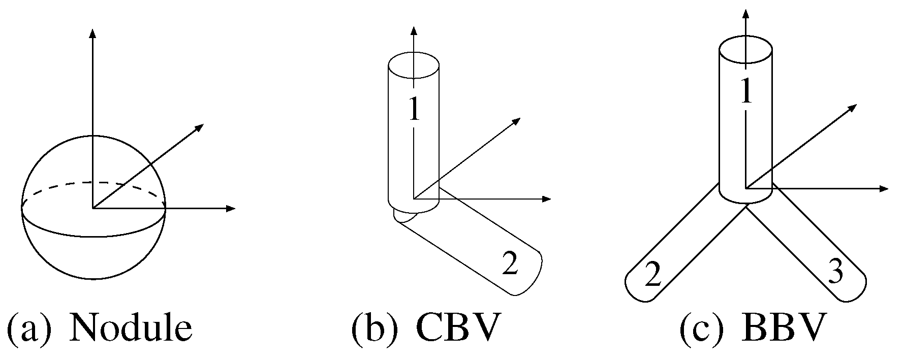
The object models have the different essential parameters in number and type. For example, the nodule model has only one essential parameter $r^N$, whereas the bifurcated blood vessel model has six other essential parameters $r_1^{B_b}$, ${\delta }_{23}^{B_b}$, ${\delta }_{123}^{B_b}$, ${\psi }_{12}^{B_b}$, ${\psi }_{13}^{B_b}$ and ${\psi }_{23}^{B_b}$. The differences in number cause a problem that generally, the probabilities of the object models that have more essential parameters are relatively underestimated.

Let us consider an example case where all the standard deviations are 1 and all the set appearance probabilities $P^{\tau }$ are $1/3$. The radius of a nodule model $r^N$ is supposed to be $\mu +3$ and all the essential parameters of a bifurcated blood vessel model are supposed to be μ’s. Their probabilities are calculated as follows:

$$\begin{array}{ccc}\hfill & & p\left(o^{N_{}}\right)=1/3·g{(\mu +3;\mu ,1)}^{}\approx 0.00148\hfill \end{array}$$

(6)

$$\begin{array}{ccc}\hfill & & p\left(o^{B_b}\right)=1/3·(g(\mu ;\mu ,1){)}^6\approx 0.00134\hfill \end{array}$$

(7)

Although the bifurcated blood vessel model has much more likely parameters, its probability is smaller than that of the nodule model.

Here, let us give a more generalized expression to the model probabilities as follows:

$$p\left(o^{\tau }\left({\omega }^{\tau }\right)\right)=P^{\tau }·p\left({\omega }^{\tau }\right)$$

(8)

where $o^{\tau }\left({\omega }^{\tau }\right)$ represents an object model that has an essential parameter vector:

$$\begin{array}{ccc}\hfill {\omega }^{\tau }& =& ({\omega }_1^{\tau }\in {\Omega }_1^{\tau },{\omega }_2^{\tau }\in {\Omega }_2^{\tau },\cdots \hfill \\ & & {\omega }_d^{\tau }\in {\Omega }_d^{\tau },\cdots ,{\omega }_{D^{\tau }}^{\tau }\in {\Omega }_{D^{\tau }}^{\tau })\in {\Omega }^{\tau }\hfill \end{array}$$

(9)

The notation ${\Omega }^{\tau }$ represents the parameter space and $D^{\tau }$ its dimension. For example, $r_1^{B_c}$, ${\delta }^{B_c}$ and ${\psi }^{B_c}$ in Equation (2) correspond to ${\omega }_1^{B_c}$, ${\omega }_2^{B_c}$ and ${\omega }_3^{B_c}$, respectively, and the dimension $D^{B_c}$ is 3. In Equation (8), the auxiliary parameters are omitted for simplicity. The differences in the dimension $D^{\tau }$ between the model classes τ cause underestimation in $p\left({\omega }^{\tau }\right)$.

One solution to correct the underestimation is to use the geometric average of the parameter probability: ${\displaystyle \sqrt[D^{\tau }]{p\left({\omega }^{\tau }\right)}}$, that is adopted in, for example, recognition of language [31] and speech [32]. Because the dimension $D^{\tau }$ is normalized, the underestimation is no longer caused. However, the geometrically averaged probability causes another problem that generally, the integral of its distribution over the parameter space is not one: ${\displaystyle {\int }_{\omega \in {\Omega }^{\tau }}\sqrt[D^{\tau }]{p\left(\omega \right)}d\omega \ne 1}$. 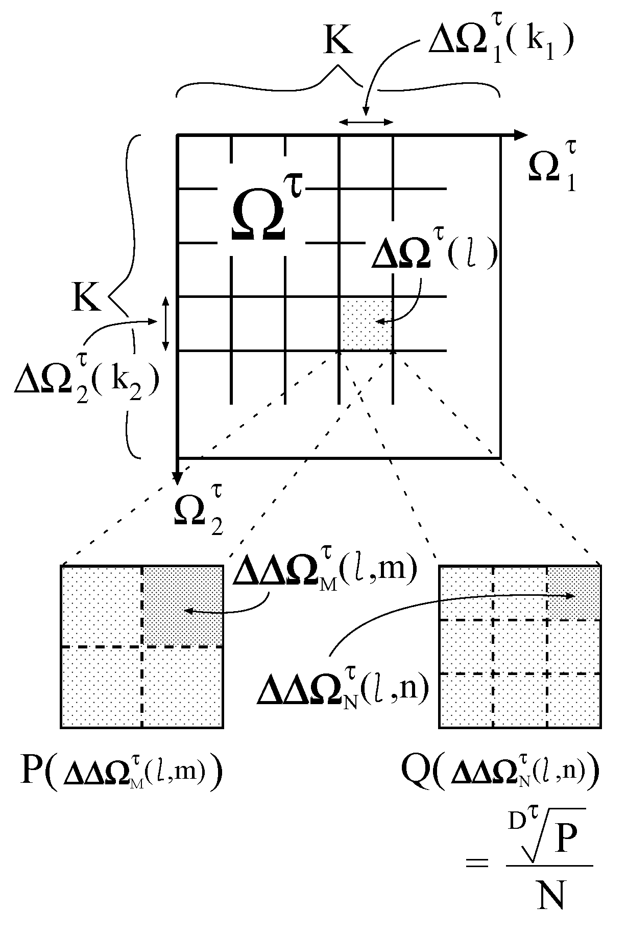We desire a probability distribution that does not cause underestimation and that integrates to one. In this paper, we realize the desired probability distribution on a parameter space that is inhomogeneously divided so that the desired distribution may approximate to the geometrically averaged distribution.

First, each ${\Omega }_d^{\tau }$ is divided into K isometric intervals $\Delta {\Omega }_d^{\tau }\left(k\right)$ ($k=1,2,...,K$) as shown in Figure 3. The interval size $|\Delta {\Omega }_d^{\tau }\left(k\right)|$ is equivalent to $\frac{|{\Omega }_d^{\tau }|}{K}$. By combining $\Delta {\Omega }_d^{\tau }\left(k\right)$, the following subspaces are generated:

$$\begin{array}{c}\hfill \Delta {\Omega }^{\tau }\left(l\right)=\Delta {\Omega }_1^{\tau }\left(k_1\right)\times \Delta {\Omega }_2^{\tau }\left(k_2\right)\times \cdots \times \Delta {\Omega }_{D^{\tau }}^{\tau }\left(k_{D^{\tau }}\right)\end{array}$$

(10)

where $l=1,2,\cdots ,K^{D^{\tau }}$. The operator $A\times B$ yields a product space of A and B. If K is enough large, then the probability distribution $p\left(\omega \right)$ can be regarded as being constant in $\Delta {\Omega }^{\tau }\left(l\right)$. Let $p^{\tau }\left(l\right)$ denote its constant value in $\Delta {\Omega }^{\tau }\left(l\right)$. The probability of $\Delta {\Omega }^{\tau }\left(l\right)$ is calculated as

$$\begin{array}{ccc}& & P\left(\Delta {\Omega }^{\tau }\left(l\right)\right)={\int }_{\Delta {\Omega }^{\tau }\left(l\right)}p\left(\omega \right)d\omega \approx p^{\tau }\left(l\right)·|\Delta {\Omega }^{\tau }\left(l\right)|\hfill \end{array}$$

(11)

Figure 3. Division of a parameter space.

Figure 3. Division of a parameter space.

Then, two types of further division are made for each subspace $\Delta {\Omega }^{\tau }\left(l\right)$. One is the division into $M^{\tau }\left(l\right)$ isometric subsubspaces $\Delta \Delta {\Omega }_M^{\tau }(l,m)$ ($m=1,2,\cdots ,M^{\tau }\left(l\right)$) , and the other is the division into N isometric subsubspaces $\Delta \Delta {\Omega }_N^{\tau }(l,n)$ ($n=1,2,\cdots ,N$). The subsubspace sizes $|\Delta \Delta {\Omega }_M^{\tau }(l,m)|$ and $|\Delta \Delta {\Omega }_N^{\tau }(l,n)|$ are equivalent to $\frac{|\Delta {\Omega }^{\tau }\left(l\right)|}{M^{\tau }\left(l\right)}$ and $\frac{|\Delta {\Omega }^{\tau }\left(l\right)|}{N}$, respectively. The division number N is constant, whereas $M^{\tau }\left(l\right)$ varies with τ and l. Therefore, the parameter space composed of $\Delta \Delta {\Omega }_M^{\tau }(l,m)$ is inhomogeneous. On the inhomogeneously divided parameter space, the desired probability distribution is defined as follows:

$$\begin{array}{ccc}& & P\left(\Delta \Delta {\Omega }_M^{\tau }(l,m)\right)=\frac{P\left(\Delta {\Omega }^{\tau }\left(l\right)\right)}{M^{\tau }\left(l\right)}\hfill \end{array}$$

$$\begin{array}{ccc}& & \approx \frac{p^{\tau }\left(l\right)·|\Delta {\Omega }^{\tau }\left(l\right)|}{M^{\tau }\left(l\right)}=\frac{p^{\tau }\left(l\right)·\left|{\Omega }^{\tau }\right|}{M^{\tau }\left(l\right)·K^{D^{\tau }}}\hfill \end{array}$$

(12)

On the other hand, on the parameter space composed of $\Delta \Delta {\Omega }_N^{\tau }(l,n)$, the geometrically averaged probability distribution is defined as follows:

$$\begin{array}{ccc}& & Q\left(\Delta \Delta {\Omega }_N^{\tau }(l,n)\right)=\frac{\sqrt[D^{\tau }]{P\left(\Delta {\Omega }^{\tau }\left(l\right)\right)}}{N}\hfill \\ & & \approx \frac{1}{N}·\sqrt[D^{\tau }]{p^{\tau }\left(l\right)·|\Delta {\Omega }^{\tau }\left(l\right)|}\hfill \\ & & =\frac{1}{N}·\sqrt[D^{\tau }]{p^{\tau }\left(l\right)·\frac{|{\Omega }^{\tau }|}{K^{D^{\tau }}}}=\frac{\sqrt[D^{\tau }]{p^{\tau }\left(l\right)·\left|{\Omega }^{\tau }\right|}}{N·K}\hfill \end{array}$$

(13)

Because the dimension $D^{\tau }$ is normalized in $\sqrt[D^{\tau }]{p^{\tau }\left(l\right)}$ and $\sqrt[D^{\tau }]{|{\Omega }^{\tau }|}$, the underestimation is not caused in $Q\left(\Delta \Delta {\Omega }_N^{\tau }(l,n)\right)$.

By setting M as follows:

$$M^{\tau }\left(l\right)=⌊N{\left(\frac{p^{\tau }\left(l\right)·\left|{\Omega }^{\tau }\right|}{K^{D^{\tau }}}\right)}^{1-\frac{1}{D^{\tau }}}⌋$$

(14)

with an enough large number N, $P\left(\Delta \Delta {\Omega }_M^{\tau }(l,m)\right)$ approximates to $Q\left(\Delta \Delta {\Omega }_N^{\tau }(l,n)\right)$. In Equation (14), $\lfloor x\rfloor$ is the nearest integer value of x. Consequently, we obtain the probability distribution that suppresses the underestimation and integrates to approximately one.

Let $O^{\tau }(\Delta \Delta {\Omega }_M^{\tau }(l,m))$ denote a set of the object models as follows:

$$\begin{array}{c}\hfill O^{\tau }(\Delta \Delta {\Omega }_M^{\tau }(l,m))=\left\{o^{\tau }\left({\omega }^{\tau }\right)|{\omega }^{\tau }\in \Delta \Delta {\Omega }_M^{\tau }(l,m)\right\}\end{array}$$

(15)

The following probability distribution of the object model set:

$$P\left(O^{\tau }(\Delta \Delta {\Omega }_M^{\tau }(l,m))\right)=P^{\tau }·P\left(\Delta \Delta {\Omega }_M^{\tau }(l,m)\right)$$

(16)

is used instead of $p\left(o^{\tau }\left({\omega }^{\tau }\right)\right)$ as a priori probability distribution in the Bayes formula.

5. Observation Model

The Bayes formula also uses a likelihood function that evaluates the fidelity of an object model to a CT VOI and is defined as the conditional probability of the CT VOI given the object model. To evaluate the fidelity, a template VOI is produced from the object model by simulating the CT imaging process where nodules and blood vessels are observed as regions with particular shapes on CT slice sections. The conditional probability is formulated by use of similarity between the CT VOI and the template VOI.

5.1. Production of templates from 3-D object models

Figure 4 illustrates an object model $o^{\tau }\left({\omega }^{\tau }\right)$ (a nodule model as an example) in 3-D subspace that corresponds to a template VOI of the same size of a CT VOI. Let $v_T(x,y,z;o^{\tau }\left({\omega }^{\tau }\right))$ denote a voxel value at $x,y,z$ in the template VOI. The value is calculated as

$$\begin{array}{c}\hfill v_T\left(x,y,z;o^{\tau }\left({\omega }^{\tau }\right)\right)={\alpha }_m^{\tau }·{\varsigma }_m^{\tau }+{\alpha }_a^{\tau }·({\varsigma }_v-{\varsigma }_m^{\tau })\end{array}$$

(17)

where ${\alpha }_m^{\tau }$ and ${\alpha }_a^{\tau }$ are the X-ray attenuation of the object model and that of its surrounding area, respectively. The notations ${\varsigma }_v$ and ${\varsigma }_m^{\tau }$ are the volume of the whole voxel and that of a part where the object model intersects with the voxel, respectively.

Figure 4. Production of template VOI.

Figure 4. Production of template VOI.

5.2. Likelihood of VOIs to 3-D object models

The fidelity of the object model to a CT VOI is evaluated by the following correlation coefficient between the CT VOI and the template VOI:

$$\begin{array}{ccc}& & \gamma (v_C,v_T)\hfill \\ & & =\frac{{\displaystyle \sum _{x,y,z}(v_C(x,y,z)-{\overline{v}}_C)(v_T(x,y,z)-{\overline{v}}_T)}}{\sqrt{{\displaystyle \sum _{x,y,z}(v_C(x,y,z)-{\overline{v}}_C{)}^2}}\sqrt{{\displaystyle \sum _{x,y,z}(v_T(x,y,z)-{\overline{v}}_T{)}^2}}}\hfill \end{array}$$

(18)

where $v_C(x,y,z)$ is the voxel value at $x,y,z$ in the CT VOI. The notations ${\overline{v}}_C$ and ${\overline{v}}_T$ are the mean voxel values of the CT VOI and template VOI, respectively.

The correlation coefficient $\gamma (v_C,v_T)$ takes a value between 1 and −1. The higher the fidelity is, the larger the correlation coefficient is. The likelihood is defined as

$$p\left(v_C|o^{\tau }\left({\omega }^{\tau }\right)\right)=\frac{\gamma (v_C,v_T)+1}{2}$$

(19)

6. Recognition of Nodules Based on the MAP Estimation

In the MAP estimation, the posteriori probabilities of hypotheses established beforehand are calculated by the Bayes theorem, and the hypothesis with the maximum posteriori probability is adopted as the most likely one.

Given a CT VOI $v_C$, the posteriori probability of the hypothesis that an object model set $O^{\tau }(\Delta \Delta {\Omega }_M^{\tau }(l,m))$ appears in the VOI is defined by

$$\begin{array}{ccc}& & P\left(O^{\tau }(\Delta \Delta {\Omega }_M^{\tau }(l,m))|v_C\right)\hfill \\ & & {\displaystyle ={\int }_{\Delta \Delta {\Omega }_M^{\tau }(l,m)}p\left(o^{\tau }\left(\omega \right)|v_C\right)d\omega }\hfill \\ & & {\displaystyle ={\int }_{\Delta \Delta {\Omega }_M^{\tau }(l,m)}\beta ·p\left(v_C|o^{\tau }\left(\omega \right)\right)p\left(o^{\tau }\left(\omega \right)\right)d\omega }\hfill \end{array}$$

(20)

where $\beta ={\left[p\left(v_C\right)\right]}^{-1}$. In Equation (20), the Bayes formula:

$$p\left(o^{\tau }\left(\omega \right)|v_C\right)=\beta ·p\left(v_C|o^{\tau }\left(\omega \right)\right)p\left(o^{\tau }\left(\omega \right)\right)$$

(21)

is used. Since the size of $\Delta \Delta {\Omega }_M^{\tau }(l,m)$ is small, the likelihood function $p\left(v_C\right|o^{\tau }\left(\omega \right))$ can be regarded as being constant in $\Delta \Delta {\Omega }_M^{\tau }(l,m)$. Thus,

$$\begin{array}{ccc}& & \text{the last term in Equation}\left(20\right)\hfill \\ & & \approx \beta ·p\left(v_C\right|o^{\tau }\left({\check{\omega }}^{\tau }\right)){\int }_{\Delta \Delta {\Omega }_M^{\tau }(l,n)}p\left(o^{\tau }\left(\omega \right)\right)d\omega \hfill \\ & & =\beta ·p\left(v_C\right|o^{\tau }\left({\check{\omega }}^{\tau }\right))P\left(O^{\tau }(\Delta \Delta {\Omega }_M^{\tau }(l,m))\right)\hfill \end{array}$$

(22)

where ${\check{\omega }}^{\tau }$ is a certain essential parameter vector in $\Delta \Delta {\Omega }_M^{\tau }(l,m)$. The likelihood $p\left(v_C\right|o^{\tau }\left({\check{\omega }}^{\tau }\right))$ and the priori probability $P\left(O^{\tau }(\Delta \Delta {\Omega }_M^{\tau }(l,m))\right)$ are obtained from Equation (19) and Equation (16), respectively.

For each class $\tau =\{N,B_c,B_b\}$, the following indices that maximize the posteriori probability:

$$\begin{array}{c}\hfill {\displaystyle (l^{\tau *},m^{\tau *})=arg\underset{l,m}{max}P\left(O^{\tau }(\Delta \Delta {\Omega }_M^{\tau }(l,m))|v_C\right)}\end{array}$$

(23)

are searched for by the Powell method [33]. From the following ratio between the posteriori probabilities:

$$\begin{array}{c}\hfill {\rho }_1\left(v_C\right)=\frac{P\left(O^N(\Delta \Delta {\Omega }_M^N(l^{N*},m^{N*}))|v_C\right)}{{\displaystyle \underset{\tau \ne N}{max}P\left(O^{\tau }(\Delta \Delta {\Omega }_M^{\tau }(l^{\tau *},m^{\tau *}))|v_C\right)}}\end{array}$$

(24)

the CT VOI $v_C$ is determined to be abnormal if ${\rho }_1\left(v_C\right)\ge T_{\rho }$ and to be normal if ${\rho }_1\left(v_C\right)<T_{\rho }$ with a certain threshold $T_{\rho }$.

7. Experimental Results

In this experiment, 26 thoracic CT scans are used with 30 actual pulmonary nodules. They are acquired by the Asterion, TOSHIBA Medical Systems Corporation. The tube current, tube voltage, slice thickness and reconstruction interval are 30 mA, 120 kV, 8 mm and 8 mm, respectively. The CT scans contain from 31 to 44 slice cross sections, each of which has 512 × 512 pixels.

From the CT scans, lung regions are extracted by a threshold-based technique [4], and then initial nodule candidates are detected from the lung regions by our methods [8,27,28]. The number of nodule candidates per scan is 93.8. They are composed of 28 actual nodules (two false negatives occurs) and 92.8 false positives per scan.

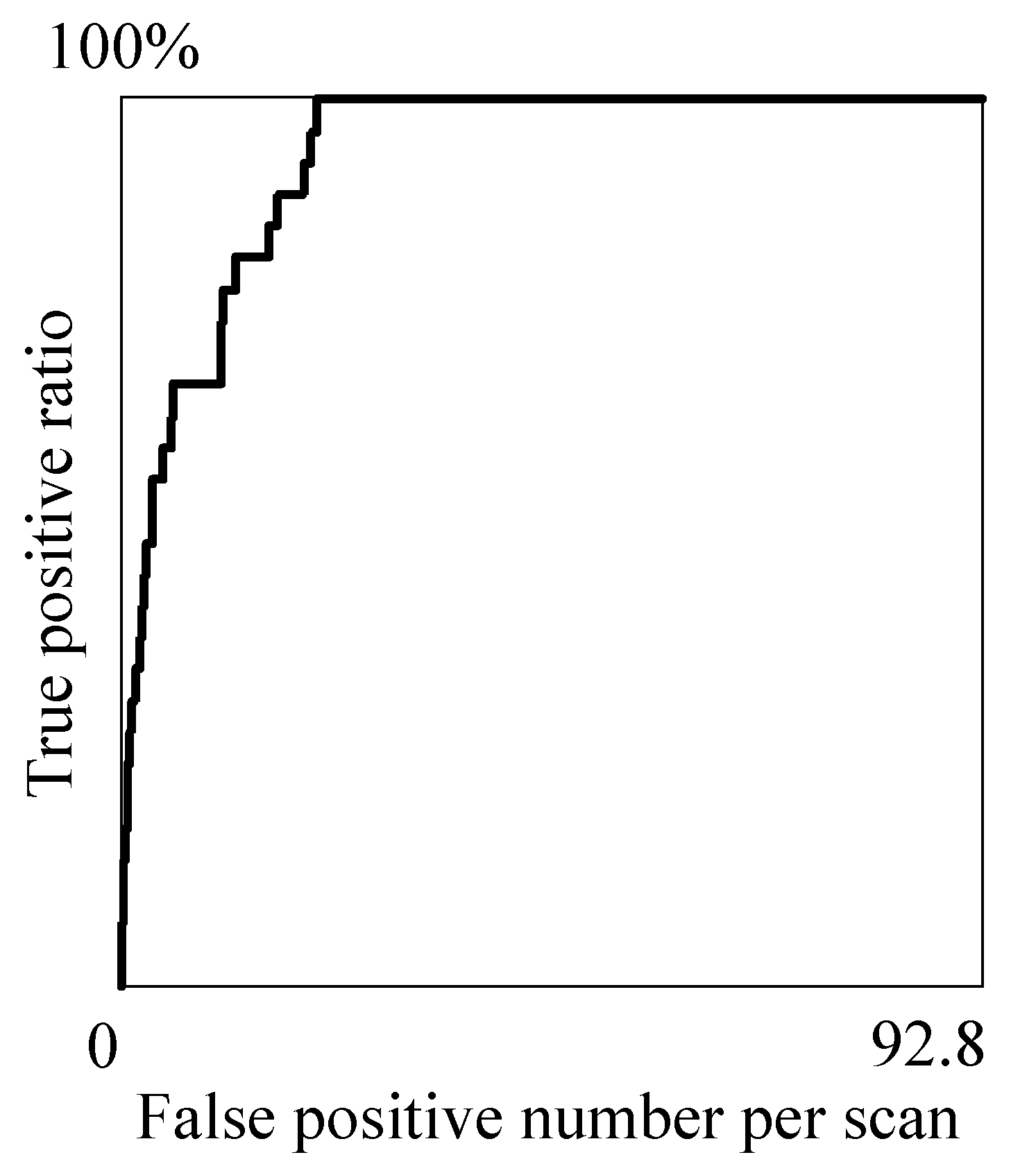
The proposed method is applied to the nodule candidates and, as a final result, Table 1 is obtained that shows the relations between the true positive ratio (TPR) and false positive number per scan (#FP) at the representative threshold values $T_{\rho }$. The relations are depicted by the fROC curve [34] shown in Figure 5. The optimal threshold $T_{\rho }$ is experimentally determined to be 0.954 so as to detect all the true nodules in the candidates and minimize the number of false positives. Table 1 indicates that, by making $T_{\rho }$ less than 0.995, the TPR and #FP can be stably kept more than 82% and less than 22, respectively.

Three cases of the experimental results are examined in detail below.

Table 1. The relations between $T_{\rho }$, TPR and #FP.

$T_{\rho }$	TPR %	#FP
$0.954$	$100.0$	$21.2$
$0.959$	$92.9$	$19.7$
$0.995$	$82.1$	$12.4$
$1.01$	$71.4$	$10.9$
$1.06$	$60.7$	$4.5$
$1.10$	$50.0$	$2.8$

Table 1. The relations between $T_{\rho }$, TPR and #FP.

$T_{\rho }$	TPR %	#FP
$0.954$	$100.0$	$21.2$
$0.959$	$92.9$	$19.7$
$0.995$	$82.1$	$12.4$
$1.01$	$71.4$	$10.9$
$1.06$	$60.7$	$4.5$
$1.10$	$50.0$	$2.8$

Figure 5. The fROC curve of the proposed method.

Figure 5. The fROC curve of the proposed method.

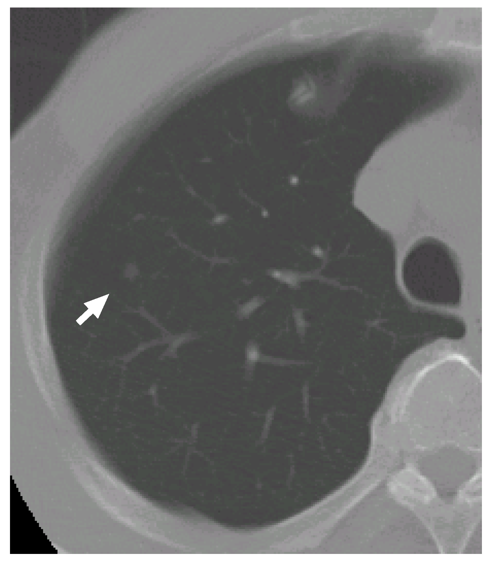
7.1. Case 1

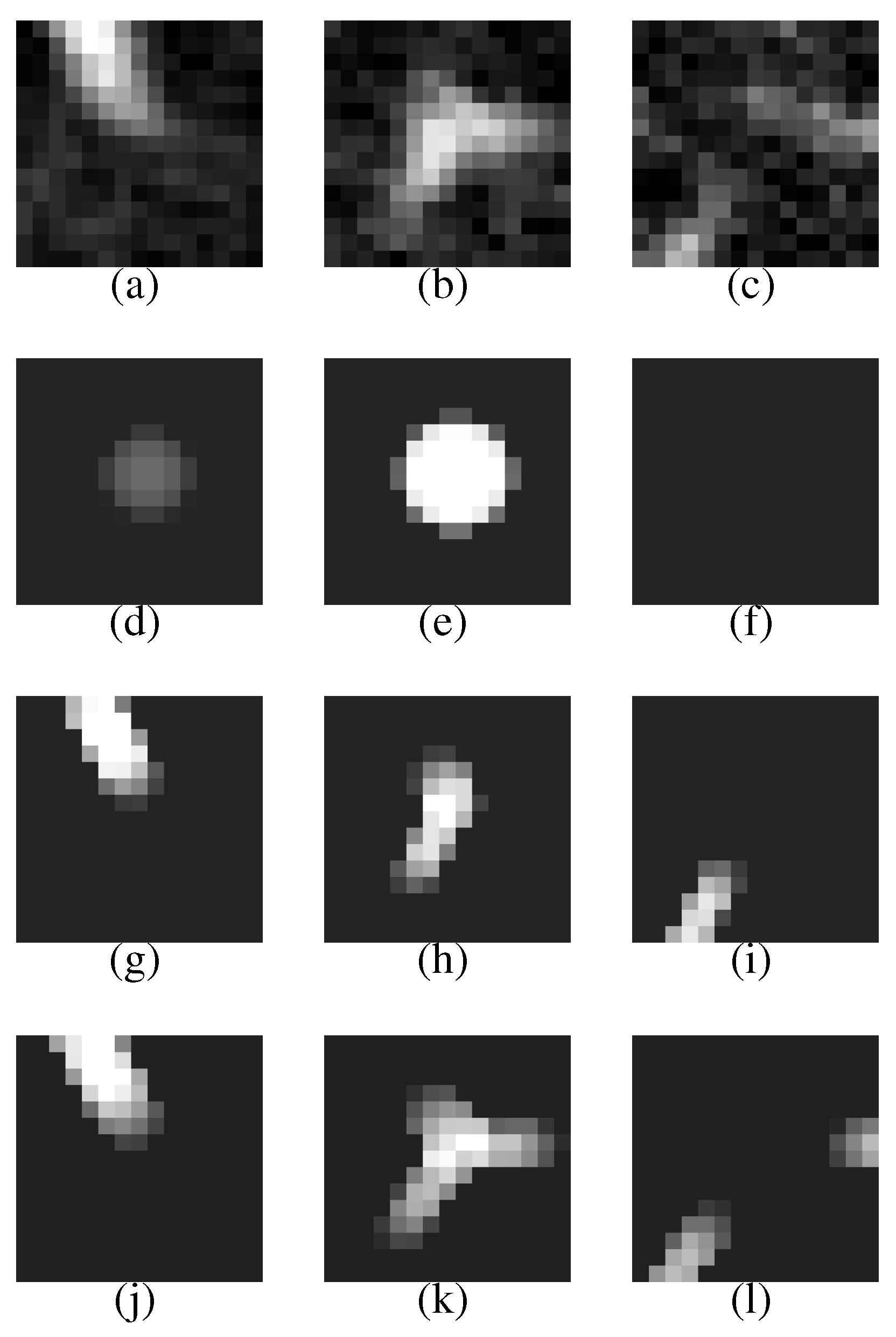
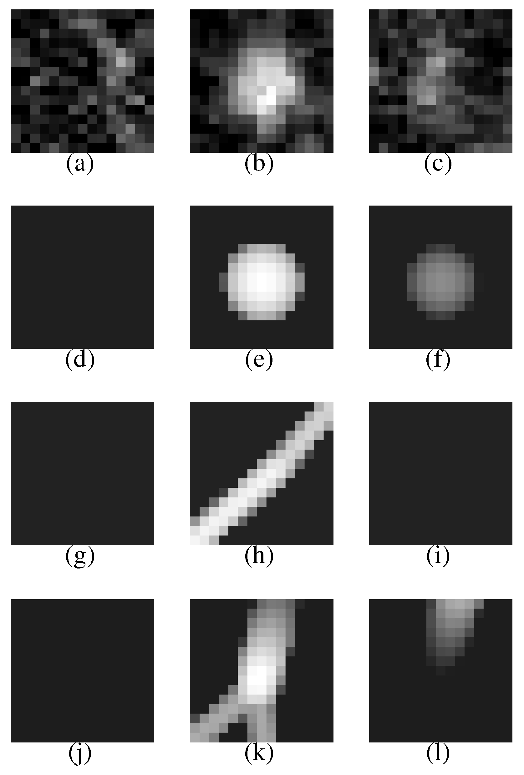
Figure 6 shows a slice cross section of a sample CT scan. The arrow indicates a nodule identified by a radiologist. The nodule is detected by our previous methods [8,27,28] as a nodule candidate. Figure 7 (a–c) shows a VOI of the nodule (Figure 7(b) shows the nodule). Figure 7(d–f) is template produced from the most likely nodule model that is depicted in Figure 8(a). They correspond to Figure 7(a–c), respectively. Figure 7(g–i) is produced from the most likely curved blood vessel model depicted in Figure 8(b), and Figure 7(j–l) is produced from the most likely bifurcated blood vessel model depicted in Figure 8(c). They correspond to Figure 7(a–c), respectively, in the same manner.

Figure 6. A slice cross section of a sample thoracic CT scan. The arrow indicates a nodule identified by a radiologist.

Figure 6. A slice cross section of a sample thoracic CT scan. The arrow indicates a nodule identified by a radiologist.

The posteriori probabilities of the most likely object models $o^N$, $o^{B_c}$ and $o^{B_b}$ are 0.124, 0.087 and 0.100, respectively (the common constant values are omitted), and the ratio of the posteriori probabilities ${\rho }_1$ is 1.24. Because the ratio is larger than the threshold $T_{\rho }$, the nodule candidate is correctly determined to be a nodule.

The nodule (Figure 7(a–c)) is faithfully reconstructed by the templates (Figure 7(d–f)). Although the nodule is shifted downward against the VOI (the nodule is not observed in the upper slice section shown in Figure 7(a)), the center of the nodule model is moved adequately. The nodule size is also estimated exactly. The diameters of the nodule and the nodule model are approximately 5.0 mm and 5.3 mm, respectively.

The effectiveness of Equation (3) can be seen in the templates of the curved and bifurcated blood vessel models shown in Figure 7(g–i) and (j–l), respectively. Because the nodule candidate is in the peripheral area of the lung region (see Figure 6 again), the mean radius of a blood vessel model ${\mu }_{r1}^B\left({\mathit{x}}^{B_c}\right)$ becomes rather small, 0.89 mm, at this position. The small mean radius produces thin regions on the templates and the thin regions make the correlation coefficients low. Therefore, the probabilities of the blood vessel models become smaller than that of the nodule model.

Figure 7. The first row represents the VOI comprising the nodule shown in Figure 6. The second, third and fourth rows represent the templates that are produced from the most likely nodule, curved blood vessel and bifurcated blood vessel models, respectively.

Figure 7. The first row represents the VOI comprising the nodule shown in Figure 6. The second, third and fourth rows represent the templates that are produced from the most likely nodule, curved blood vessel and bifurcated blood vessel models, respectively.

Figure 8. The most likely nodule, curved blood vessel and bifurcated blood vessel models for the nodule shown in Figure 6.

Figure 8. The most likely nodule, curved blood vessel and bifurcated blood vessel models for the nodule shown in Figure 6.

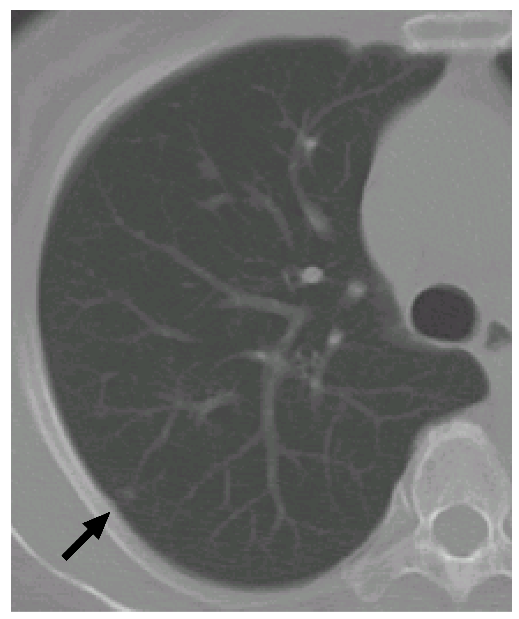
7.2. Case 2

Figure 9 shows another CT scan with a nodule. Figure 10 shows its VOI and templates, and Figure 11 the most likely object models. The posteriori probabilities are 0.121, 0.100 and 0.101, and the ratio is 1.20, that is larger than the threshold. Although the nodule is small (its diameter is approximately 3.8 mm), it is correctly determined to be a nodule.

Figure 9. The arrow indicates another nodule.

Figure 9. The arrow indicates another nodule.

Figure 10. A VOI of the nodule shown in Figure 9 and its templates.

Figure 10. A VOI of the nodule shown in Figure 9 and its templates.

Figure 11. The most likely object models for the nodule shown in Figure 9.

Figure 11. The most likely object models for the nodule shown in Figure 9.

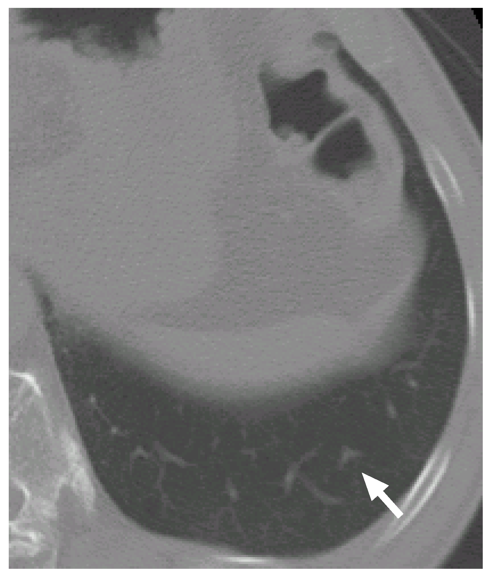
7.3. Case 3

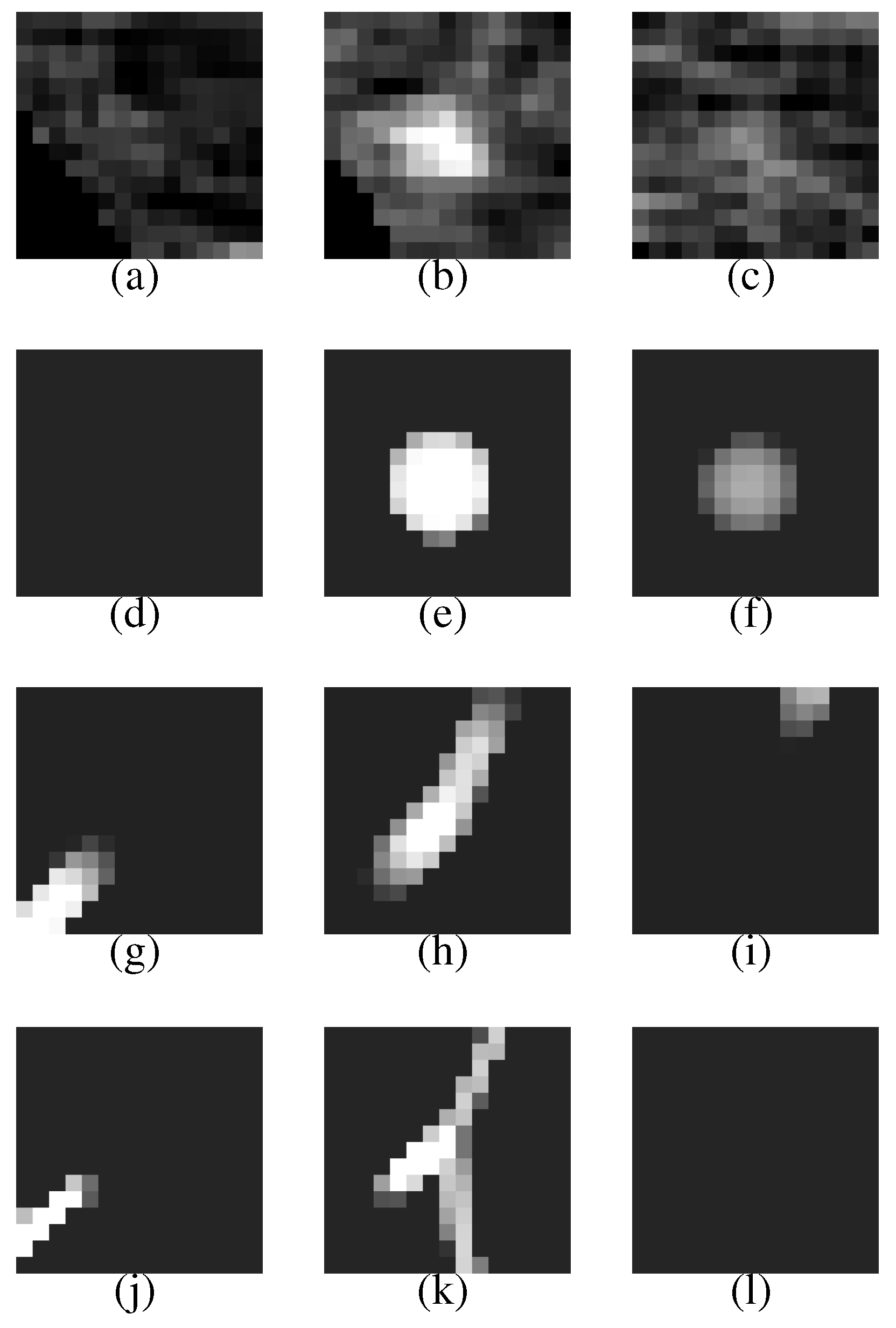
Figure 12 shows another CT scan with a false positive (a bifurcation in a blood vessel tree). Figure 13 shows its VOI and templates, and Figure 14 the most likely object models. The posteriori probabilities are 0.0960, 0.111 and 0.126, and the ratio is 0.762, that is smaller than the threshold. The candidate is correctly determined to be a blood vessel.

The candidate region observed in Figure 13(b) seems to be a nodule that has an irregular shape. It is difficult to recognize the candidate region only from the single slice section. However, by considering the relations between the candidate region and the other regions in the adjacent slice sections, it becomes to be easy to determine that the regions arise from a blood vessel bifurcation.

Figure 12. A bifurcation in a blood vessel tree.

Figure 12. A bifurcation in a blood vessel tree.

Figure 13. A VOI of the nodule candidate shown in Figure 12 and its templates.

Figure 13. A VOI of the nodule candidate shown in Figure 12 and its templates.

Figure 14. The most likely object models for the candidate shown in Figure 12.

Figure 14. The most likely object models for the candidate shown in Figure 12.

8. Discussion

Many detection methods based on template-matching techniques use only nodule templates [23,24,25]. Our method, on the other hand, uses not only the nodule templates but also blood vessel templates, that enable the computers to make the most of anatomical knowledge, especially, for blood vessel structures in lung regions. If the blood vessel models are not used in the present method and the nodule recognition is performed by

$${\rho }_2\left(v_C\right)=P\left(O^N(\Delta \Delta {\Omega }_N^N(l,n;{\omega }^{N*}))|v_C\right)$$

(25)

instead of Equation (24), the false positive number increases to 60.3 per case. It implies that the blood vessel models play an important role for nodule recognition.

The geometric averages of probabilities are also important. If the following probability ratio that consists of the ordinary joint probabilities is used:

$$\begin{array}{c}\hfill {\rho }_3\left(v_C\right)=\frac{p\left(o^N\left({\omega }^N\right)|v_C\right)}{{\displaystyle \underset{\tau \ne N}{max}p\left(o^{\tau }\left({\omega }^{\tau }\right)|v_C\right)}}\end{array}$$

(26)

the false positive number increases to 34.8 per case. The ordinary joint probabilities suppress all the priori probabilities of bifurcated blood vessel models as mentioned in Section 4, and therefore most bifurcated blood vessel models are ignored in the maximum operation in Equation (26) and the anatomical knowledge on bifurcated blood vessels is not made use of at all. It makes the recognition accuracy degraded.

The present method needs approximately 40 seconds for recognition of one candidate with a computer that has a 3 GHz CPU. We have already proposed an efficient template-matching method [35], but it uses simple object models that possess less parameters. A more efficient technique are needed for high-dimensional object models used in the present paper.

Our previous methods [8,27,28] are applied to CT scans for initial detection of nodule candidates as mentioned in Section 1 The method [8] is a Morphological [7] image filter that is designed to respond only to blob regions that are major shapes of pulmonary nodules on CT slice sections. The method [27] discriminates pulmonary nodules from false positives based on analysis of image features such as intensities, sizes and shapes. The method [28] recognizes nodules using a principal component analysis based clustering followed by a subspace method [36]. Although these methods use only 2-D image features and therefore yield many false positives, they can complete the recognition in a shorter time. From the practical point of view, we use these initial detection methods before applying the method proposed in the present paper.

9. Conclusions

The present paper described a novel recognition method of pulmonary nodules in thoracic CT scans by use of 3-D deformable nodule and blood vessel models. The anatomical validity of these object models and their fidelity to CT scans were evaluated in the framework of the Bayes theorem. The most likely object model that maximized the posteriori probability was obtained for each VOI comprising a nodule candidate. The VOI was determined to be abnormal if the most likely object model was a nodule model, and vice versa. The proposed method was applied to 26 actual CT scans. The 77.2% of false positives were reduced successfully.