Segment LLL Reduction of Lattice Bases Using Modular Arithmetic

Abstract

The algorithm of Lenstra, Lenstra, and Lovász (LLL) transforms a given integer lattice basis into a reduced basis. Storjohann improved the worst case complexity of LLL algorithms by a factor of $O\left(n\right)$ using modular arithmetic. Koy and Schnorr developed a segment-LLL basis reduction algorithm that generates lattice basis satisfying a weaker condition than the LLL reduced basis with $O\left(n\right)$ improvement than the LLL algorithm. In this paper we combine Storjohann’s modular arithmetic approach with the segment-LLL approach to further improve the worst case complexity of the segment-LLL algorithms by a factor of $n^{0.5}$.

1. Introduction

Given row vectors $b_1,\dots ,b_n\in {\mathbb{Z}}^d$ an integer lattice L (for short lattice) is defined as

$$L:=\left\{v\in {\mathbb{Z}}^d|v=\sum _{i=1}^n{z}_i{b}_i,z_i\in \mathbb{Z},b_i\in {\mathbb{Z}}^d\right\}$$

Several important theoretical and practical problems benefit from studying lattices. These include problems in geometry [1], cryptography [2], and integer programming [3]. An important problem, whose study dates back to 18th century, is the problem of finding i-th successive minimum of a lattice, $i=1,\dots ,n$. This problem involves finding the smallest number ${\lambda }_i$ (and possibly an associated lattice element) such that there are i linearly independent elements in L of length at most ${\lambda }_i$ [1, Chapter 8]. The shortest lattice vector problem is a special case of finding the shortest lattice vector only. This is a difficult problem to solve. For example, it is shown by Ajtai [4] that the problem of finding the shortest non-zero lattice vector under $l_2$ norm is NP-hard under randomized reduction [4]. Micciancio [5] showed that an α-approximate version of this problem (under randomized reduction) remains NP-hard for any $\alpha <\sqrt{2}$. The problem of finding the shortest lattice vector under $l_{\infty }$ norm is shown in the class NP-complete by van Emde Boas [6].

Knowing that finding the exact shortest lattice basis is difficult in the worst case, the problem of finding approximate successive minima is addressed by many researchers. In this context various notions of reduced bases have been proposed. In particular, notions of LLL-reduced, semi-reduced, Korkine-Zolotarev reduced, Block 2k reduced, semi block 2k reduced, and segment reduced bases are used by Lenstra, Lenstra, and Lovász [7], Schönhage [8], Kannan [9], Schnorr [10], and Koy and Schnorr [11], respectively. We define these and additional concepts below.

1.1. Definitions of Reduced Lattice Bases

Without loss of generality we assume that $b_1,\dots ,b_n$ are linearly independent. Superscript t is used to denote the transpose of a vector or a matrix. The $l_2$ norm is given by $\parallel y\parallel ={\left(y{y}^t\right)}^{0.5}$. $\left[x\right]$ denotes the nearest integer to a real number x (if non-unique then choose the candidate with smallest magnitude), $\lceil x\rceil$ denotes the smallest integer greater than or equal to x, and $\lfloor x\rfloor$ denotes the largest integer less than or equal to x. $T_{i,j}$ is the entry at the i-th row and j-th column of a matrix T. We use I to represent an identity matrix, and $e_i$ to represent its i-th column.

Let $B\in {\mathbb{Z}}^{n\times d}$ be such that the i-th row of B is given by $b_i$ for $1\le i\le n$. For a given lattice basis $b_1,\dots ,b_n$ the Gram-Schmidt algorithm determines the associated orthogonal vectors $b_1^{*},\dots ,b_n^{*}$ together with coefficients ${\Gamma }_{j,i}(1\le j<i\le n)$ defined inductively by

$$b_i^{*}=b_i-\sum _{j=1}^{i-1}{\Gamma }_{j,i}{b}_j^{*},\text{where}{\Gamma }_{j,i}=b_j^{*}{b}_i^t/{\parallel b_j^{*}\parallel }^2$$

(1.1)

This can be rewritten as $B={\Gamma }^t{B}^{*}$, where $B^{*}$ denotes the matrix whose i-th row is $b_i^{*}$, and Γ is a upper triangular matrix with ${\Gamma }_{i,i}=1$ and ${\Gamma }_{j,i}$ ($j<i$) is given in (1.1). Let $D_{i,\dots ,j}:=\parallel b_i^{*}{\parallel }^2\cdots {\parallel b_j^{*}\parallel }^2$. We denote $D_{1,\dots ,l}$ by $d_l$. Note that $d_n$ is the Gramian determinant of B. When we are considering k segments of B and $B^{*}$, $D_{k(l-1)+1,\cdots ,kl}:=\parallel b_{k(l-1)+1}^{*}{\parallel }^2\cdots {\parallel b_{kl}^{*}\parallel }^2$ is the segment Gramian determinant, and for simplicity we denote it by $D\left(l\right)$, where k is fixed.

D1. 

A basis is called size-reduced if $|{\Gamma }_{j,i}|\le 1/2for1\le j<i\le n.$ The notion of a size reduced basis goes back to Hermite [12].

D2. 

A basis is called (δ,η)-reduced if $(\delta -{\Gamma }_{i,i+1}^2)\parallel b_i^{*}{\parallel }^2\le {\parallel b_{i+1}^{*}\parallel }^2$ for $i=1,\dots ,n-1$, $\delta \in (\frac{1}{4},1]$, $|{\Gamma }_{j,i}|\le \eta$, $\eta \in [1/2,\sqrt{\delta })$. For $\delta =\frac{3}{4}$ and $|{\Gamma }_{j,i}|\le 1/2$ it is called 2-reduced because the above inequality becomes $\parallel b_i^{*}{\parallel }^2\le 2{\parallel b_{i+1}^{*}\parallel }^2$. A basis is called δ-LLL reduced if it is size-reduced and δ-reduced. It is simply called LLL reduced if it is size-reduced and 2-reduced. The LLL reduced basis was introduced by Lenstra, Lenstra, and Lovász [7].

D3. 

A basis is called semi-reduced if it is size-reduced and satisfies weaker conditions $\parallel b_i^{*}{\parallel }^2\le 2^n{\parallel b_{i+1}^{*}\parallel }^2$ for $i=1,\dots ,n-1$.

D4. 

A basis is called Korkine-Zolotarev basis if it is size-reduced and if $\parallel b_i^{*}\parallel ={\lambda }_1\left(L_i\right)$ for $i=1,\dots ,n,$ where $L_i$ is the orthogonal projection of L on the orthogonal complement of $span\{b_1,\dots ,b_{i-1}\}$.

The concepts of block reduced and segment reduced basis are defined by dividing a basis into k blocks or segments, i.e., $n=mk$, and then specifying appropriate conditions on basis vectors within each block and among blocks.

D5. 

A basis $b_1,\dots ,b_{mk}$ is called Block KZ reduced basis if it is size-reduced and if the projections of all $2k$-blocks $b_{ik+1},\dots ,b_{(i+2)k}$ on the orthogonal complement of $span\{b_1,\dots ,b_{ik}\}$ for $i=0,\dots ,m-2$ are Korkine-Zolotarev reduced.

D6. 

A basis $b_1,\dots ,b_{mk}$ is called k-segment LLL reduced if the following conditions hold.

C1.

It is size-reduced.

C2.

$(\delta -{\Gamma }_{i,i+1}^2)\parallel b_i^{*}{\parallel }^2\le {\parallel b_{i+1}^{*}\parallel }^2$ for $i\ne kl$, $l\in \mathbb{Z}$, i.e., vectors within each segment of the basis are δ-reduced, and

C3.

Letting $\alpha :=1/(\delta -\frac{1}{4})$, two successive segments of the basis are connected by the following two conditions.

C3.1.

$D\left(l\right)\le {(\alpha /\delta )}^{k^2}D(l+1)$for$l=1,\dots ,m-1$.

C3.2.

${\delta }^{k^2}\parallel b_{kl}^{*}{\parallel }^2\le \alpha {\parallel b_{kl+1}^{*}\parallel }^2$for$l=1,\dots ,m-1$.

The case where $k=O\left(\sqrt{n}\right)$ is of special interest.

1.2. Discussion on Various Reduced Bases

The ratios $\frac{\parallel b_i{\parallel }^2}{{\lambda }_i^2},i=1,\dots ,n$ are used to measure the quality of various reduced bases defined above. We call these approximation ratios. Known bounds on approximation ratios for various reduced bases, known algorithms for generating them, the worst case running time of these algorithms, and the bit-precision used in performing the computations (addition, subtraction, multiplication and division) in these algorithms are summarized in Table 1. The bounds in this table assume $k=O\left(\sqrt{n}\right)$, and $d=O\left(n\right)$. Following [7,8] we use $M_{sc}:=max\{2^n,M_0,d_1,\dots ,d_n\}$, where $M_0:={max}_{i=1,\dots ,n}{\parallel b_i\parallel }^2$ to measure the complexity of these algorithms. Note that $M_{sc}=2^{O\left(n^2\right)}$ when $\parallel b_i\parallel =2^{O\left(n\right)}$.

The work of Lenstra, Lenstra, and Lovász [7] is seminal on finding a reduced lattice basis, and its implication on the problem of finding successive minima. Their algorithm for finding an LLL reduced basis is polynomial time. In particular, for $M_{sc}=2^{O\left(n^2\right)}$ in the worst case it requires $O\left(n^5\right)$ arithmetic operations using $O\left(n^2\right)$ bit numbers. Since the development of the LLL algorithm significant effort has been directed towards developing methods for finding an improved quality basis in polynomial time, and finding a worse quality basis with a better worst case computational complexity. Research has also progressed towards generalizing the LLL algorithm to arbitrary norms [18,19].

Table 1. Summary of various LLL-related Algorithms.

Algorithm	Lower Bounds on $\frac{\parallel b_i{\parallel }^2}{{\lambda }_i^2}$	Upper Bounds on $\frac{\parallel b_i{\parallel }^2}{{\lambda }_i^2}$	Arithmetic Steps	Precision
LLL reduced [7]	${\alpha }^{1-i}{\delta }^n$	${\alpha }^{n-1}{\delta }^{-n}$	$O\left(n^3{log}_{1/\delta }{M}_{sc}\right)$	$O(ln{M}_{sc})$
LLL reduced [13]	${\alpha }^{1-i}{\delta }^n$	${\alpha }^{n-1}{\delta }^{-n}$	$O\left(n^3{log}_{1/\delta }{M}_{sc}\right)$	$O(n+ln{M}_0)$
Modular LLL [14]	${\alpha }^{1-i}{\delta }^n$	${\alpha }^{n-1}{\delta }^{-n}$	$O\left(n^2{log}_{1/\delta }{M}_{sc}\right)$	$O(ln{M}_{sc})$
Semi-reduced [8]	${\alpha }^{1-i-2n}$	${\alpha }^{2n-1}$	$O\left(n^2{log}_{1/\delta }{M}_{sc}\right)$	$O(ln{M}_{sc})$
Kannan [9]	$\frac{4}{i+3}$	$\frac{i+3}{4}$	$n^{O\left(n\right)}ln{M}_0$	$O(n^{2}ln{M}_0)$
Block KZ [10,15] 1	$\frac{4}{i+3}{\gamma }_{2k}^{-2\frac{i-1}{2k-1}}$	${\gamma }_{2k}^{2\frac{n-i}{2k-1}}\frac{i+3}{4}$	$O(n^{(\sqrt{n}/2+o\left(\sqrt{n}\right))}+n^{4}ln{M}_0)$	$O(nln{M}_0)$
Segment LLL [11]	${\alpha }^{1-i}{\delta }^{3n}$	${\alpha }^{n-1}{\delta }^{-3n}$	$O\left(n^2{log}_{1/\delta }{M}_{sc}\right)$	$O(ln{M}_{sc})$
Mod-Seg LLL	${\alpha }^{1-i}{\delta }^{3n}$	${\alpha }^{n-1}{\delta }^{-3n}$	$O\left(n^{1.5}{log}_{1/\delta }{M}_{sc}\right)$	$O(ln{M}_{sc})$
Mod-Seg LLL FMM	${\alpha }^{1-i}{\delta }^{3n}$	${\alpha }^{n-1}{\delta }^{-3n}$	$O\left(n^{1.382}{log}_{1/\delta }{M}_{sc}\right)$	$O(ln{M}_{sc})$
Nguyen and Stehle [16] $L^2$	${\alpha }^{1-i}{\delta }^n$	${\alpha }^{1-i}{\delta }^{-n}$	$O\left(n^2(n+ln\left(M_0\right)){ln}_{1/\delta }\left(M_{sc}\right)\right)$	$1.58n$ fl
Schnorr [17] SLL	${\alpha }^{1-i}{\delta }^{7n}$	${\alpha }^{n-1}{\delta }^{-7n}$	$O(n^{2}lnn{log}_{1/\delta }{M}_{sc})$	$3n+d$ fl

¹ ${\gamma }_n$ is the Hermite constant which is defined as ${\gamma }_n=\text{sup}\{{\lambda }_1{(L)}^2{d}_n^{-\frac{1}{n}}:\text{for lattices }L\text{ of rank }n\}$.

Table 1. Summary of various LLL-related Algorithms.

Algorithm	Lower Bounds on $\frac{\parallel b_i{\parallel }^2}{{\lambda }_i^2}$	Upper Bounds on $\frac{\parallel b_i{\parallel }^2}{{\lambda }_i^2}$	Arithmetic Steps	Precision
LLL reduced [7]	${\alpha }^{1-i}{\delta }^n$	${\alpha }^{n-1}{\delta }^{-n}$	$O\left(n^3{log}_{1/\delta }{M}_{sc}\right)$	$O(ln{M}_{sc})$
LLL reduced [13]	${\alpha }^{1-i}{\delta }^n$	${\alpha }^{n-1}{\delta }^{-n}$	$O\left(n^3{log}_{1/\delta }{M}_{sc}\right)$	$O(n+ln{M}_0)$
Modular LLL [14]	${\alpha }^{1-i}{\delta }^n$	${\alpha }^{n-1}{\delta }^{-n}$	$O\left(n^2{log}_{1/\delta }{M}_{sc}\right)$	$O(ln{M}_{sc})$
Semi-reduced [8]	${\alpha }^{1-i-2n}$	${\alpha }^{2n-1}$	$O\left(n^2{log}_{1/\delta }{M}_{sc}\right)$	$O(ln{M}_{sc})$
Kannan [9]	$\frac{4}{i+3}$	$\frac{i+3}{4}$	$n^{O\left(n\right)}ln{M}_0$	$O(n^{2}ln{M}_0)$
Block KZ [10,15] 1	$\frac{4}{i+3}{\gamma }_{2k}^{-2\frac{i-1}{2k-1}}$	${\gamma }_{2k}^{2\frac{n-i}{2k-1}}\frac{i+3}{4}$	$O(n^{(\sqrt{n}/2+o\left(\sqrt{n}\right))}+n^{4}ln{M}_0)$	$O(nln{M}_0)$
Segment LLL [11]	${\alpha }^{1-i}{\delta }^{3n}$	${\alpha }^{n-1}{\delta }^{-3n}$	$O\left(n^2{log}_{1/\delta }{M}_{sc}\right)$	$O(ln{M}_{sc})$
Mod-Seg LLL	${\alpha }^{1-i}{\delta }^{3n}$	${\alpha }^{n-1}{\delta }^{-3n}$	$O\left(n^{1.5}{log}_{1/\delta }{M}_{sc}\right)$	$O(ln{M}_{sc})$
Mod-Seg LLL FMM	${\alpha }^{1-i}{\delta }^{3n}$	${\alpha }^{n-1}{\delta }^{-3n}$	$O\left(n^{1.382}{log}_{1/\delta }{M}_{sc}\right)$	$O(ln{M}_{sc})$
Nguyen and Stehle [16] $L^2$	${\alpha }^{1-i}{\delta }^n$	${\alpha }^{1-i}{\delta }^{-n}$	$O\left(n^2(n+ln\left(M_0\right)){ln}_{1/\delta }\left(M_{sc}\right)\right)$	$1.58n$ fl
Schnorr [17] SLL	${\alpha }^{1-i}{\delta }^{7n}$	${\alpha }^{n-1}{\delta }^{-7n}$	$O(n^{2}lnn{log}_{1/\delta }{M}_{sc})$	$3n+d$ fl

¹ ${\gamma }_n$ is the Hermite constant which is defined as ${\gamma }_n=\text{sup}\{{\lambda }_1{(L)}^2{d}_n^{-\frac{1}{n}}:\text{for lattices }L\text{ of rank }n\}$.

The algorithm by Schönhage [8] finds a semi-reduced basis. It requires $O\left(n\right)$ less time over the LLL algorithm. However, the bounds on the approximation ratios for a semi-reduced basis are of a significantly lower quality. A better complexity for finding a semi-reduced basis is also proved by Storjohann [14].

Kannan [9] proposes an algorithm for finding Korkine-Zolotarev (KZ) basis that runs in $O(n^{O\left(n\right)}ln{M}_0)$ arithmetic operations on $O(n^{2}ln{M}_0)$ bit integers. Kannan’s algorithm uses the LLL algorithm as a black box. This bound for finding a KZ basis is improved by Schnorr [10] to $O(n^{n/2+o\left(n\right)}+n^{4}ln{M}_0)$ arithmetic operations using $O(nln{M}_0)$ bit integers. The bound for Schnorr’s algorithm in Table 1 is given for performing a KZ reduction of a block of size $2k$. Schnorr [10] further introduces the notion of a semi block 2k reduced basis, and uses this concept to show that a $O\left(k^{(n/k)}\right)$-approximate shortest vector is found in $O(n^2(k^{k/2+o\left(k\right)}+n^2)ln\left(M_0\right))$ arithmetic operation using $O(nln{M}_0)$ bit integers. This leads to a hierarchy of algorithms for finding the shortest lattice vector, and a semi block 2k reduced basis. The complexity in Table 1 is a special case where $k=\lfloor 2\sqrt{n}\rfloor$.

Koy and Schnorr [20] propose the concept of a segment reduced basis, and give an algorithm for finding such a basis. Similar to the semi-reduction algorithm of Schönhage [8] the segment reduction algorithm works with a subset of vectors in the lattice basis at a time. However, it worsens the approximation ratios only slightly, and in a controllable fashion. Moreover, it also achieves an $O\left(n\right)$ reduction in the worst case complexity over the LLL algorithm. Since the writing of the original draft of this paper improvements in computational complexity of the LLL and segment LLL algorithms have also been achieved by showing that the methods can be modified to perform computations using $O\left(n\right)$ bit floating point numbers. In particular, Nguyen and Stehle [16] rearranged computations in the Cholesky factorization algorithm and used Babai’s nearest point algorithm to update the Cholesky factor coefficients to show that the LLL-algorithm can be correctly implemented with $O\left(n\right)$ bit floating point precision computations. By making use of results from numerical analysis on Householder transformation using floating point arithmetic and rearrangement of computations in Gram-Schmidt algorithm Schnorr [17] has given an improved segment reduction algorithm that performs $O\left(n^{5+ϵ}\right)$ bit operations for input bases of length $2^{O\left(n\right)}$.

1.3. Paper Contribution and Organization

In this paper we show that the modular arithmetic computation approach of [14] can be combined with the segment concept in [20] to develop a modular segment reduction algorithm. The novelty of Storjohann’s is in rearranging the computations in LLL and delaying certain updates, which result in a computational savings by a factor of $O\left(n\right)$. The savings of $O\left(n\right)$ in [20] result from localizing the updates. We show that by combining the strength of the modular arithmetic approach with the Segment LLL algorithm an $O\left(n^{0.5}\right)$ further saving is possible in the worst case when initial integer basis vectors have $2^{O\left(n\right)}$ magnitude and $d=O\left(n\right)$. We also show that it is possible to further improve this complexity by using fast matrix multiplication.

This paper is organized as follows. In the next section we review the LLL basis reduction algorithm of Lenstra, Lenstra, and Lovász [7]. In addition we explain the basic computational observations of Storjohann in this section. In Section 3 we give Storjohann’s modular LLL reduction algorithm and give the essential results from [14]. Additional notation and concepts needed to describe the modular approach are also given in this section. In Section 4 we give the segment basis reduction algorithm. In Section 5 we describe the modular segment reduction algorithm proposed in this paper, and give its worst case complexity result.

2. Methods for LLL-Reduced Lattice Bases

2.1. The LLL Basis Reduction Algorithm

The LLL algorithm performs two essential computational steps. These are: (i) Size reduction of B by ensuring that $|{\Gamma }_{j,i}|\le 1/2$, $1\le j<i\le n$; (ii) swap of two adjacent rows of B, and subsequent restoration of Γ. We now explain these two steps.

Size Reduction of B

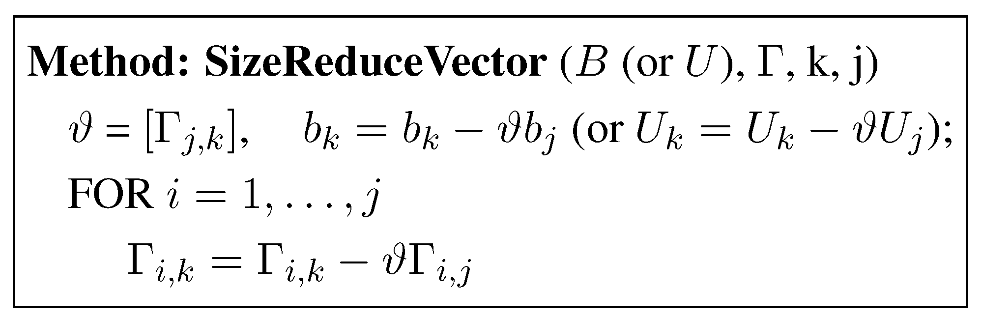
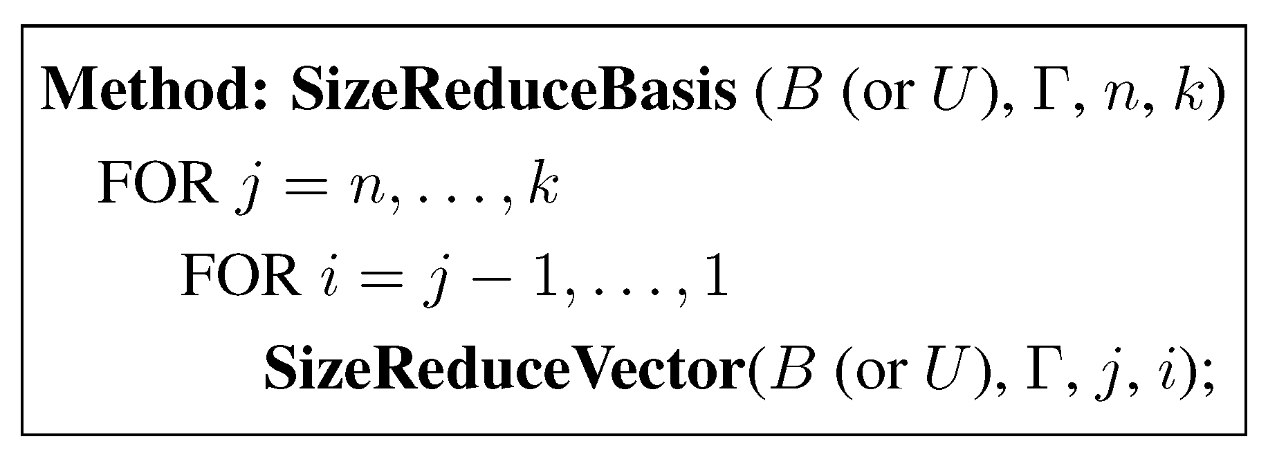
Let [${\widehat{b}}_1,\dots ,{\widehat{b}}_n$]=[$b_1,\dots ,b_{k-1},b_k-\left[{\Gamma }_{j,k}\right]b_j,\dots ,b_n]$ ($j<k$) be a basis obtained from $b_1,\dots ,b_n$. It can be rewritten as $\widehat{B}=U(j,k)B$, where $U(j,k)=I-\left[{\Gamma }_{j,k}\right]e_k{e}_j^T$ is an elementary unimodular matrix. It is easy to see that $\widehat{B}={\widehat{\Gamma }}^t{B}^{*}$, where $\widehat{\Gamma }=\Gamma -\left[{\Gamma }_{j,k}\right]\Gamma e_j{e}_k^T$. Note that $B^{*}$ is unchanged as a result of this operation. The operation results in $|{\widehat{\Gamma }}_{j,k}|\le 1/2$. This computation is called the size reduction of $b_k$ against $b_j$, $j<k$. Note that $\widehat{\Gamma }$ is obtained from Γ (i.e., Γ is updated) in $O\left(n\right)$ arithmetic operations. After initial Γ is computed, we can size reduce the entire basis by recursively applying this step in the order $(k,j)=(n,n-1),(n,n-2),\dots ,(n,1),(n-1,n-2),\dots ,(2,1)$. This is summarized in the methods SizeReduceVector and SizeReduceBasis. The method SizeReduceBasis is presented in a more general setting to allow for size reduction of limited number of vectors in B. Also, note that B need not be updated since all the information required to reduce B is contained in Γ. The update of B can be stored in a sequence of elementary unimodular matrices or their product. We represent this matrix by U.

Figure 1. Size Reduction of a Basis Vector.

Figure 1. Size Reduction of a Basis Vector.

Figure 2. Size Reduction of a Basis.

Figure 2. Size Reduction of a Basis.

Swap of Two Adjacent Rows of B

Let [${\widehat{b}}_1,\dots ,{\widehat{b}}_n$] = [$b_1,\dots ,b_k,b_{k-1},\dots ,b_n$] be a basis obtained from $b_1,\dots ,b_n$. It can be rewritten as $\widehat{B}=U(k-1,k)B$, where $U(k-1,k)$ is a permutation matrix that permutes the $(k-1)$-th row with the k-th row of B. This operation requires updating $\parallel b_{k-1}^{*}{\parallel }^2$ and $\parallel b_k^{*}{\parallel }^2$ of $B^{*}$ and the coefficients of column/row $k-1$ and k of Γ. This can be done by the following recurrence using $\mu :={\Gamma }_{k-1,k}$, $\nu :=\parallel b_k^{*}{\parallel }^2+{\mu }^2{\parallel b_{k-1}^{*}\parallel }^2$:

$$\begin{array}{ccc}& & {\Gamma }_{k-1,k}=\mu \parallel b_{k-1}^{*}{\parallel }^2/\nu ,\parallel b_k^{*}{\parallel }^2=\parallel b_{k-1}^{*}{\parallel }^2\parallel b_k^{*}{\parallel }^2/\nu ,{\parallel b_{k-1}^{*}\parallel }^2=\nu ,\hfill \end{array}$$

(2.2)

$$\begin{array}{ccc}& & \left[\begin{array}{c}{\Gamma }_{j,k-1}\hfill \\ {\Gamma }_{j,k}\hfill \end{array}\right]=\left[\begin{array}{c}{\Gamma }_{j,k}\hfill \\ {\Gamma }_{j,k-1}\hfill \end{array}\right]\text{for }j=1,\dots ,k-2,\hfill \end{array}$$

(2.3)

$$\begin{array}{ccc}& & \left[\begin{array}{c}{\Gamma }_{k-1,j}\hfill \\ {\Gamma }_{k,j}\hfill \end{array}\right]=\left[\begin{array}{cc}1\hfill & {\Gamma }_{k-1,k}\hfill \\ 0\hfill & 1\hfill \end{array}\right]\left[\begin{array}{cc}0& 1\\ 1& -\mu \end{array}\right]\left[\begin{array}{c}{\Gamma }_{k-1,j}\hfill \\ {\Gamma }_{k,j}\hfill \end{array}\right],\text{for }j=k+1,\dots ,n.\hfill \end{array}$$

(2.4)

We refer to the procedure implementing above recurrence by Swap (B (or U),$\Gamma ,k,k-1\left)\right)$.

The absolute value of the coefficients in the $(k-1)$-th and k-th rows of Γ obtained after the swap can become larger than $1/2$, a further size reduction step is performed to ensure that these coefficients are less than $1/2$. Note that while the restoration of Γ resulting from swap requires $O\left(n\right)$ arithmetic operations, the size reduction step requires $O\left(n^2\right)$ operations. Hence, the worst case effort resulting from a swap of two adjacent rows is $O\left(n^2\right)$.

The Lenstra, Lenstra, and Lovász [7] algorithm for finding an LLL-reduced basis is summarized in Figure 3. The number of swaps and the effort needed to restore the size reduced property of B determines the worst case complexity of the LLL algorithm.

Lenstra, Lenstra, and Lovász [7] maintain size reduced property of B for two reasons. The first reason is in checking the condition in the IF statement of the LLL algorithm. This allows us to produce an LLL-reduced basis upon the termination of their algorithm. Second, the size reduced property of B is used to bound the size of intermidate numbers generated in the algorithm, which is necessary to establish polynomial time complexity of the algorithm.

Figure 3. The LLL Basis Reduction Algorithm.

Figure 3. The LLL Basis Reduction Algorithm.

Figure 4 rearranges the computations in the LLL algorithm of Figure 3 without changing the algorithm. For the moment we are not concerned with the issue of the size of intermediate numbers. In particular, the algorithm in Figure 4 will produce the same basis as the algorithm in Figure 3. In fact, if the computations are performed in infinite precision, then the step indicated in ♠ is not even necessary. If this step is deleted, then the cost of the restoration of Γ after each swap reduces from $O\left(n^2\right)$ to $O\left(n\right)$ arithmetic operations. Storjohann [14] achieves this while maintaining finite precision with computation on integers of appropriate length by using modular arithmetic.

Figure 4. The LLL Basis Reduction Algorithm with Rearranged Computations.

Figure 4. The LLL Basis Reduction Algorithm with Rearranged Computations.

3. Storjohann’s Improvements

We now describe Storjohann’s [14] modifications. The LLL algorithm is first described as a fraction free algorithm to allow all computations on integer (not rational) numbers. The modular arithmetic modification that allows one to maintain finite precision is given subsequently.

3.1. The LLL-Reduction with Fraction Free Computations

For the matrix $B{B}^t$ we have an integral lower triangular matrix F and an integral upper triangular matrix T such that $T=F\left(B{B}^t\right)$ (See Geddes, Czapor, and Labahn [21]). F and T are called the fraction free factors of $B{B}^t$. Fraction free factors of a matrix are computed in $O\left(n^3\right)$ arithmetic operations using standard matrix multiplication. It is known that

$$\begin{array}{c}\hfill T=F\left(B{B}^t\right)=\left[\begin{array}{cccc}{d}_1& \dots & \dots & \dots \\ & \ddots & T_{i,j}& ⋮\\ & & \ddots & ⋮\\ & & & d_n\end{array}\right]\end{array}$$

(3.5)

where $T_{i,j}=d_j{\Gamma }_{i,j}$. Recall that $B{B}^t$ is positive definite since the row vectors of B are linearly independent. Hence T and F are unique. Also, $F=diag\{1,d_1,\dots ,d_{n-1}\}{\Gamma }^{-t}$, $T=diag\{d_1,\dots ,d_n\}\Gamma$, $\parallel b_i^{*}{\parallel }^2=d_i/d_{i-1}$ while taking $d_0=1$, and $d_1,\dots ,d_n$ are integers because $b_1,\dots ,b_n$ are in ${\mathbb{Z}}^d$. Note also that $T{F}^t=diag\{d_1,d_1{d}_2,d_2{d}_3,\dots ,d_{n-1}{d}_n\}$.

Storjohann [14] gave a fast matrix multiplication algorithm for computing F and T. It requires $O(n^{\theta }ln\left(n\right){(ln{M}_{sc})}^{1+ϵ})$ bit operations on integers of bit length $O(ln{M}_{sc})$, where $\theta <2.376$ and ϵ is a positive constant when the fast matrix multiplication algorithm of Coppersmith and Winograd [22] is used. $\theta =3$ and $ϵ=1$ when the standard matrix multiplication is used.

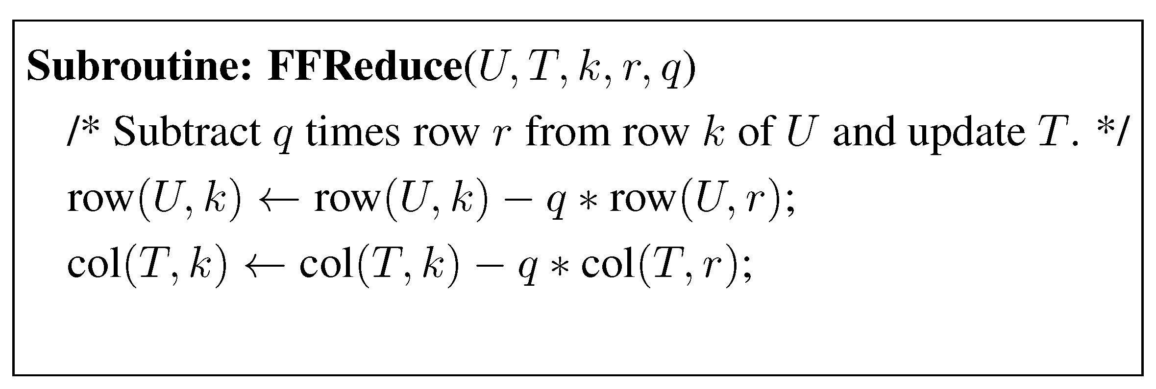
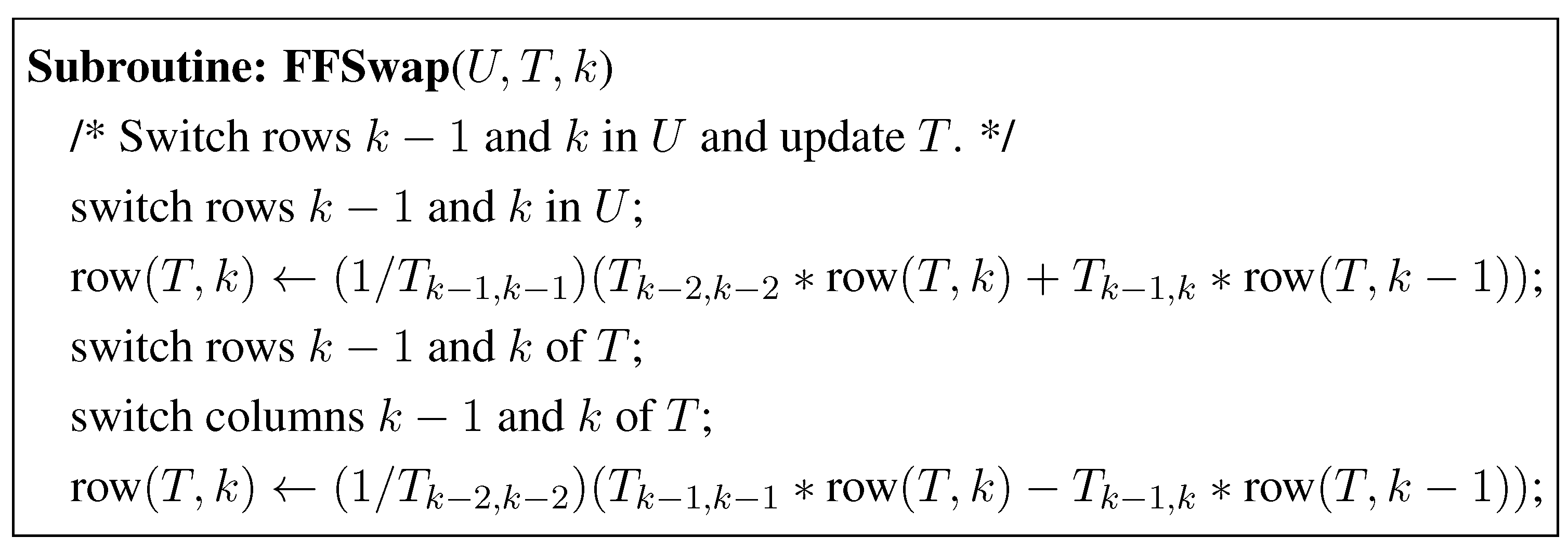
In Figure 5 we give Storjohann’s rearrangement of the computations of Figure 4 using fraction free computation. The ModifiedLLL algorithm performs two types of unimodular operations. (i) FFReduce: subtracting a multiple of a row of B from another row of B, and (ii) FFSwap: swapping a row of B with an adjacent row of B. The ModifiedLLL algorithm works by recording the unimodular row operations on B in a unimodular matrix U initially set to be an identity matrix, and updating the entries of T. There is no need to update B or $B^{*}$ in the algorithm, except in a post processing step. It is sufficient to update matrices U and T during the algorithm’s iterations. The fraction free updates of U and T corresponding to these unimodular operations are given in Figure 6 and Figure 7, respectively. Note that one execution of FFReduce or FFSwap is performed in $O\left(n\right)$ arithmetic operations.

Figure 5. Modified LLL Basis Reduction Algorithm.

Figure 5. Modified LLL Basis Reduction Algorithm.

Figure 6. Fraction Free Subtract Subroutine.

Figure 6. Fraction Free Subtract Subroutine.

Figure 7. Fraction Free Swap Subroutine.

Figure 7. Fraction Free Swap Subroutine.

The LLL and ModifiedLLL algorithms use $\Delta :={\prod }_{i=1}^{n-1}{d}_i$ to measure progress. The FFSwap step of the algorithm reduces Δ by a factor δ [7]. This is because when $b_k$ and $b_{k-1}$ are swapped, $\parallel b_{k-1}^{*}{\parallel }^2{\parallel b_k^{*}\parallel }^2$ remains constant, and the new value of $\parallel b_{k-1}^{*}{\parallel }^2$ is reduced at least by a factor δ. As a consequence $d_{k-1}$ is reduced by a factor δ, while all other $d_i$ do not change. The value of Δ is unchanged in the FFReduce step of the algorithm because $B^{*}$ does not change after this step. Since $1\le \Delta \le M_{sc}^{n-1}$, Case 1 in the ModifiedLLL algorithm occurs only $O\left(n{log}_{1/\delta }{M}_{sc}\right)$ times. Hence this part of the algorithm is executed in $O\left(n^2{log}_{1/\delta }{M}_{sc}\right)$ arithmetic operations. Case 2 of the algorithm can also occur at most $O\left(n{log}_{1/\delta }{M}_{sc}\right)$ times, each requiring $O\left(n^2\right)$ arithmetic operations. Hence, this part of the algorithm is executed in $O\left(n^3{log}_{1/\delta }{M}_{sc}\right)$ arithmetic operations. Finally a δ-LLL reduced basis is generated by $UB$, which is performed in $O\left(n^{2}d\right)$ operations under standard matrix multiplication, and in $O\left(n^{1.376}d\right)$ using the algorithm of Coppersmith and Winograd [14,22]. Lenstra, Lenstra, and Lovász [7] showed that the bit length of the numbers on which the arithmetic operations are performed is bounded by $O\left({log}_2{M}_{sc}\right)$. This gives the complexity result in Table 1, where $d=O\left(n\right)$ for simplicity.

The following lemma gives bounds on the size of intermediate lattice bases generated during the LLL and ModifiedLLL algorithms. This property is used when using computations with modular arithmetic.

Lemma 1 

[7]. Let B be an input basis to the LLL and ModifiedLLL algorithms. The quantities ${max}_i\{\parallel b_i^{*}\parallel \}$ and ${max}_i\left\{d_i\right\}$ are non-increasing in the LLL and ModifiedLLL algorithms. Furthermore, upon termination

$$\parallel b_i{\parallel }^2\le n{M}_0,\text{for}1\le i\le n$$

Proof: 

Recall that size reduction/subtract does not change $B^{*}$, consequently for all i, $\parallel b_i^{*}\parallel$ is unchanged in this step. Swapping $b_i$ and $b_{i-1}$ decreases $\parallel b_{i-1}^{*}\parallel$ by a factor of δ and the updated $\parallel b_i^{*}\parallel$ is bounded by old $\parallel b_{i-1}^{*}\parallel$. Hence, the non-increasing property is established. We have $\parallel b_i{\parallel }^2=\parallel b_i^{*}{\parallel }^2+{\sum }_{j=1}^{i-1}{\Gamma }_{j,i}^2{\parallel b_j^{*}\parallel }^2\le n{M}_0$, since $\parallel b_i^{*}\parallel \le \parallel b_i\parallel \le M_0$ in the beginning, and throughout the LLL and ModifiedLLL algorithms. The bounds obviously hold at termination. ☐

3.2. The Modified LLL Algorithm with Modular Arithmetic

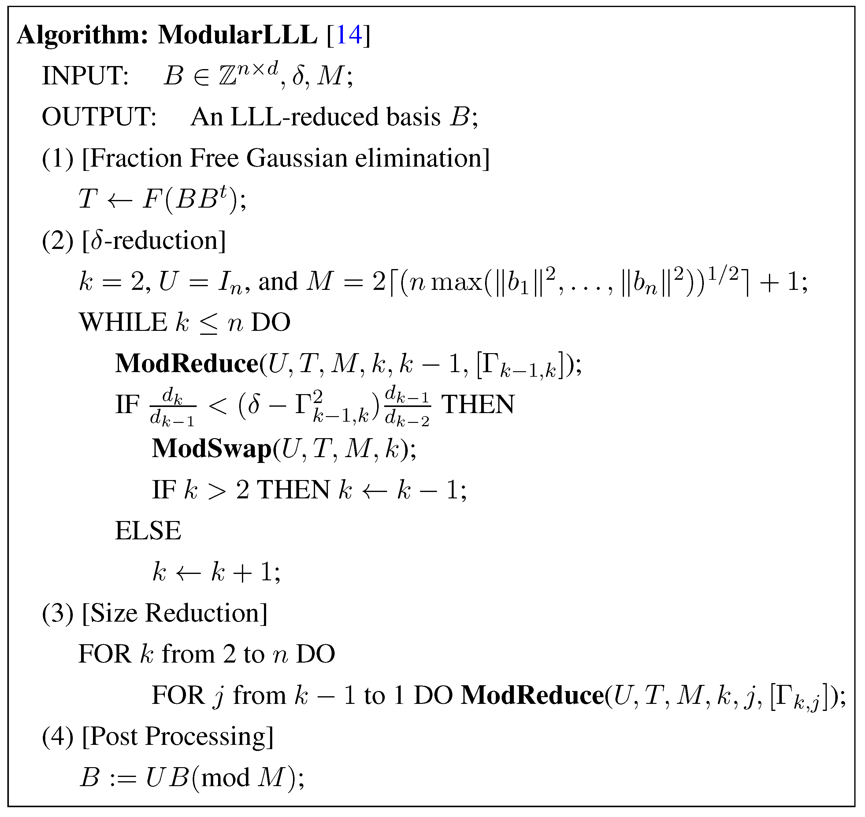
Storjohann [14] uses modular arithmetic to keep the intermediate numbers bounded during the algorithm’s iterations. Given an integer a, and an integer $M>0$, we write $a\left(modM\right)$ to mean the unique integer r congruent to a modulo M in the symmetric range, that is, with $-\lfloor (M-1)/2\rfloor \le r\le \lfloor M/2\rfloor$. Similarly, $U\left(modM\right)$ stands for the same operation for all entries of matrix U.

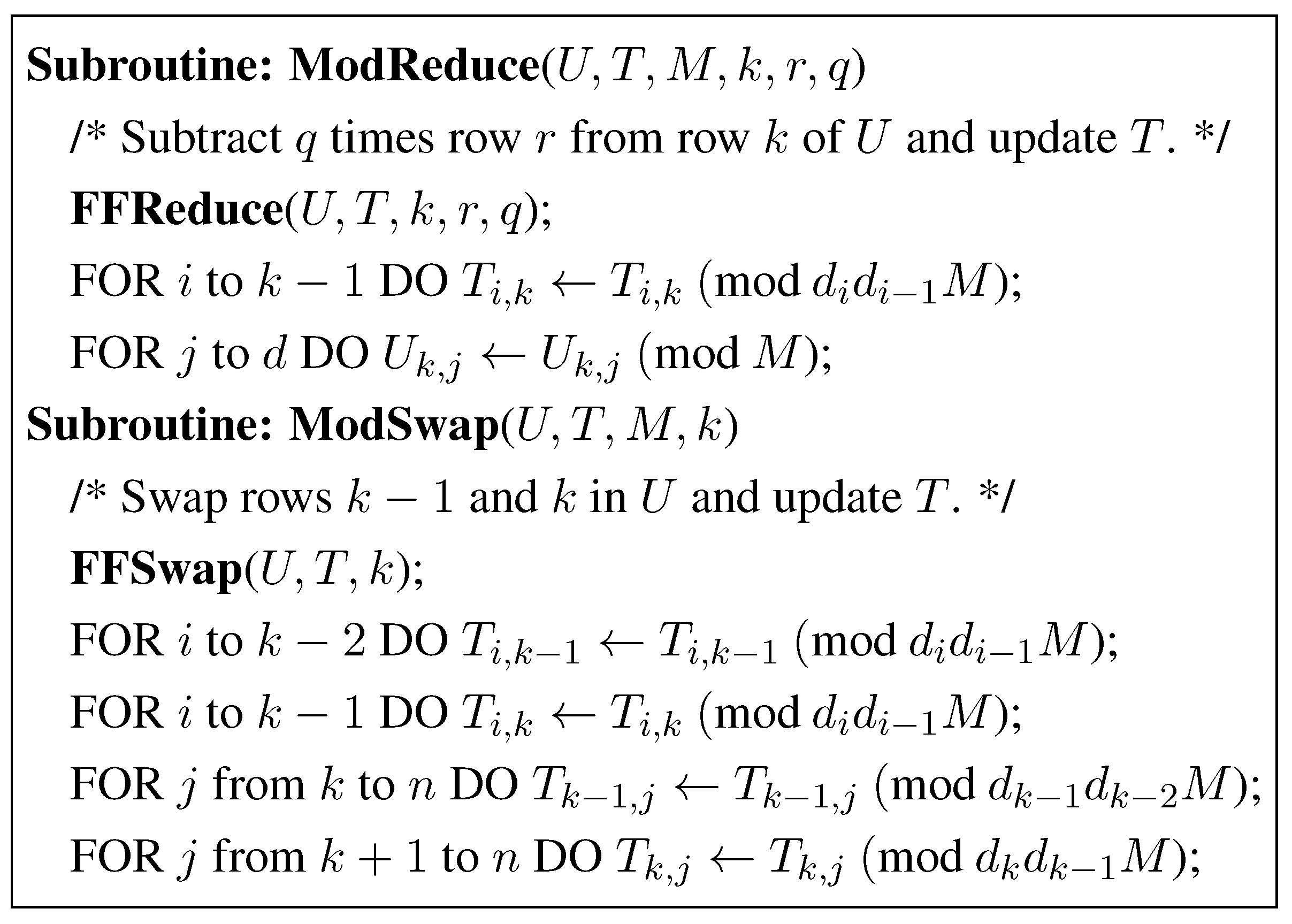
The modular basis reduction algorithm of Storjohann [14] is given in Figure 8 and Figure 9. Its worst case computational complexity is given in Table 1. The notable difference of this algorithm from the ModifiedLLL algorithm is in the modular arithmetic operation that is performed in the methods ModReduce and ModSwap.

Let $M=2\lceil {\left(n{M}_0\right)}^{1/2}\rceil +1$ so that by Lemma 1 the entries in the reduced basis matrix upon the termination of the ModifiedLLL algorithm are bounded in magnitude by $(M-1)/2$. The modular approach hinges on the observation that $UB\left(modM\right)=\overline{U}B\left(modM\right)$, where $\overline{U}=U\left(modM\right)$. Note that in the “infinite" precision version of the $\mathbf{Modified}\mathbf{LLL}$ algorithm, where the ♠ step is not performed, one allows U to grow. However, in the modular arithmetic version the elements of U and T remain bounded.

Figure 8. The Modular LLL Basis Reduction Algorithm.

Figure 8. The Modular LLL Basis Reduction Algorithm.

Figure 9. ModSubtract and ModSwap subroutines.

Figure 9. ModSubtract and ModSwap subroutines.

We have shown above how to bound the entries of U by $M=O\left(M_0\right)$ during the course of the algorithm. Lemma 1 has already bounded the diagonal entries $d_i$ of T throughout the algorithm. The following lemma gives a way to keep the off diagonal entries of T bounded.

Lemma 2 

[14]. Let T be the matrix of (3.5), M a positive integer, and i and j indices with $1\le i<j\le n$. There exists a unit upper triangular integral matrix V such that $TV$ is identical to T except in the (i,j)-th entry which is reduced modulo $d_i{d}_{i-1}M$. Furthermore, V can be chosen so that $\overline{V}=V\left(\mathrm{mod}M\right)$ is the identity matrix.

Storjohann [14] constructed the matrix V in Lemma 2 as follows. Let $V_0$ be the $n\times n$ strictly upper triangular matrix with column j equal to column i of $F^t$ and all other entries zero, let $q=[T_{i,j}/\left(d_i{d}_{i-1}M\right)]$, and take $V=I-qM{V}_0$. Note that $V^{t}B$ is also a basis for L. Since the matrix $V^{t}B$ is not calculated; the corresponding operation should be recorded in U. However, U remains unchanged, because $U={\overline{V}}^{t}U\left(modM\right)$ and $\overline{V}=I_n$. The entries of matrix T corresponding to this row transformation on B are updated by multiplying T with V, which has the desired effect of reducing $T_{i,j}$ modulo $d_i{d}_{i-1}M$. This modular reduction is performed in the ModReduce and ModSwap calculation. We remark that because of the above operation the intermediate lattice bases B that correspond to the matrix T may no longer be polynomially bounded in the size of the starting B, however, it is no longer important because an intermediate B is never recorded.

4. The Segment LLL Reduction of Lattice Bases

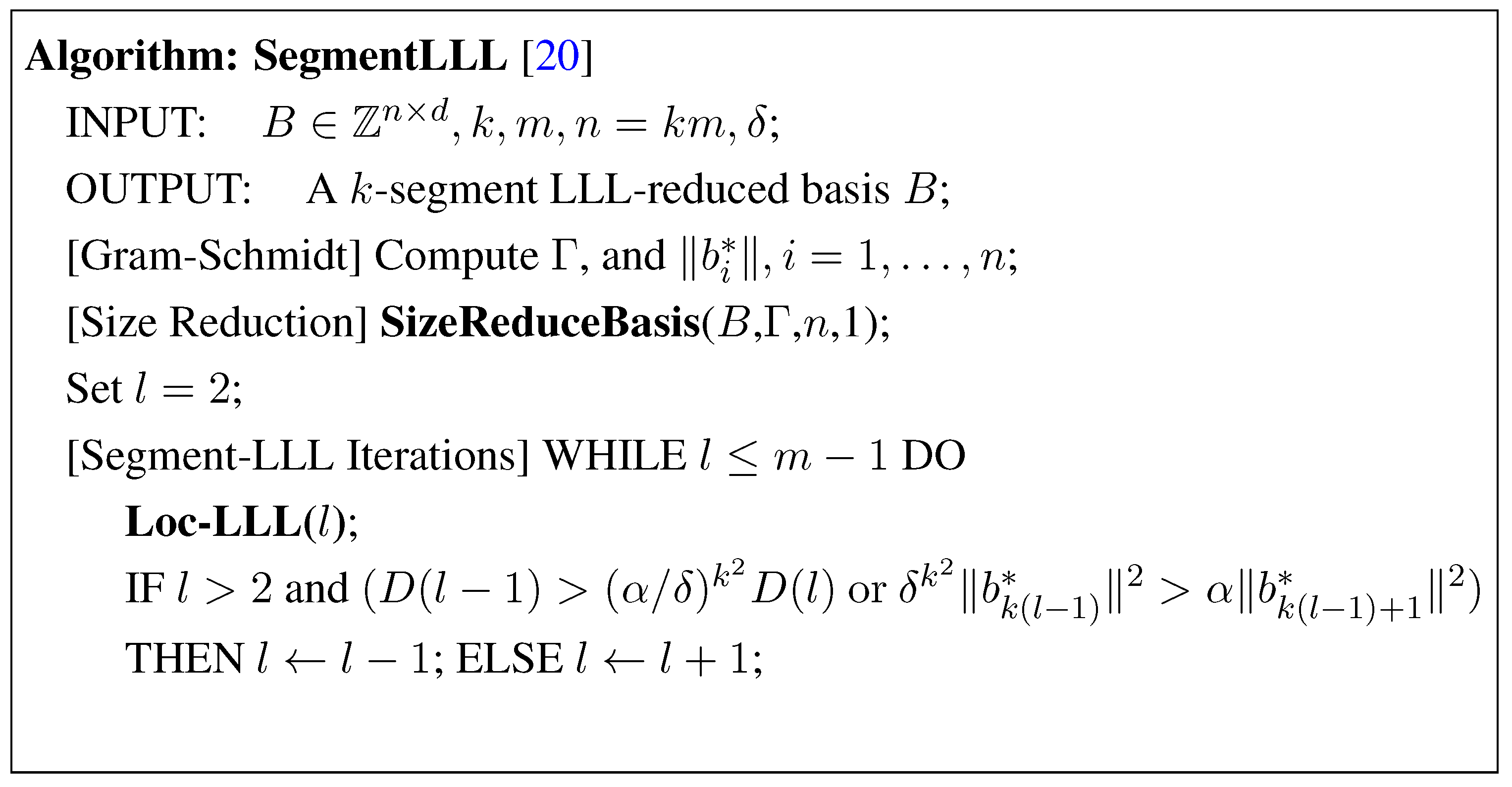
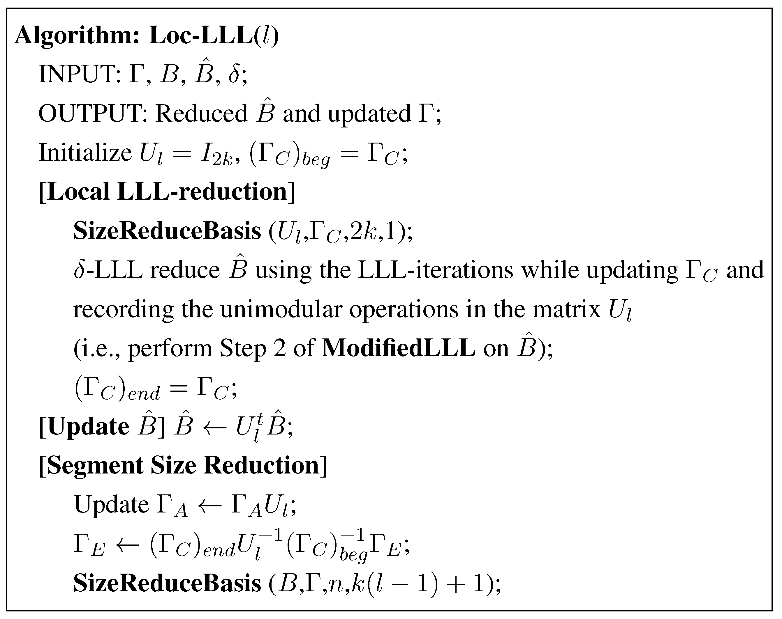
Recently Koy and Schnorr [20] introduced the concept of a segment LLL reduced basis (See Definition D7), and gave an algorithm for finding such a basis. The segment LLL reduced basis satisfies a slightly weaker condition, however, it is computed by Koy and Schnorr [20] in $O\left(n\right)$ fewer arithmetic operations. The algorithm of Koy and Schnorr works on two segments of B, i.e., $[B_{l-1},B_l]=[b_{k(l-1)+1},\dots ,b_{k(l+1)}]$ at a time. This algorithm is outlined in Figure 10. The work in the SegmentLLL algorithm comes from the calls to a subroutine Loc-LLL(l) given in Figure 11. Subroutine Loc-LLL(l) performs a local LLL basis reduction on the segment [$B_{l-1},B_l]$ and records the operations in a unimodular matrix $U_l\in {\mathbb{Z}}^{2k\times 2k}$, as explained below.

Figure 10. The Segment LLL Basis Reduction Algorithm.

Figure 10. The Segment LLL Basis Reduction Algorithm.

The Local-LLL reduction (Subroutine Loc-LLL(l)) works on $\widehat{B}:={[B_{l-1},B_l]}^t$ and Γ. The matrix Γ in (4.6) is partitioned into segments with each segment has $2k$ basis vectors.

$$\Gamma =\left[\begin{array}{ccc}\begin{array}{ccc}1\hfill & \dots \hfill & {\Gamma }_{1,k(l-1)}\hfill \\ & \ddots \hfill & ⋮\hfill \\ & & 1\hfill \end{array}\hfill & \begin{array}{ccc}{\Gamma }_{1,k(l-1)+1}\hfill & \dots \hfill & {\Gamma }_{1,k(l+1)}\hfill \\ ⋮\hfill & & ⋮\hfill \\ {\Gamma }_{k(l-1),k(l-1)+1}\hfill & \dots \hfill & {\Gamma }_{k(l-1),k(l+1)}\hfill \end{array}\hfill & \begin{array}{ccc}{\Gamma }_{1,k(l+1)+1}\hfill & \dots \hfill & {\Gamma }_{1,n}\hfill \\ ⋮\hfill & & ⋮\hfill \\ {\Gamma }_{k(l-1),k(l+1)+1}\hfill & \dots \hfill & {\Gamma }_{k(l-1),n}\hfill \end{array}\hfill \\ \begin{array}{ccc}& & \\ & & \\ & & \end{array}\hfill & \begin{array}{ccc}1\hfill & \dots \hfill & {\Gamma }_{k(l-1)+1,k(l+1)}\hfill \\ & \ddots \hfill & ⋮\hfill \\ & & 1\hfill \end{array}\hfill & \begin{array}{ccc}{\Gamma }_{k(l-1)+1,k(l+1)+1}\hfill & \dots \hfill & {\Gamma }_{k(l-1)+1,n}\hfill \\ ⋮\hfill & & ⋮\hfill \\ {\Gamma }_{k(l+1),k(l+1)+1}\hfill & \dots \hfill & {\Gamma }_{k(l+1),n}\hfill \end{array}\hfill \\ \begin{array}{ccc}& & \\ & & \\ & & \end{array}\hfill & \begin{array}{ccc}& & \\ & & \\ & & \end{array}\hfill & \begin{array}{ccc}1\hfill & \dots \hfill & {\Gamma }_{k(l+1)+1,n}\hfill \hfill \\ & \ddots \hfill & ⋮\hfill \\ & & 1\hfill \end{array}\hfill \end{array}\right]$$

$$\equiv \left[\begin{array}{ccc}& {\Gamma }_A& \\ & {\Gamma }_C& {\Gamma }_E\\ & & \end{array}\right]$$

(4.6)

Figure 11. The Local LLL Iterations.

Figure 11. The Local LLL Iterations.

When working in Loc-LLL(l) all LLL swaps and size reductions are restricted to the input $2k$ segment. Only the matrix ${\Gamma }_C$ is updated while performing the segment LLL swaps and size reductions. The unimodular operations updating ${\Gamma }_A$, and the operations required to update ${\Gamma }_E$ are stored in the matrix $U_l$. The updates for ${\Gamma }_A$ and ${\Gamma }_E$ are performed only after it is no longer possible to perform an LLL-swap based on the information in ${\Gamma }_C$. ${\Gamma }_A$ and ${\Gamma }_E$ are updated as follows:

$${\Gamma }_A={\Gamma }_A{U}_l,{\Gamma }_E={\left({\Gamma }_C\right)}_{end}{U}_l^{-1}{\left({\Gamma }_C\right)}_{beg}^{-1}{\Gamma }_E$$

Here ${\left({\Gamma }_C\right)}_{beg}$ and ${\left({\Gamma }_C\right)}_{end}$ are ${\Gamma }_C$ matrices recorded at the beginning and end of the Local LLL-reduction step in Loc-LLL(l). Since only matrix ${\Gamma }_C$ is updated during the LLL unimodular operations in this segment the corresponding updates of ${\Gamma }_C$ and $U_l$ are performed using $O\left(k^2\right)$ arithmetic operations. The total number of swaps in all calls to Loc-LLL(l) is bounded by $O\left(n{log}_{1/\delta }{M}_{sc}\right)$, hence the total work in the Local LLL-reduction step is bounded by $O\left(n{k}^2{log}_{1/\delta }{M}_{sc}\right)$ arithmetic operations. The cost of updating ${\Gamma }_A$ and ${\Gamma }_C$, and performing the Segment Size Reduction step in each execution of Loc-LLL(l) is $O\left(ndk\right)$ arithmetic operations.

Let $decr$ denote the number of times that the condition

$$(D(l-1)>{(\alpha /\delta )}^{k^2}D\left(l\right)\mathrm{or}{\delta }^{k^2}\parallel b_{k(l-1)}^{*}{\parallel }^2>\alpha \parallel b_{k(l-1)+1}^{*}{\parallel }^2)$$

holds and l is decreased. The number of times Loc-LLL(l) is called is $m-1+2·decr$. Koy and Schnorr [20] showed that $decr\le 2\frac{m-1}{k^2}{log}_{1/\delta }{M}_{sc}<2\frac{n}{k^3}{log}_{1/\delta }{M}_{sc}$. Hence the total work in the Segment Size Reduction step of Loc-LLL(l) is $O\left(\frac{n^3}{k^2}{log}_{1/\delta }{M}_{sc}\right)$ arithmetic operations when $d=O\left(n\right)$. This leads to the computational complexity result in Table 1 when $k=\sqrt{n}$ and $d=O\left(n\right)$. We have omitted details on the bounds on the length of the elements in $U_l$ and Γ (see Koy and Schnorr [20] for details).

5. The Modular Segment LLL Reduction with Modular Arithmetic

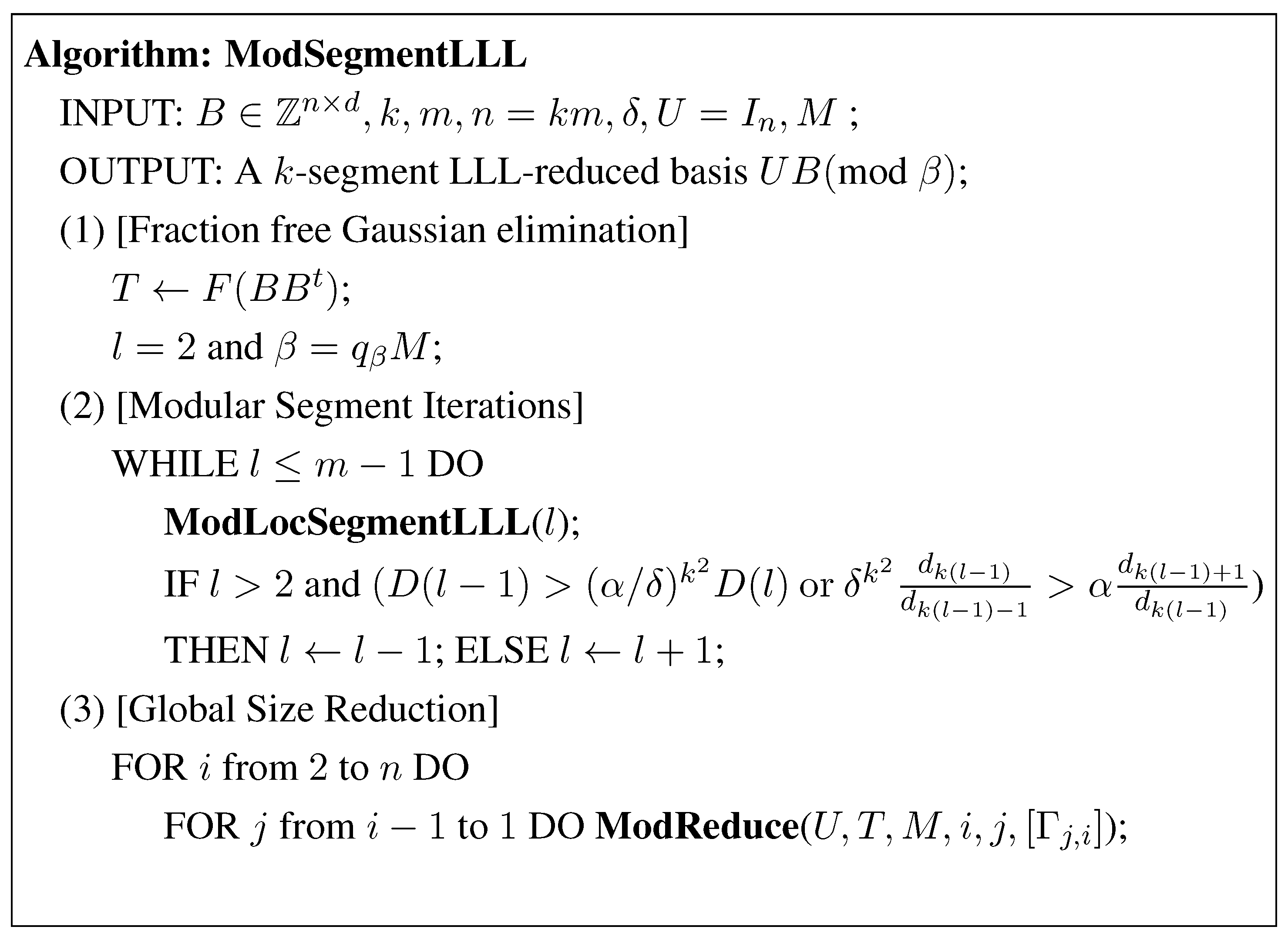
5.1. Algorithm and Its Complexity

We are now in a position to give our segment LLL reduction algorithm with modular arithmetic. It finds a segment LLL reduced basis with an $O\left(n^{0.5}\right)$ improvement in the computational complexity when $M_{sc}=2^{O\left(n^2\right)}$. This algorithm is given in Figure 12. The major difference in the ModSegmentLLL and SegmentLLL algorithms is in performing the ModLocSegmentLLL step presented in Figure 13. In this subroutine we perform updates using modular arithmetic while working with $\widehat{B}$. The subroutines ModReduce and ModSwap require $O\left(k\right)$ operations in comparison to the $O\left(k^2\right)$ worst case operations in the algorithm of Koy and Schnorr described in the previous section.

Figure 12. The Modular Segment LLL Basis Reduction.

Figure 12. The Modular Segment LLL Basis Reduction.

Figure 13. The Modular Local Segment LLL Basis Reduction.

Figure 13. The Modular Local Segment LLL Basis Reduction.

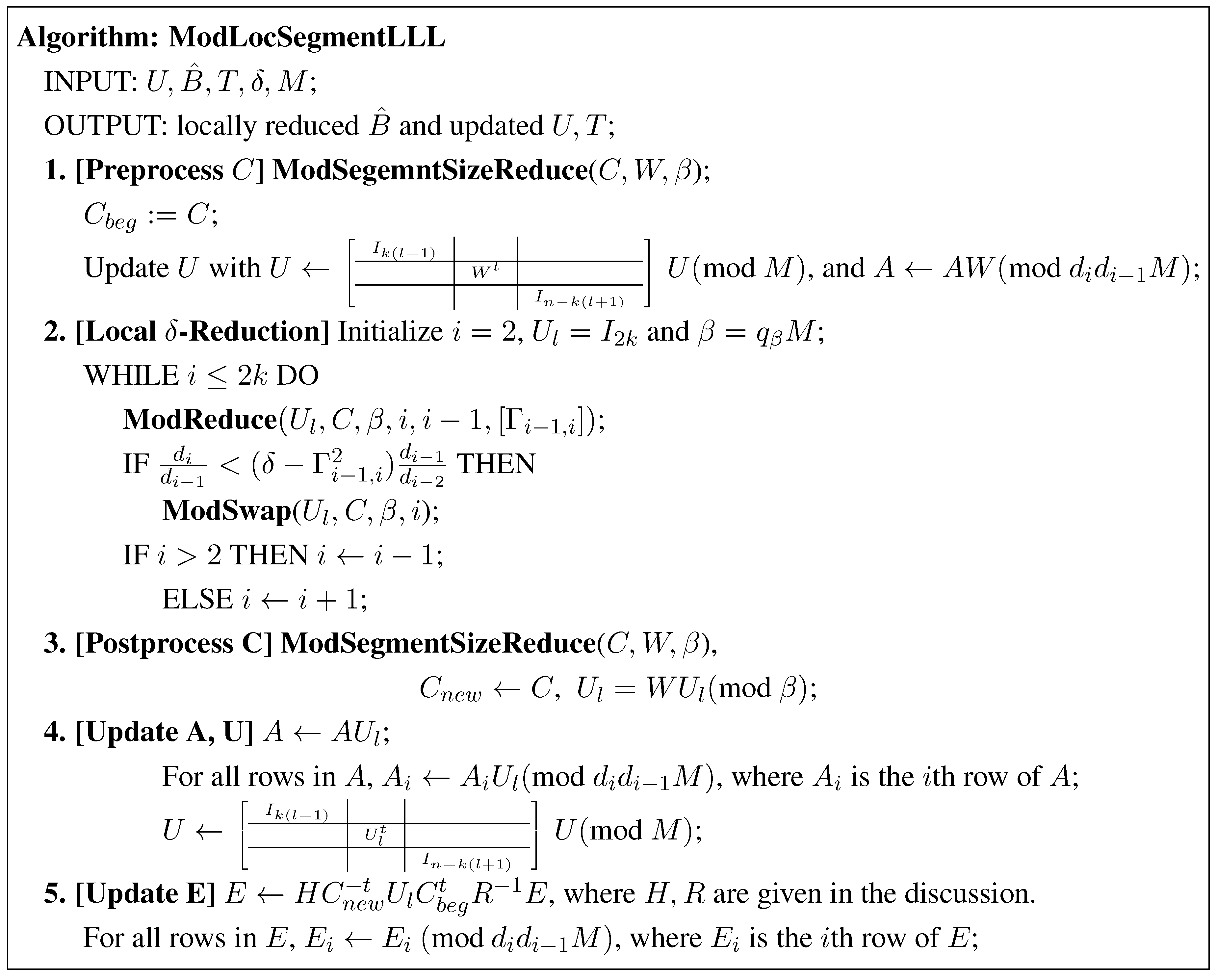
Figure 14. Size Reduction of a Segment Using Modular Arithmetic.

Figure 14. Size Reduction of a Segment Using Modular Arithmetic.

We now explain the steps in ModLocSegmentLLL. While working with the matrix $\widehat{B}$, let us partition

$$T=\left[\begin{array}{ccc}& A& \\ & C& E\\ & & \end{array}\right]$$

similar to the partitioning of Γ in (4.6). We perform two types of unimodular operations on $\widehat{B}$ in the ModLocSegmentLLL algorithm. The Preprocess C and Postprocess C steps are performed to ensure that the lattice basis vectors corresponding to C are size reduced before and after performing the Local δ-Reduction step. This allows us to bound the size of matrix Q needed to update E after completing the Local δ-Reduction step.

The calls to ModReduce and ModSwap are as in the case of the ModularLLL algorithm with the important difference that they are now performed on a segment. ModReduce subtracts a multiple of a row (column) from another row (column). This unimodular operation is recorded by updating $U_l$ modulo β. The constant β used in the ModSegmentLLL algorithm is taken to be a multiple of M. A choice of β is specified below in Lemma 4. This inferior value is used in the intermediate computations because during the algorithm we don’t have a bound on the elements of $\widehat{B}$. However, the fact that the initial and terminating $\widehat{B}$ are size reduced ensures that a proper bound on β is still possible. The subroutine ModSwap performs all necessary computations to update C and $U_l$ when two rows of $\widehat{B}$ are swapped. The elements of C are recorded modulo $d_i{d}_{i-1}\beta$. As in the case of Storjohann’s modification of the LLL algorithm, there is no need to record the modulo operations in $U_l$.

The matrix $U_l$ is further updated in the Postprocess C step by incorporating all the unimodular transformations recorded in W while working on the size reduction of the basis vectors corresponding to C. Here the elements of $U_l$ are recorded modulo β. Note that while $U_l$ is recorded modulo β, U is recorded modulo M. Updating A and U is straightforward. In Section 5.2 we show that the computations involving $U_l$ and A can be performed with integers of $O(ln{M}_{sc})$ bit length. To this end we use the results from Storjohann [14] for his analysis of the semi-reduction algorithm.

The total computational effort in Steps 1, 3, 4, and 5 of the ModLocSegmentLLL algorithm is $O\left(n{k}^2\right)$ arithmetic operations. Following [20] and [14, Theorem 18], there are at most $n\left({log}_{1/\delta }{M}_{sc}\right)$ swaps in all the executions of the ModLocSegmentLLL algorithm, each swap requiring $O\left(k\right)$ arithmetic operations. Hence, we improve the total computational efforts in Step 2 [Modular Segment Iterations] of the ModSegmentLLL algorithm to $O\left(nk{log}_{1/\delta }{M}_{sc}\right)$ arithmetic operations. Since there are a total of $O\left(\frac{n}{k^3}{log}_{1/\delta }{M}_{sc}\right)$ calls to the ModLocSegmentLLL algorithm we are led to the following theorem.

Theorem 1 

Using standard matrix multiplication, for $k=O\left(\sqrt{n}\right)$ and $d=O\left(n\right)$, Step 2 of Algorithm ModSegmentLLL performs $O\left(n^{1.5}{log}_{1/\delta }{M}_{sc}\right)$ arithmetic computations. We can perform these computations using integers of bit length $O(ln{M}_{sc})$.

The proof of the first statement in Theorem 1 is already complete. The second statement on the bit length needed for computations in proved in Section 5.2. We note that Step 1 of the ModSegmentLLL algorithm computes F and T, and Step 3 performs a global size reduction. Step 1 is performed in $O\left(n^3\right)$ arithmetic operations on integers of bit length $O(ln{M}_{sc})$ [14]. Step 3 is also performed in $O\left(n^3\right)$ arithmetic operations on integers of bit length $O(ln{M}_{sc})$. Therefore, we have the following corollary.

Corollary 1 

For a basis $b_1,\dots ,b_n\in {\mathbb{Z}}^d$ and $d=O\left(n\right)$, the running time of Algorithm ModSegmentLLL is bounded by $O\left(n^{1.5}{log}_{1/\delta }{M}_{sc}\right)$ arithmetic operations using integers of bit length $O(ln{M}_{sc})$.

The bound in Corollary 1 is $n^{0.5}$ better than the bound in Algorithm SegmentLLL when $M_{sc}=2^{O\left(n^2\right)}$, which is possible in the worst case. Section 5.2 is devoted to showing the correctness of Algorithm ModSegmentLLL and proving Theorem 1.

5.2. Correctness of the ModSegmentLLL Algorithm

The following lemma allows us to compute U modulo M, and T modulo $d_i{d}_{i-1}M$ during the ModSegmentLLL algorithm.

Lemma 3 

Upon termination, the reduced basis from the SegmentLLL and ModSegmentLLL algorithms has the following upper bound

$$\parallel b_i{\parallel }^2\le n{M}_0\text{for}1\le i\le n,\text{and}\parallel b_i^{*}\parallel \le M_0$$

throughout the algorithm.

Proof: 

Follow the proof of Lemma 2, while observing that size reduction or modular reduction of the elements in T leave $\parallel b_i^{*}\parallel$ unchanged. ☐

The following lemma of Schönhage allows to give a proper value of β, which is used to reduce the entries of $U_l$ and C modulo β. We now show that $U_l$, A, C, and E are correctly updated using integers of $O(ln{M}_{sc})$ bits.

Lemma 4 

[8] Let ${\widehat{B}}_{beg}$, ${\widehat{B}}_{end}\in {\mathbb{Z}}^{2k\times d}$ be size-reduced bases. The unimodular matrix $\widehat{U}$ that transforms ${\widehat{B}}_{beg}$ to ${\widehat{B}}_{end}$, satisfies

$$\parallel \widehat{U}{\parallel }_1\le {\left(2k\right)}^2{\left(\frac{3}{2}\right)}^{2k-1}{M}_{sc}\le M_{sc}^2$$

where $\parallel \widehat{U}{\parallel }_1={max}_j\{\parallel {\widehat{U}}_j^t{\parallel }_1\}$ and ${\widehat{U}}_j^t$ is the j-th column of $\widehat{U}$.

Lemma 4 allows to take $\beta =q_{\beta }M$, where $q_{\beta }=[(2\lceil M_{sc}^2\rceil +1)/M]+1$ while reducing the entries of $U_l$ modulo β. Note that taking β as a multiple of M is important because $U_l$ is used to update U whose elements are computed modulo M.

Updating E

Let R be the $2k\times 2k$ diagonal matrix with the i-th diagonal entry $d_{k(l-1)+i}{d}_{k(l-1)+i-1}$ for $1\le i\le 2k$, and H the $2k\times 2k$ diagonal matrix with $H_{1,1}={\left(C_{new}\right)}_{1,1}{d}_{k(l-1)}$ and $H_{i,i}={\left(C_{new}\right)}_{i,i}{\left(C_{new}\right)}_{i-1,i-1}$ for $2\le i\le 2k$, where $d_{k(l-1)+i},1\le i\le 2k$ are the diagonal entries of $C_{beg}$. Following Storjohann’s development of his algorithm for finding a semi-reduced basis in [14, Equation (29)], we can show that the matrix E is updated by

$$\tilde{E}=QE,\text{where}Q=\frac{1}{d_{k(l-1)}}H{\left(C_{new}^{-1}\right)}^t{U}_l{d}_{k(l-1)}{C}_{beg}^t{R}^{-1}$$

These computations are performed in a specific order to maintain integrality of operations: (i) backtrack fraction free Gaussian elimination by pre-multiplying E by $d_{k(l-1)}{C}_{beg}^t{R}^{-1}$; (ii) pre-multiply by the basis modular transformation matrix $U_l$; (iii) forwardtrack fraction free Gaussian elimination by pre-multiplying the result from (ii) by $(1/d_{k(l-1)})H{\left(C_{new}^{-1}\right)}^t$.

To establish a bound on the magnitudes of the integers in $\tilde{E}$, we need to bound $\parallel C_{new}^{-1}{\parallel }_{\infty }$. Let S be the $2k\times 2k$ diagonal matrix with the i-th diagonal entry ${\left(C_{new}\right)}_{i,i}$ for $1\le i\le 2k$ so that $S^{-1}{C}_{new}$ is unit upper triangular with all off diagonal entries $\le 1/2$, (Recall that the basis vectors corresponding to $C_{new}$ are size-reduced). In particular, the entries in ${\left(S^{-1}{C}_{new}\right)}^{-1}$ are $2k\times 2k$ minors of $\left(S^{-1}{C}_{new}\right)$ which is bounded by ${\left(2k\right)}^k$ using Hadamard’s inequality. It follows that the entries in $C_{new}^{-1}={\left(S^{-1}{C}_{new}\right)}^{-1}{S}^{-1}$ are bounded by ${\left(2k\right)}^k$ because $d_i\ge 1,1\le i\le n$. We get

$$\begin{array}{cc}\hfill \parallel \tilde{E}{\parallel }_{\infty }={\parallel QE\parallel }_{\infty }& \le {\left(2k\right)}^3{\parallel H\parallel }_{\infty }\parallel C_{new}^{-1}{\parallel }_{\infty }\parallel U_l{\parallel }_{\infty }{\parallel C_{beg}^t\parallel }_{\infty }\beta \hfill \end{array}$$

$$\begin{array}{cc}& \le {\left(2k\right)}^3{M}_{sc}^2{\left(2k\right)}^k{\left(2k\right)}^2{(3/2)}^{2k-1}{M}_{sc}{M}_{sc}\beta \hfill \end{array}$$

$$\begin{array}{cc}& \le 2{\left(2k\right)}^{k+5}{(3/2)}^{2k-1}{M}_{sc}^6\hfill \end{array}$$

(5.7)

The above inequality shows that the entries of $\tilde{E}$ are bounded by $O(ln{M}_{sc}+klnk)$ bit length. Furthermore, if $\tilde{E}$ is computed by multiplying E with matrices in Q from right to left, then all intermediate matrices are fraction free, and the computations are performed on integers of size $O(ln{M}_{sc})$. This completes the proof for the correctness of the algorithm.

5.3. The Modular Segment LLL using Fast Matrix Multiplication

The complexity of Step 2 of the ModSegmentLLL algorithm is bounded by the following theorem when using fast matrix multiplication.

Theorem 2 

If $d=O\left(n\right)$, $k=\lceil n^{\frac{1}{5-\theta }}\rceil$, then using fast matrix multiplications Step 2 of the ModSegmentLLL algorithm can be performed in $O\left(n^{1+\frac{1}{5-\theta }}\left({log}_{1/\delta }{M}_{sc}\right)\right)$ operations using integers of bit length $O\left({log}_2{M}_{sc}\right)$.

Proof: 

As discussed above, there are at most $n\left({log}_{1/\delta }{M}_{sc}\right)$ LLL-exchanges, each requiring $O\left(k\right)$ arithmetic operations for a local δ-reduction. According to [20, Theorem 3], there are $decr\le 2\frac{n}{k^3}{log}_{1/\delta }{M}_{sc}$ calls of the ModLocSegmentLLL algorithm. Each call requires $O(n{k}^{\theta -1}+nk+k^2(lnk))$ arithmetic operations for updating matrices A and T. The complexity of Step 2 of the ModSegmentLLL algorithm is bounded by

$$\begin{array}{cc}& O\left(nk\left({log}_{1/\delta }{M}_{sc}\right)\right)+O\left(2\frac{n}{k^3}\left({log}_{1/\delta }{M}_{sc}\right)(n{k}^{\theta -1}+nk+k^2\left({log}_{2}k\right))\right)\hfill \\ \hfill \le & O\left(nk\left({log}_{1/\delta }{M}_{sc}\right)\right)+O\left(\frac{n^2}{k^{4-\theta }}\left({log}_{1/\delta }{M}_{sc}\right)\right)\hfill \\ \hfill =& O\left(n^{1+\frac{1}{5-\theta }}\left({log}_{1/\delta }{M}_{sc}\right)\right)\hfill \end{array}$$

when $k=\lceil n^{\frac{1}{(5-\theta )}}\rceil$. ☐

Storjohann [14] showed that the fraction free Gaussian elimination and Step 3 of the algorithm can be performed in $O(n^{\theta }logn)$ arithmetic operations for $\theta =2.376$ with integers of bit length $O(ln{M}_{sc})$. The bound in Theorem 2 is $O\left(n^{1.382}\left({log}_{1/\delta }{M}_{sc}\right)\right)$ where $M_{sc}>2^n$. Hence Step 2 of Algorithm ModSegmentLLL dominates the overall effort giving the following corollary.

Corollary 2 

For $d=O\left(n\right)$, and $k=\lceil n^{\frac{1}{(5-\theta )}}\rceil$ the running time of Algorithm ModSegmentLLL is bounded by $O\left(n^{1.382}{log}_{1/\delta }{M}_{sc}\right)$ operations using integers of bit length $O(ln{M}_{sc})$ when using fast matrix multiplication.

6. Concluding Remarks

Schnorr [17, Section 6] remarked that it is possible to further improve the running time of the iterated subsegment algorithm in [17] using modular arithmetic. This is possible since the iterated subsegment algorithm runs in $O(n^{3}lnn)$ operations by recursively transporting local transforms from a segment-level to the next higher segment. Note that by comparison the basic segment-LLL algorithm analyzed in this paper requires $O\left(n^{3.5}\right)$ operations while using standard arithmetic, and $O(n^{3+\frac{1}{5-\theta }})$ operations while using fast matrix multiplications. In all cases the modular arithmetic computations are performed on numbers of length $O\left(n^2\right)$. Unfortunately the worst-case $O\left(n^2\right)$ bit-length required for the modular arithmetic is large, and floating point arithmetic is more practical. Numerical experience using implementations based on floating point arithmetic were reported in [23] for the LLL algorithm and in [11] for the segment-LLL reduction algorithm. The possibility of combining modular arithmetic with floating point computations remains a topic of future research.

References

- Cassels, J.W.S. An Introduction to the Geometry of Numbers; Springer-Verlag: Berlin, Germany, 1971. [Google Scholar]
- Dwork, C. Lattices and their application to cryptography. Availible online: http://www.dim.uchile.cl/m̃kiwi/topicos/00/dwork-lattice-lectures.ps (accessed on 15 June 2010).
- Lenstra, H.W. Integer programming with a fixed number of variables. Math. Operat. Res. 1983, 8, 538–548. [Google Scholar] [CrossRef]
- Ajtai, M. The shortest vector problem in L2 is NP-hard for randomized reductions. In Proceedings of the 30th ACM Symposium on Theory of Computing, Dallas, TX, USA, May 1998; pp. 10–19.
- Micciancio, D. The shortest vector in a lattice is hard to approximate to within some constant. SIAM J. Comput. 2001, 30, 2008–2035. [Google Scholar] [CrossRef]
- van Emde Boas, P. Another NP-complete partition problem and the complexity of computing short vectors in lattices; Technical report MI-UvA-81-04; University of Amsterdam: Amsterdam, The Netherlands, 1981. [Google Scholar]
- Lenstra, A.K.; Lenstra, H.W.; Lovász, L. Factoring polynomials with rational coefficients. Math. Ann. 1982, 261, 515–534. [Google Scholar] [CrossRef]
- Schönhage, A. Factorization of univariate integer polynomials by diophantine approximation and improved lattice basis reduction algorithm. In Proceedings of 11th Colloquium Automata, Languages and Programming; Springer-Verlag: Antwerpen, Belgium, 1984; LNCS 172, pp. 436–447. [Google Scholar]
- Kannan, R. Improved algorithms for integer programming and related lattice problems. In Proceedings of the 15th Annual ACM Symposium On Theory of Computing, Boston, MA, USA, May 1983; pp. 193–206.
- Schnorr, C.P. A hierarchy of polynomial time lattice basis reduction algorithms. Theor. Comput. Sci. 1987, 53, 201–224. [Google Scholar] [CrossRef]
- Koy, H.; Schnorr, C.P. Segment LLL-reduction with floating point orthogonalization. LNCS 2001, 2146, 81–96. [Google Scholar]
- Hermite, C. Second letter to Jacobi. Crelle J. 1850, 40, 279–290. [Google Scholar] [CrossRef]
- Schnorr, C.P. A more efficient algorithm for lattice basis reduction. J. Algorithms 1988, 9, 47–62. [Google Scholar] [CrossRef]
- Storjohann, A. Faster Algorithms for Integer Lattice Basis Reduction; Technical Report 249; Swiss Federal Institute of Technology: Zurich, Switzerland, 1996. [Google Scholar]
- Schnorr, C.P. Block Korkin-Zolotarev Bases and Suceessive Minima; Technical Report 92-063; University of California at Berkley: Berkley, CA, USA, 1992. [Google Scholar]
- Nguyen, P.Q.; Stehlé, D. Floating-point LLL revisited. LCNS 2005, 3494, 215–233. [Google Scholar]
- Schnorr, C.P. Fast LLL-type lattice reduction. Inf. Comput. 2006, 204, 1–25. [Google Scholar] [CrossRef]
- Kaib, M.; Ritter, H. Block Reduction for Arbitrary Norms. Availible online: http://www.mi.informatik.uni-frankfurt.de/research/papers.html (accessed on 15 June 2010).
- Lovász, L.; Scarf, H. The generalized basis reduction algorithm. Math. Operat. Res. 1992, 17, 754–764. [Google Scholar] [CrossRef]
- Koy, H.; Schnorr, C.P. Segment LLL-reduction of lattice bases. LNCS 2001, 2146, 67–80. [Google Scholar]
- Geddes, K.O.; Czapor, S.R.; Labahn, G. Algorithms for Computer Algebra; Kluwer: Boston, MA, USA, 1992. [Google Scholar]
- Coppersmith, D.; Winograd, S. Matrix multiplication via arithmetic progressions. J. Symbol. Comput. 1990, 9, 251–280. [Google Scholar] [CrossRef]
- Stehlé, D. Floating-point LLL: Theoretical and practical aspects. In The LLL Algorithm; Springer-verlag: New York, NY, USA, 2009; Chapter 5. [Google Scholar]
- Schönhage, A.; Strassen, V. Schnelle Multiplikation grosser Zahlen. Computing 1971, 7, 281–292. [Google Scholar] [CrossRef]
© 2010 by the authors; licensee MDPI, Basel, Switzerland. This article is an Open Access article distributed under the terms and conditions of the Creative Commons Attribution license http://creativecommons.org/licenses/by/3.0/.
Share and Cite
MDPI and ACS Style
Mehrotra, S.; Li, Z. Segment LLL Reduction of Lattice Bases Using Modular Arithmetic. Algorithms 2010, 3, 224-243. https://doi.org/10.3390/a3030224
AMA Style
Mehrotra S, Li Z. Segment LLL Reduction of Lattice Bases Using Modular Arithmetic. Algorithms. 2010; 3(3):224-243. https://doi.org/10.3390/a3030224
Chicago/Turabian StyleMehrotra, Sanjay, and Zhifeng Li. 2010. "Segment LLL Reduction of Lattice Bases Using Modular Arithmetic" Algorithms 3, no. 3: 224-243. https://doi.org/10.3390/a3030224