Fluidsim: A Car Traffic Simulation Prototype Based on FluidDynamic

Abstract

We present a car traffic simulation prototype for complex networks, that is formed by a collection of roads and junctions. Traffic load evolution is described by a model based on fluid dynamic conservation laws, deduced from conservation of the number of cars. The model contains some additional hypothesis in order to reproduce specific car traffic features such as route based car distribution at nodes and the presence of right-of-way at the crossroads. A complete implementation of this model is then presented, together with computational results on case studies.

1. Introduction

Modeling and simulation methods are essential elements in the design and operation of transportation systems. Congestion problems in cities worldwide have prompted at all levels of government and industry a proliferation of interest in Intelligent Transportation Systems (ITS) that include advanced supply and demand management techniques. Such techniques include real-time traffic control measures and real-time traveler information and guidance systems whose purpose is to assist travelers in making departure time, mode and route choice decisions. Transportation researchers have developed models and simulators for use in the planning, design and operations of such systems (see, e.g., [1,2,3,4,5,6,7,8,9,10]).

There is great potential for useful application of microsimulation models to the analysis of complex traffic problems in urban areas, alongside the analytical techniques that are in use. Microsimulation is useful due to increasing levels of system complexity and uncertainty involved in the operation of urban traffic networks. However, concerns are often expressed regarding misuse of microsimulation. Response to a survey of microsimulation model users was summarised as “microsimulation is useful but dangerous” [1].

Several key components of traffic models are discussed in the literature, and various recommendations are made, with a view to improving the practical usefulness of microsimulation models. These include:

• the use of simulation for capacity analysis, including the dependence of capacity on demand flow rates;
• modelling of queue discharge (saturation) flow rate, queue discharge speed and other queue discharge parameters at signalised intersections, and relating them to the general queuing, acceleration and car-following models used in microsimulation;
• modelling of gap-acceptance situations at all types of traffic facilities, and
• estimation of lane flows at intersection approaches, and relating this to lane changing models used in microsimulation.

We start from these considerations and in this paper we propose a prototype of a traffic simulation model, based on fluid dynamics models in order to reproduce the macroscopic within-day evolution of heavy traffic flows across a urban network. The software prototype is based on a complete model developed starting from some basic results on the application of scalar hyperbolic conservation laws in order to describe the conservation of car flows on a single road. Such results, known since the 1950s thanks to Lighthill-Whitham [11] and Richards [12] contributions, were extended with a complete theory in [13,14] to the case of traffic networks with a finite number of roads meeting at junctions. Similar approaches were developed independently and related results and extensions can be found in [15,16,17,18,19,20]. The model assumes that distribution of traffic flows at nodes (junctions) is known in advance, and that cars behaviour is such that the throughput at nodes is maximized, subject to the constraints imposed by conservation laws at nodes. Right-of-way coefficients are used in this context to break ties among different roads incoming in a junction.

Such model is particularly effective to deal with different type of data sources, such as coils [21], mobile GPS phones [22] and clear boxes [23].

The paper is organized as follows. In Section 2, the model is described in more detail, together with some sketches on the numerical methods considered in the simulation prototype. In Section 3, the scheme of the simulation prototype and implementation details are presented. Finally, in Section 4, we provide computational results on networks of different sizes in order to evaluate computational effort needed by the software when some basic parameters are varied.

2. A Fluid Dynamics Model for Traffic Simulation

In order to introduce the way traffic evolution is treated in the application of fluid dynamics models, let us introduce some basic concepts that will be used in the following. A road network can be considered as a finite number of roads whose intersections are the junctions, or crossroads. A graph $G=(N,E)$, is used to represent such elements, N being the set of nodes related to the road junctions, while E is a set of arcs, or links, associated with the roads. The relationship between each element in N and E and their corresponding objects in the network is biunivocal, hence in this work we will use interchangeably nodes, junctions or crossroads, and roads, links or arcs.

In this particular case of link-and-node traffic network model, we deal with a continuous in space and time representation of the network, hence each arc $e_i$ is associated with a finite linear interval $[a_i,b_i]$, and the extreme points of this interval correspond to the head and tail nodes of the arc. This will turn out to be useful when dealing with the visual representation of the output. Indeed notice that each extreme point corresponds to a node in N. Then, given a geo-referencing for the entire set of nodes N, any point $p_i$ belonging to the interval $[a_i,b_i]$, associated with link $i\in E$, can be expressed by means of the coordinates of the first extreme point of the link, namely $a_i$, and the width of the interval $[a_i,p_i]$. We will implicitly use this concept in the output visualization on a GIS (Geographic Information System, see, e.g., [24]), when using the dynamic segmentation of arcs as described in Section 3.2.

For each node $v\in N$, we define the forward star $FS\left(v\right)\subset E$ as the set of arcs whose tail is node v, and the backward star $BS\left(v\right)\subset E$ as the set of arcs whose head is node v. The number of ingoing arcs is given by $\left|BS\left(v\right)\right|=b{s}_v$, and, similarly, the number of outgoing arcs $\left|FS\left(V\right)\right|=f{s}_v$. A node $n\in N$ is a source if $b{s}_n=0$, while is a sink node if $f{s}_n=0$. The macroscopic traffic variables considered in the model are the density of vehicles, the average speed of cars and the flow. Define $\rho =\rho (t,x)\in [0,{\rho }_{max}]$ as the density of cars, being $(t,x)\in {\mathbb{R}}^2$ and ${\rho }_{max}>0$ the maximum density of cars on the road. Define $f\left(\rho \right)=\rho ·v$ as the function representing the flow of cars, given by the density times the local average speed of cars $v=v(t,x)$. We assume, as done in most cases, that v is a decreasing function depending on the density only, and that the corresponding flow is a concave function. Moreover, we assume that f have a unique maximum and, for ease of notation, that ${\rho }_{max}=1$.

2.1. Traffic flows conservation on links

Here we recall the fluid dynamics model proposed in [11,12], which can be seen as a macroscopic within-day model allowing the observation of the time evolution of the traffic by means of the wave formation. On a single road, this nonlinear model is based on the conservation of car flows described by the following scalar hyperbolic conservation law:

$${\partial }_t\rho +{\partial }_{x}f\left(\rho \right)=0$$

(1)

Such a fluid dynamic model is widely considered as the most appropriate in order to detect macroscopic traffic flows phenomena such as shock formation and backward propagation of waves along roads. Some limits are known for these classic models concerning the spillback of traffic jams at nodes and the presence of discontinuities in a finite time, even starting from smooth initial data. Such drawbacks yield to the need for a careful definition of the analytical framework, taking into account the use of appropriate numerical schemes.

2.2. The model at junctions

The conservation of car flows at a junction can be written as the Rankine-Hugoniot relation, imposing an equal value for the sum of flows entering in and leaving from each node $n\in N$:

$$\sum _{i\in BS\left(n\right)}f\left({\rho }_i(t,b_i)\right)=\sum _{j\in FS\left(n\right)}f\left({\rho }_j(t,a_j)\right)\forall n\in N$$

(2)

where ${\rho }_i$, with $i\in BS\left(n\right)$, are the car densities on incoming roads while ${\rho }_j$, with $j\in FS\left(n\right)$, are the car densities on outgoing arcs.

Such a relationship cannot be directly applied on source nodes and sink nodes, and a set of boundary data have to be defined for each one of them, so that the corresponding boundary problem can be solved in order to reproduce car flows entering and leaving the whole traffic network.

The key problem is that conservation laws at a junction give rise to an underdetermined system, and some additional hypothesis must be introduced in order to determine a unique solution to the corresponding Riemann problem. Following [13], two main assumptions can be made in this sense:

(A)

Let us introduce a set of distribution coefficient, say α_ji, reproducing the behaviour of drivers at junctions n when choosing an outgoing road j ∈ FS(n) while coming from an ingoing road i ∈ BS(n). Such a set of coefficients give rise, for each node n different from a source and a sink, to the traffic distribution matrix:

$$A={\left\{a_{ji}\right\}}_{j\in FS\left(n\right),i\in BS\left(n\right)}.$$

In order to be feasible, at each junction n, distribution coefficients have to satisfy the following conditions:

$$\begin{array}{}\mathrm{(3)}& 0\le {\alpha }_{ji}\le 1,\forall i\in BS\left(n\right),\forall j\in FS\left(n\right)\hfill \mathrm{(4)}& \sum _{j\in FS\left(n\right)}{\alpha }_{ji}=1,\forall i\in BS\left(n\right)\hfill \end{array}$$

The distribution matrix elements can be considered as the turning ratios typically used in simulation environments to reproduce the choices of drivers at junctions. Such values can be obtained for instance by means of traffic detectors. On the other hand, it is always possible to compute turning ratios whenever an origin-destination (OD) matrix is available for the private car transportation demand, and a proper traffic assignment model can be applied on the considered network.

(B)

Subject to the conservation law in (2) and to condition (A), drivers behave in such a way to maximize the throughput at each node.

Let us now formulate a complete mathematical model for the solution of the Riemann problem at junctions. At each node n, given a certain density distribution over the incident arcs, we have to find a new feasible flow assignment for the extreme points of such arcs. We indicate with ${\gamma }_i,\forall i\in BS\left(n\right)$, and with ${\gamma }_j,\forall j\in FS\left(n\right)$, the new assignment of flows on the extreme points on the arcs incident to node n. Our aim is the maximization of the throughput at node n, that can be expressed interchangeably by either

$$max\sum _{i\in BS\left(n\right)}{\gamma }_i$$

or

$$max\sum _{j\in FS\left(n\right)}{\gamma }_j,$$

if one considers that the conservation relationships must hold. The set of constraints should take into account that the flow of cars crossing the junction and coming from each road must be less than or equal to the maximum flow assignment on the extreme point of the road itself, say ${\gamma }_i^{max},\forall i\in BS\left(n\right)$. Similar bounds can be expressed on the maximum flow that can be assigned on the extreme points of the outgoing arcs of the junctions, say ${\gamma }_j^{max},\forall j\in FS\left(n\right)$, if one considers the capacity of the arc.

Recalling all the conditions assumed until now, the problem can be formulated as a linear programming problem to be solved at each node n:

$$\begin{array}{ccc}& & maxz=\sum _{i\in BS\left(n\right)}{\gamma }_i\hfill \end{array}$$

(5)

$$\begin{array}{c}\hfill s.t.\end{array}$$

$$\begin{array}{}\mathrm{(6)}& 0\le {\gamma }_i\le {\gamma }_i^{max},\forall i\in BS\left(n\right)\hfill \mathrm{(7)}& 0\le \sum _{i\in BS\left(n\right)}{\alpha }_{ji}·{\gamma }_i\le {\gamma }_j^{max},\forall j\in FS\left(n\right)\hfill \end{array}$$

Notice that the left inequality in (7) is automatically satisfied using the first inequality in (6).

If some technical conditions on A hold true, then there exists a unique solution to such Linear Programming (briefly LP) problem. We refer the reader to the Appendix for details.

Right-of-way coefficient $q_i,\forall i\in BS\left(n\right)$, can now be introduced for each incoming road in such a way that $q_i>q_j$ if road $i\in BS\left(n\right)$ has right-of-way over road $j\in BS\left(n\right)$. (This represents also a way of selecting a unique solution if the technical conditions on A are not satisfied, cfr. the Appendix.) The model can be modified in order to accomplish with this new traffic feature:

$$\begin{array}{ccc}& & maxz=\sum _{i\in BS\left(n\right)}{q}_i·{\gamma }_i\hfill \end{array}$$

(8)

$$\begin{array}{c}\hfill s.t.\end{array}$$

$$\begin{array}{c}{\gamma }_i\le {\gamma }_i^{max},\forall i\in BS\left(n\right)\hfill \\ \sum _{i\in BS\left(n\right)}{\alpha }_{ji}·{\gamma }_i\le {\gamma }_j^{max},\forall j\in FS\left(n\right)\hfill \end{array}$$

The application of the right-of-way function in (8) when solving the Riemann problem at junctions could lead to a paradox in which the flow coming from a low priority road is completely blocked. In order to avoid this drawback, a driving aggressiveness coefficient can be introduced, say θ ∈ [0, 1], such that for a fraction θ of iterations the objective function (8) will be used, and the remaining iterations will use the objective function in (5). With respect to the model at junctions in [13], this new way of treating the right-of-way coefficients was introduced in order to develop a simulation prototype capable of tackling any kind of network, independently on the number of roads incident in a junction.

Existence and uniqueness conditions are discussed in the Appendix.

2.3. Numerical schemes

The solution of the Riemann problem on arcs is performed using numerical approximation schemes. In particular, in the first implementation of the software, three different numerical schemes were taken into account, the Godunov scheme, the 1-order Kinetic scheme, and the 2-order Kinetic scheme. The introduction of numerical approximation schemes requires the definition of a space step, say $\Delta s$, in such a way that the linear interval $[a_i,b_i]$ of length $l_i$, associated with an arc $i\in E$, is divided into a finite number of segments given by $\lfloor \frac{l_i}{\Delta s}\rfloor$. In Section 4, we present some tests concerning the computational time required by the use of these three different schemes, in order to find the appropriate trade-off between numerical accuracy and computational effort. The choice of Δs turns out to be a fundamental parameter in this sense. Let us now describe in more details the Godunov scheme, while we refer the reader to [25] for the other schemes.

Godunov scheme on a road network.

Now, in order to describe Godunov scheme we need to introduce a numerical grid with the following notation:

• Δs is the space grid size on each road I_i = [a_i, b_i];
• Δt is the time grid size on the time interval [0, T];
• (t_l, x_m) = (lΔt, mΔs), for l = 0, 1, ⋯, L and m = 0, 1, ⋯, M, are the grid points, with L and M, respectively, the number of time and space nodes of the grid.

For a function v defined on the grid we write $v_m^l=v(t_l,x_m)$. Notice that, in general, Δs may vary depending on the length of each road.

Godunov scheme is based on the local resolution to Riemann problems and it proceeds as follows. Piecewise constant approximations of the initial data are used as the initial data of Riemann problems. Waves in two neighbour cells do not interact before time Δt under the CFL condition $\Delta t\le \frac{1}{2{\lambda }_{max}}\Delta s$, where λ_max is the maximal speed of a wave, i.e. $max|f^{\prime }\left(\rho \right)|$. It is then possible to define a unique solution in the strip $(t_l,t_{l+1})\times \mathbb{R}$ by piecing the solutions obtained in each cell together. The exact solution is projected on a piecewise constant function $v_m^{l+1}=\frac{1}{\Delta s}{\int }_{x_m}^{x_{m+1}}{v}^{\Delta }(x,t_{l+1})dx,$ then the mean is obtained by the Gauss-Green formula, and this procedure is repeated recursively. Godunov scheme can be expressed in the conservative form as:

$$v_m^{l+1}=v_m^l-\frac{\Delta t}{\Delta s}\left(g^G(v_m^l,v_{m+1}^l)-g^G(v_{m-1}^l,v_m^l)\right),l=0,1,\cdots ,L-1,m=0,1,\cdots ,M,$$

(9)

with $g^G(u,v)$ the numerical flux. We assume that the flux function f is concave and has a unique maximum point σ, so that $f\left(\sigma \right)=f^{max}$. Then $g^G(u,v)$ is given by:

$$g^G(u,v)=\left\{\begin{array}{cc}min\left(f\right(u),f(v\left)\right)\hfill & \mathrm{if} u\le v,\hfill \\ \\ f\left(u\right)\hfill & \mathrm{if} v<u<\sigma ,\hfill \\ \\ f^{max}\hfill & \mathrm{if} v<\sigma <u,\hfill \\ \\ f\left(v\right)\hfill & \mathrm{if} \sigma <v<u.\hfill \end{array}\right.$$

Boundary conditions of the scheme are imposed for incoming road not linked on the left and for outgoing road not linked on the right.

Conditions at a junction.

For roads connected at the right endpoint, the interaction at a junction is taken into account as follows:

$$v_M^{l+1}=v_M^l-\frac{\Delta t}{\Delta s}\left({\widehat{\gamma }}_i-g^G(v_{M-1}^l,v_M^l)\right),$$

while for roads connected at the left endpoint we have:

$$v_0^{l+1}=v_0^l-\frac{\Delta t}{\Delta s}\left(g^G(v_0^l,v_1^l)-{\widehat{\gamma }}_j\right),$$

where ${\widehat{\gamma }}_i,{\widehat{\gamma }}_j$ are the maximized fluxes, respectively on incoming and outgoing roads, computed solving the linear programming problem of Section 2.2.

Other numerical schemes.

A particularly fast scheme was presented in [26]. This scheme is valid only when the flux is piecewise linear and the road network starts from an empty condition, and is based on strong properties of solutions. More precisely, one proves that there exists a unique regime change (from free flow to congested one) for every link of the network at any time. Then the scheme first traces the regime change and then solves linear problems in the rest of the link.

Such approach is very interesting for the highly reduced computational time. However, restrictions are non trivial. Beside the assumption on the special form of the flux function, the used strong properties of solutions represent a limit for the capability of describing real traffic and may fail to be satisfied by real data. We thus decided to use the more general approach based on the Godunov scheme in the present paper.

2.4. Computational complexity of the algorithm

The worst case analysis for the overall simulation algorithm can be provided as follows. The number of iterations directly depends on the ratio between the time interval and the size of the time-grid step, say T/Δt. Each iteration requires the solution of exactly |N| (the cardinality of N) linear programs at junctions. Even if the number of variables and constraints are bounded by O(|E|) in the theoretical worst case analysis, the algorithm is designed and developed to allow the simulation of the traffic evolution on road network, that presents a number of roads interesting each section that can be bounded by a very small constant, independently on the other characteristics of the specific road network (grid-like network). Therefore, it can be assumed that the computational effort required to solve each linear program at a junction is bounded by a constant K, independent on the size and the geometry of the considered road network. The complexity of solving the Riemann problem on the arcs can be indicated in turn by g(L/Δs), and, depending on the adopted scheme, grows polynomially (in general) with the density of the space-grid L/Δs. Hence, the algorithmic complexity of the simulation is bounded from above by the expression O((T/Δt)(|N|K + |E|g(L/Δs)). The computational effort will therefore increase linearly with the length of the considered time interval, and will be linearly influenced by the number |N| of roads and the number |E| of the junctions. It follows that, given the purposes of this work, concerning car traffic simulation on road (grid-like) networks, the specific geometries and topologies of the considered instances do not influence the computational time.

3. Implementing the FLUIDSIM Prototype

The simulation prototype, based on the model described in the previous section, is based on a main loop whose scheme is presented below.

1.	import network
2.	congestion reduction
	MAIN LOOP
3.	FOR t = 1 to iterations DO
4.	FOR each n ∈ N DO
5.	process node(n)
6.	ENDFOR
7.	FOR each e ∈ E DO
8.	process arc(n)
9.	ENDFOR
10.	export output(t)
11.	ENDFOR

At each iteration, two main routines are invoked, one providing the elaboration of each node and the other the processing of each arc. Since wave propagation speed is assumed to be finite, it is possible to compute the traffic evolution by processing elements separately. FLUIDSIM can be used as a macrosimulation tool in order to evaluate the general impact of some traffic regulation rules on the whole network. Therefore, data structures and other implementation details were chosen to guarantee the chance to consider a traffic network in its full generality, with a focus on the efficiency of processing large size instances, like those arising from real urban networks.

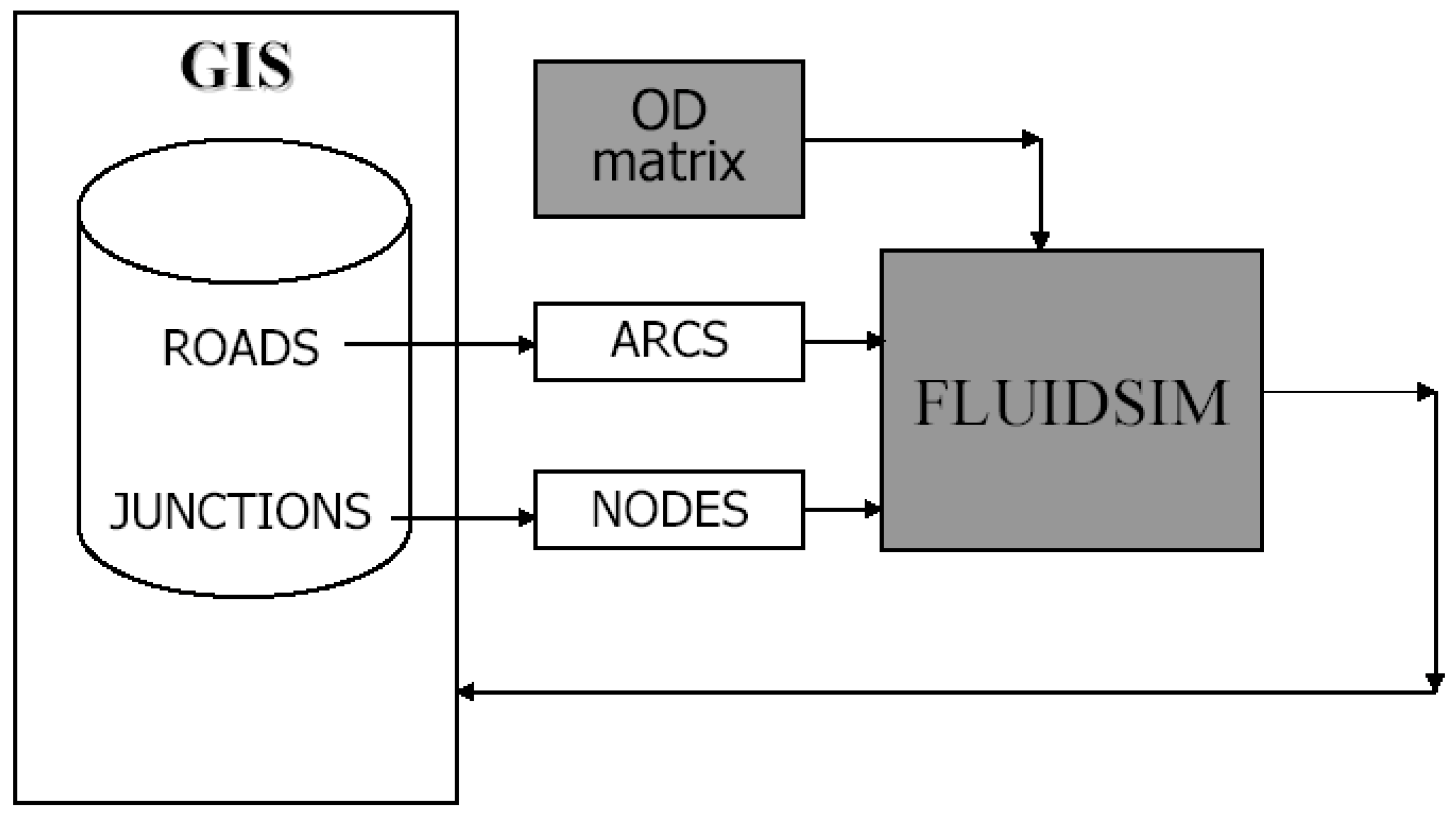
Figure 1. Architecture of the FLUIDSIM prototype.

Figure 1. Architecture of the FLUIDSIM prototype.

Node processing As reported in Section 2.2, each time the node processing routine is invoked, a LP problem must be solved at the optimum in order to produce the assignment for flows and density at the extreme points of the incident links interval. The linear programming formulation is quite concise, being in most cases the number of its variables and constraints equal to the number of roads incident to junctions. In general, the worst case is O(|E|) for both the number of variables and the number of constraints. In a first version of the prototype the node processing routine invoked an external mathematical solver [27], but due to the high number of times this routine must be run, the code was improved by embedding a simplex routine inside the code. The relevance of the computational time saving provided by this additional feature was tested, and the results are presented in Section 4.

Arc processing The arc processing routine computes, for each arc, a new density value for each segment in which an arc is divided by the numerical segmentation scheme, that is $\lfloor \frac{l_i}{\Delta s}\rfloor$. This is done by invoking each time the routines implementing the numerical approximation scheme. Depending on the size of Δs, on the number of arcs in the network, and on the choice of the scheme itself, this computation can represent the computational bottleneck of the system.

Software architecture In Figure 1, we provide a scheme of the prototype architecture. The core of the simulation environment is represented by the FLUIDSIM block, taking as an input the network structure, that can be exported from a Geographical Information System project as a file containing the list of nodes and links, together with a set of data concerning the initial state of density on arcs. The main output of the simulation at each time step is the profile of density values on arcs, that can be represented on a GIS system by means of the implementation of proper importation routines. In particular, varying accurately the density profile, if Δs is small enough, it could be interesting to visualize each arc segment differently on the map, instead of considering just the mean value for each arc. To this aim, dynamic segmentation can be used to consider all the discrete intervals in which each arc is divided when representing the map on a GIS.

Implementation details The prototype was implemented in ANSI C₊₊ language, and the code compiled with gcc on linux environment. Tests were performed on a single cpu Pentium 4 1.7GHz PC with 2Gb RAM.

Scalability properties The structure of the simulation algorithm suggests the possible use of grid computing and parallelization. In facts, at each iteration of the algorithm, the solutions at the junctions are computed by solving independently small linear programming maximization problems for each intersection n in N. The same holds for the Riemann problem solution: each arc can be processed separately from the others. Therefore, the availability of a cluster of CPUs or parallel processors can be exploited by implementing a version of the code directly tailored for the specific architecture, e.g., by exploiting multi-platform shared memory multiprocessing programming instruments, such the Open MPI application programming interfaces (API), in such a way to distribute the computational load on the different available processors during each iteration of the simulation.

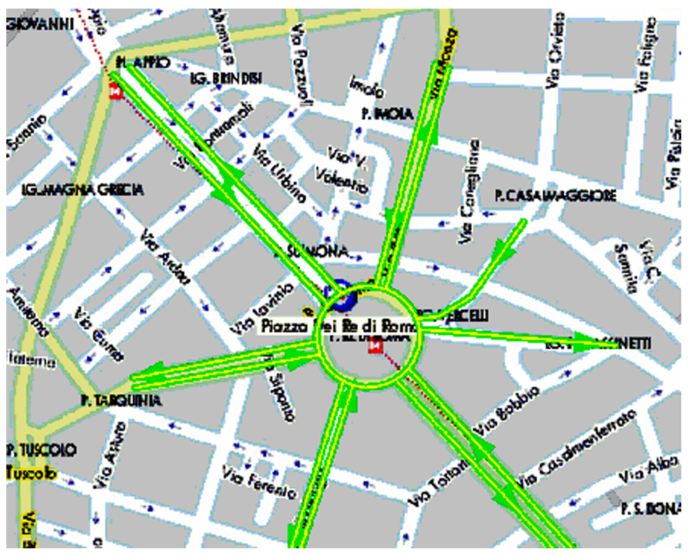
Figure 2. The extracted network used for the code test.

Figure 2. The extracted network used for the code test.

4. Computational Experience

In this section we present results of our computational tests in order to study the performance of this prototype and its suitability in the field of urban car traffic simulation networks. To this aim, we first analyze how computational times vary depending on some basic parameters. Then, we study the impact on the running time when an embedded simplex routine is used instead of invoking an external mathematical solver to solve flow conservation linear programming problems at nodes. Finally, we provide some results of case studies based on real networks.

4.1. Running time analysis

All the results presented in this section were conducted on a network formed by 24 roads and 12 junctions, as presented in Figure 2, representing a small area in the center of the City of Rome. All times are reported in seconds, and do not include the time needed for the exportation and the processing of the output data for successive visualization.

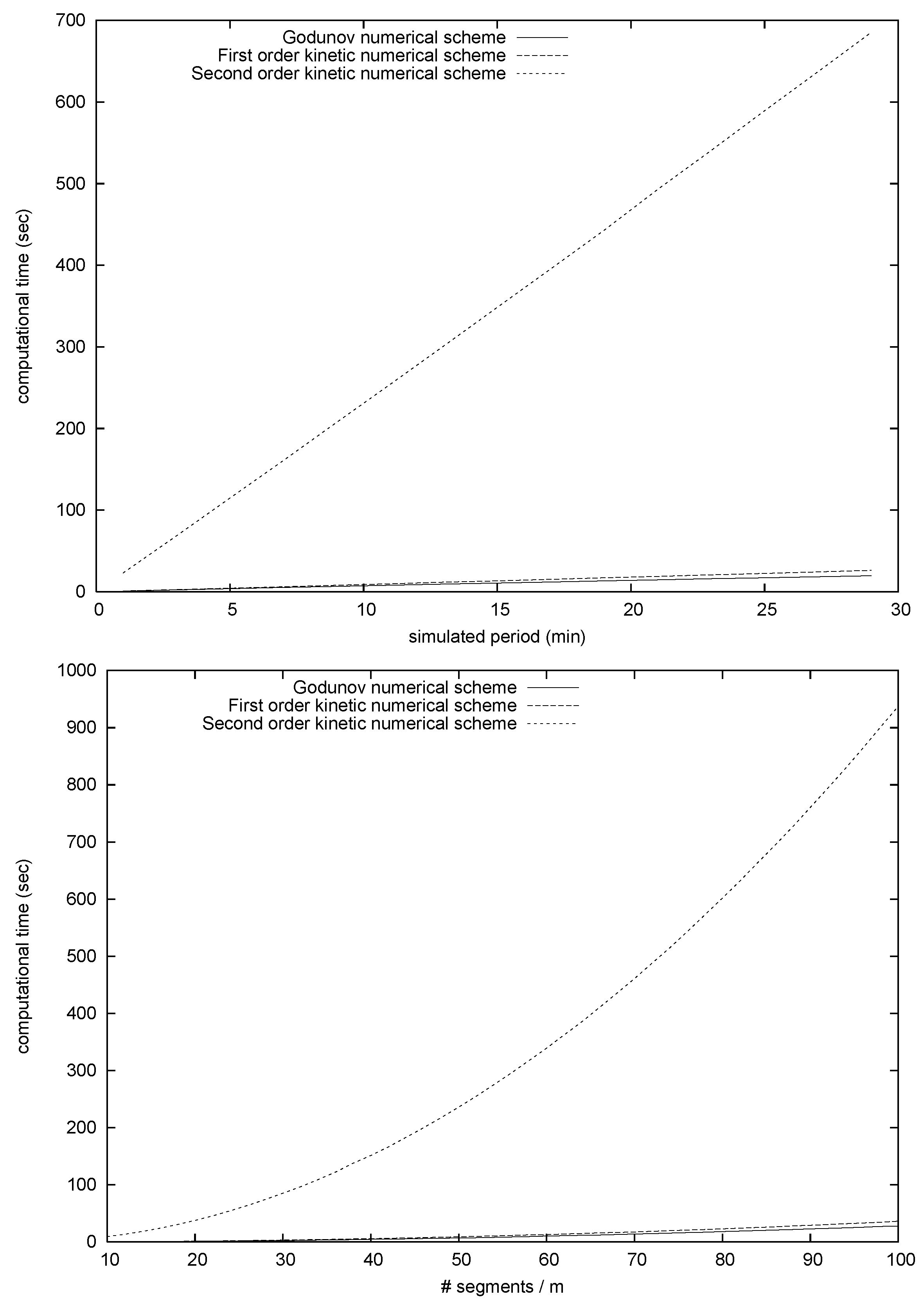
Figure 3. Comparing numerical approximation schemes: computational time (seconds) vs. simulated period (minutes) (top); computational time (seconds) vs. (number of segments)/meter (bottom).

Figure 3. Comparing numerical approximation schemes: computational time (seconds) vs. simulated period (minutes) (top); computational time (seconds) vs. (number of segments)/meter (bottom).

In Figure 3 (top), computational time is reported as a function of the simulated period. For 30 minutes simulations, the Godunov and the 1st order kinetic schemes require less that 60 seconds of computation, while the 2nd order scheme needs about 10 seconds for each minute of simulation. The balance between computational time and accuracy seems more convenient for first order schemes.

In Figure 3 (bottom), a similar analysis is presented considering the size Δs (which corresponds to the number of segments in which each road section is divided). Results confirm the strong computational effort required by the 2nd order approximation scheme. In particular the dependence on the Δs appear to be quadratic and no more linear as for the simulated period.

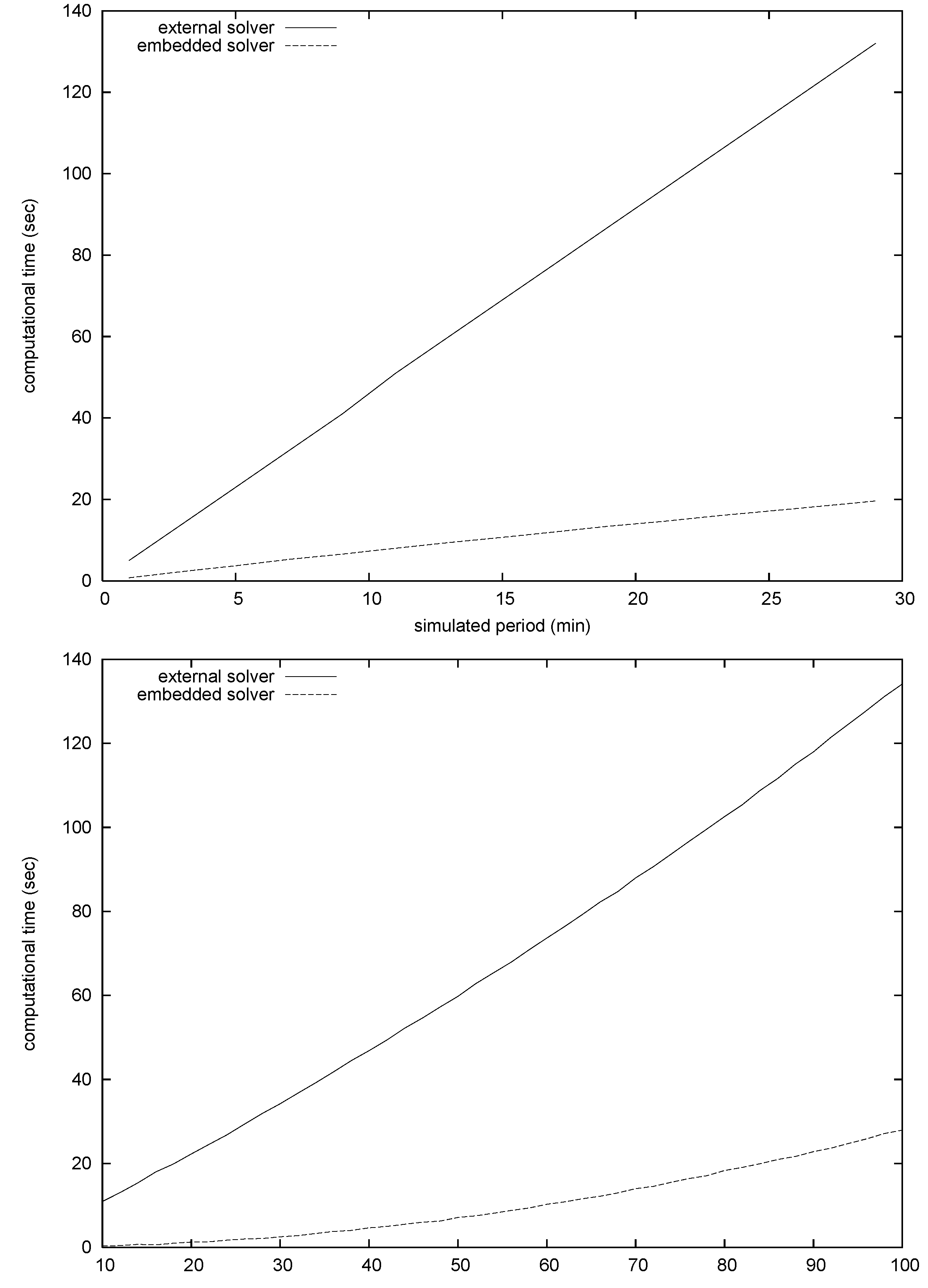
In Figure 4 the computational time profile is presented for the Godunov approximation scheme, comparing the performance obtained through the embedded simplex algorithm routine with respect to the use of the external LP solver. For this numerical scheme the efficiency gain is relevant, while the use of the 2nd order approximation scheme strongly reduces the impact of invoking an external solver, since in that case the computational bottleneck is in the arc processing routine.

Figure 4. Computational gain when embedding the PL solver algorithm in the code (Godunov numerical approximation scheme): computational time (seconds) vs simulated period (minutes) (top); computational time (seconds) vs (number of segments)/meter (bottom).

Figure 4. Computational gain when embedding the PL solver algorithm in the code (Godunov numerical approximation scheme): computational time (seconds) vs simulated period (minutes) (top); computational time (seconds) vs (number of segments)/meter (bottom).

4.2. Real networks case studies

Simulations were performed on real urban networks to test the suitability of this prototype in order to reproduce real traffic situations, and to test the scalability of the code on large size networks. In particular, the code was tested on the whole traffic network extracted from the city of Salerno, Italy, formed by about 1200 roads. GIS data of roads placement are courtesy of Salerno City Hall.

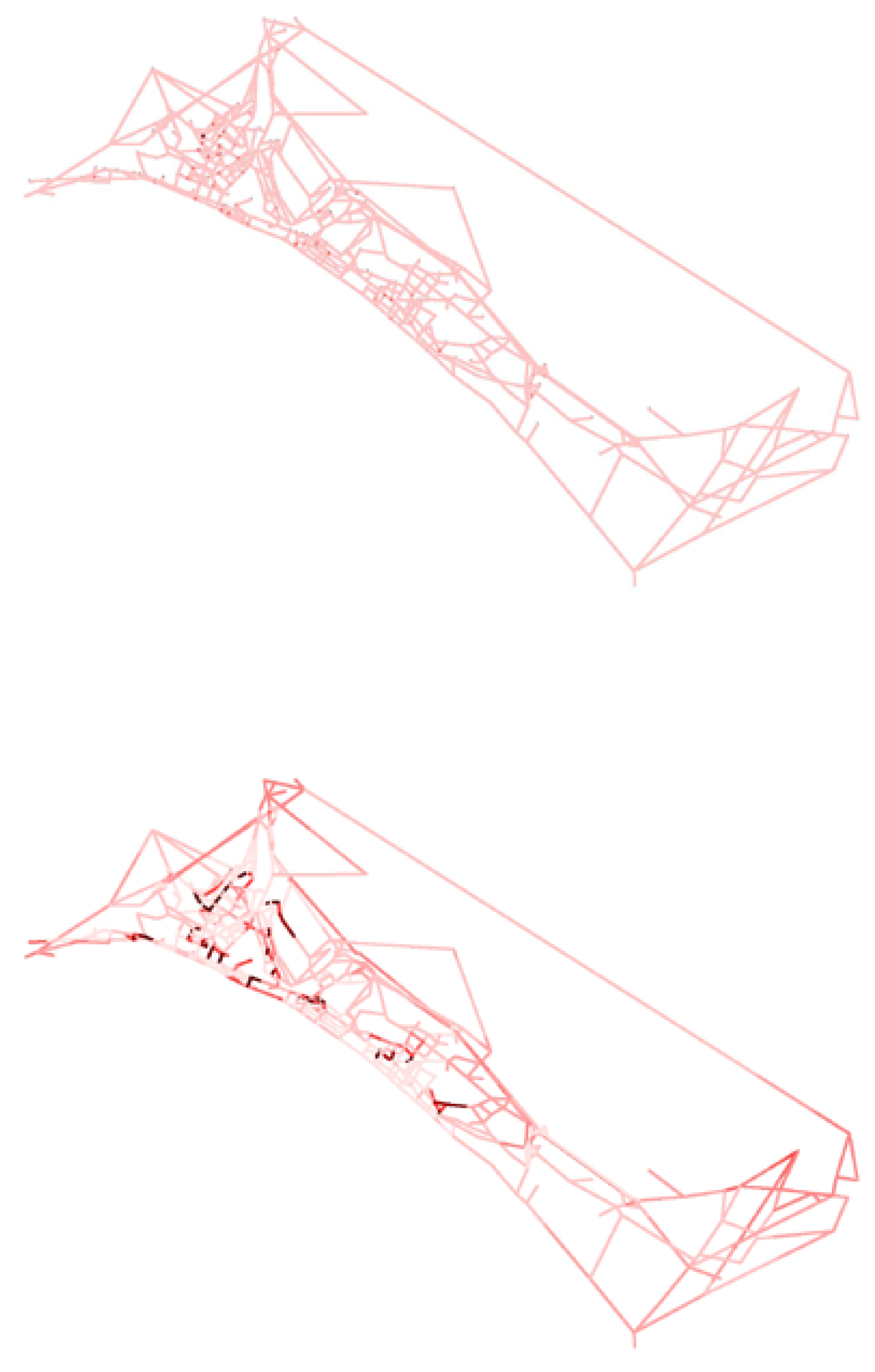
In Figure 5, we report the result of a 30 real minutes simulation. More precisely in Figure 5 (top) the load is reported at the beginning of the simulation. The load was artificially set to be low on every road, corresponding to 0.3 density. Arcs not connected to any node n in FS(n), i.e., as exiting road, are interpreted as sources from outside the network and a constant boundary datum of 0.3 density is assigned. Then the load evolves in the whole city, see Figure 5 (bottom) and higher densities are represented by darker red segments. It is possible to appreciate how the network structure of the whole city naturally gives rise to high density zones, where bottlenecks effects occur.

Figure 5. The full network of Salerno: before (top) and after (bottom) the simulation.

Figure 5. The full network of Salerno: before (top) and after (bottom) the simulation.

It is important to notice that such simulation has the meaning of illustrating the potentiality of the method, however one has to be cautious in deriving conclusions about the real traffic load have. Indeed, one should make use of real data to set the initial load. Also, source terms and absorption terms should be present due to parking lots, private and public sites, etc.

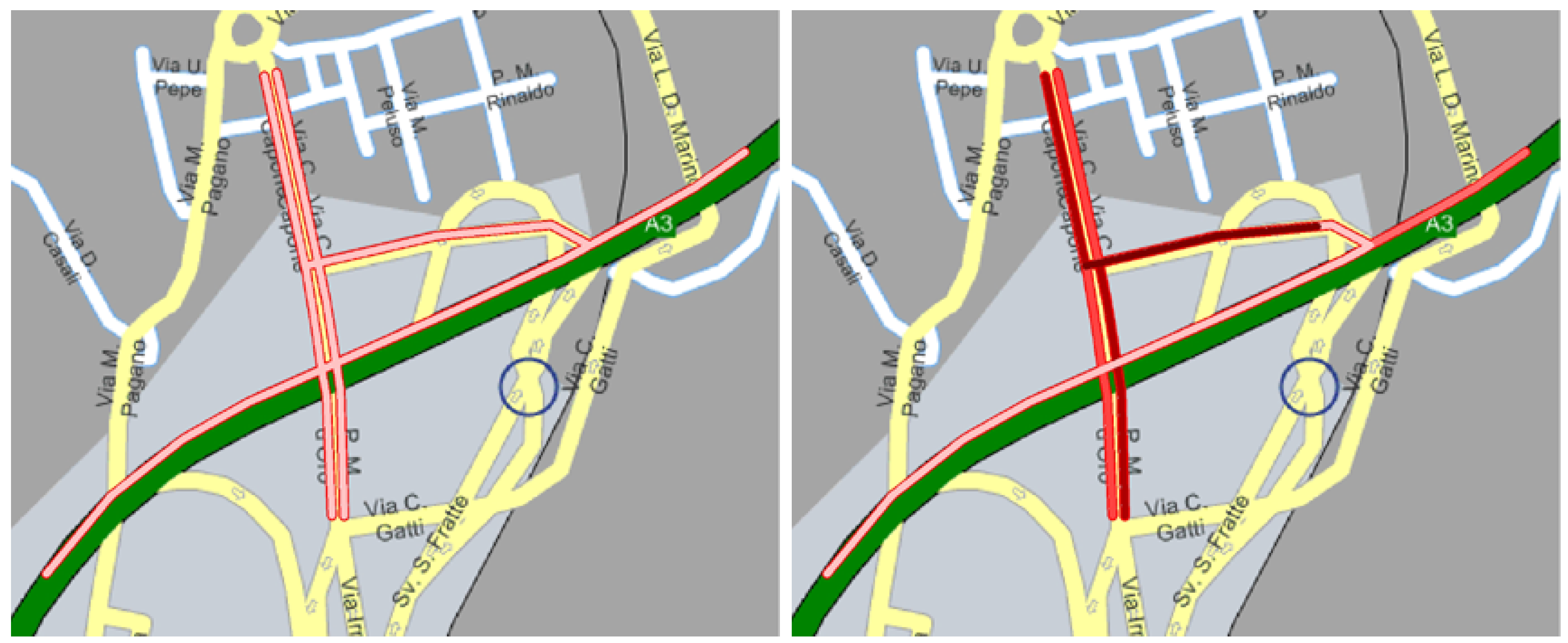
Then we focus on the junction of Salerno Fratte. At this crossing traffic exiting the highway A3, connecting Salerno to the Salerno Univerity area and the city of Avellino, meets that from the center city. Unfortunately, there is no priority for the traffic coming from the highway. As a result, long queues form at this junction and move backs into the highway. We report the simulation of this are in Figure 6. One can notice that the model well reproduce the real traffic behaviour. Also in this case dark red corresponds to high density.

Figure 6. A focus on a relevant junction: Salerno Fratte before (left) and after (right) the simulation).

Figure 6. A focus on a relevant junction: Salerno Fratte before (left) and after (right) the simulation).

Various other simulations were run with the present model and simulation prototype: Some movies can be downloaded from [28].