Alternatives to the Least Squares Solution to Peelle’s Pertinent Puzzle

Abstract
: Peelle's Pertinent Puzzle (PPP) was described in 1987 in the context of estimating fundamental parameters that arise in nuclear interaction experiments. In PPP, generalized least squares (GLS) parameter estimates fell outside the range of the data, which has raised concerns that GLS is somehow flawed and has led to suggested alternatives to GLS estimators. However, there have been no corresponding performance comparisons among methods, and one suggested approach involving simulated data realizations is statistically incomplete. Here we provide performance comparisons among estimators, introduce approximate Bayesian computation (ABC) using density estimation applied to simulated data realizations to produce an alternative to the incomplete approach, complete the incompletely specified approach, and show that estimation error in the assumed covariance matrix cannot always be ignored.1. Introduction
Peelle's Pertinent Puzzle (PPP) was introduced in 1987 in the context of estimating fundamental parameters that arise in nuclear interaction experiments [1]. PPP is described briefly below and in more detail in [2]. When PPP occurs, generalized least squares (GLS) behaves reasonably under the model assumptions [2]. However, in PPP, GLS parameter estimates fall outside the range of the data, which has raised concerns that GLS is somehow flawed and has led to suggested alternatives to GLS estimators.
Others [1,3-9,12-15] have investigated alternatives to the GLS approach to PPP, but no numerical performance comparisons to other methods have been reported. And, one ad hoc approach involving simulated data realizations is statistically incomplete [8].
The following section includes additional background for PPP and the GLS approach. Section 3 discusses the ordinary sample mean as a perhaps naive alternative and shows that estimation error in the assumed covariance matrix cannot always be ignored. Sections 4 and 5 develop an alternative involving a modified form of approximate Bayesian computation (ABC). This ABC-based approach uses density estimation applied to realizations of simulated data that follow an error model appropriate for PPP and having various error distributions. Section 6 provides a second Bayesian alternative resulting from completion of the ad hoc approach by specifying a suitable prior probability density function (pdf). Section 7 is a summary.
2. Background
A situation that leads to PPP is as follows. Two experiments aim to estimate a physical constant μ. Experiment one produces a measurement y1, and experiment two produces y2. Measurements y1 and y2 arise by imperfect conversion of underlying measurements m1 and m2. Suppose m1 = μ + ∊R1 and m2 = μ + ∊R2 where ∊R1 is zero-mean random error in m1 and similarly for ∊R2. Burr et al. [2] prove that if y1 =m1 + ∊S and y2 = m2 + α∊S, where ∊S ∼ N(0, σS) and α is any positive scale factor other than 1, the covariance matrix Σ of (y1, y2) can lie in the PPP region in which the GLS estimate of μ lies outside the range of y1 and y2. And, Burr et al. [2] give an example for which this error model is appropriate.
Let Σ be the 2-by-2 symmetric covariance matrix for y1 and y2 with diagonal entries , , and off-diagonal entry σ12, which denote the variance of y1, the variance of y2, and the covariance of y1 and y2, respectively. For the case considered here and in Zhao and Perry [4]
If the three errors ∊R1, ∊R2, and ∊S have normal (Gaussian) distributions, then the joint pdf of (y1, y2) is also normal. If the three errors have non-normal distributions, then the joint pdf of (y1, y2) will not be normal and might be difficult to calculate analytically. Therefore, to handle non-normal distributions that might be difficult to calculate analytically, Sections 4 and 5 develop an estimator based on ABC. This ABC-based estimation can be applied with the error model just described resulting from the two experiments producing y1, y2 values with a covariance given by Equation 1, and can accommodate non-normal distributions.
It is well known that GLS applied to y1 and y2 results in the best linear unbiased estimate (BLUE) μ̂ of μ [16]. Here, “best” means minimum variance and unbiased means that on average (across hypothetical or real realizations of the same experiment), the estimate μ̂ will equal its true value μ. GLS properties are well known and are reviewed in [2]. The GLS estimate for μ arising from the generic model
GLS estimation is guaranteed to produce the BLUE even if the underlying data are not normal. However, if the data are not normal, then the minimum variance unbiased estimator is not necessarily linear in the data. Also, unbiased estimation is not necessarily superior to biased estimation [17].
The main alternative to GLS estimation in this context is estimation that uses the pdf. When viewed as a function of the unknown model parameters (μ in our case) conditional on the observed data (y1, y2 in our case), the pdf is referred to as the likelihood. The maximum likelihood (ML) estimate therefore of course depends on the pdf for the errors. For example, the normal distributions are replaced with lognormal distributions, the ML estimate will change. Because the ML approach makes strong use of the assumed error distributions, the ML estimate is sensitive to the assumed error distribution. The ML method has desirable properties, including asymptotically minimum variance as the sample size increases. However, in our example, the sample size is tiny (two), so asymptotic results for ML estimates are not relevant. It still is possible that an ML estimator will be better for non-normal data than GLS. In this paper, “better” is defined as the mean squared error (MSE) of the estimator, which is well known to satisfy MSE = variance + bias2. In some cases, biased estimators have lower MSE than unbiased estimators because the bias introduced is more than offset by a reduction in variance [17]. The other estimators considered here are two versions of Bayesian estimators, both of which rely on the likelihood as does ML.
3. Estimation error in Σ̂
In nearly all real situations, Σ is not known exactly, but must be estimated. Suppose the estimate Σ̂ = S, where S is the sample covariance matrix defined as (t denotes transpose) based on n pairs of y1, y2 values that are auxiliary data pairs separate from the y1 = 1.5 and y2 = 1.0 values. We will consider two examples.
Example 3.1
Assume that the distribution of (n − 1)S is Wishart with ν = n − 1 degrees of freedom, which is exactly true if the y1 and y2 pairs are bivariate normal, and approximately true for many other bivariate distributions [18]. Then the root mean squared error ( , where E denotes expected value) in estimating the true mean μ using GLS, is 0.46, 0.32, 0.27, 0.25, 0.23, and 0.22 for ν = 2, 3, 4, 5, 10, and 30, respectively. These RMSE estimates are based on 10,000 simulations in R [19] and are repeatable to ±0.01. And the RMSE is 0.27 using the simple mean of y1 and y2. Recall that if Σ is known exactly, then the RMSE in μ̂ = 0.22. Therefore, if n ≤ 5, the naive sample mean has the same or lower RMSE than does GLS.
A third estimation option suggested in [20] uses only the variances of Σ̂, not because y1 and y2 are thought to be independent, but because the estimated covariance is thought to be unreliable. For ν = 2, 3, 4, 5, 10, and 30, option 3 has an RMSE of 0.25, which is the theoretical best RMSE corresponding to the situation in which σ1 and σ2 are known exactly. Therefore, there is merit in Schmelling's [20] suggested option 3 in this case, because it has lower RMSE for all values of ν than the simple mean and lower RMSE than GLS for small ν values. Whether option 1 (GLS), option 2 (naive sample mean), or option 3 (use variances only, not covariance) is preferred depends on the true data likelihood and on the true Σ.
Example 3.2
Still assuming a normal likelihood but changing , , and in Σ to 0.1134, 0.02, and 0.0475, respectively (cor(y1, y2) = 0.997), options 1, 2, and 3 have RMSE of 0.025, 0.24, and 0.17, respectively, for ν = 3, and 0.04, 0.24, and 0.17, respectively, for ν = 2. This Σ corresponds to a very strong PPP effect with high correlation between y1 and y2, so even with large estimation error in Σ̂, the GLS method has by far the lowest RMSE for all values of ν. We note that as ν → ∞, the GL μ̂ has σμ̂ → 0.017. As another example, let , , and in Σ be 0.1134, 0.0104, and 0.02, respectively. Then options 1, 2, and 3 have RMSE of 0.13, 0.20, and 0.12, respectively, for ν = 3, and RMSE of 0.25, 0.20, and 0.13, respectively, for ν = 2. So in this case option 3 is again a good choice for small values of ν. We note that as ν → ∞, the GLS μ̂ has σμ̂ → 0.096.
4. Approximate Bayesian Computation
Bayesian analysis requires a prior probability p(θ) for the parameters θ, and a likelihood f(D|θ) for the data given the parameter values. The result is a posterior probability π(θ|D) ∝ f(D|θ)p(θ) for the parameters θ. For many priors and likelihoods, calculating the posterior is difficult or impossible, but observations from the posterior can be obtained by Markov chain Monte Carlo (MCMC). MCMC is a Monte Carlo sampling scheme that accepts a candidate value θ′ with probability that depends on the relative probability of the current θ value and the candidate θ′ value. The goal of MCMC is to simulate many observations from the posterior, and use summary statistics such as posterior means and standard deviations to characterize the state of knowledge about the parameters. In our examples, θ is the scalar-valued mean which we denote throughout as μ.
ABC has arisen relatively recently in applications for which the likelihood f(D|θ) is intractable [22,23], but data can be simulated somehow, often relying on detailed simulations of physical processes. In our context, the simulation is very simple, based on realizations of the measurement error pdfs. And if some subset of the three underlying error distributions described in the background section are non-normal, leading to a complicated bivariate distribution for y1, y2 that could be difficult to derive analytically, then ABC is attractive. Predating ABC is a nonBayesian (“frequentist”) method referred to as “inference for implicit statistical models” [21,24] that was based on density estimation. We use the term ABC to include any Bayesian method in a situation for which an analytical likelihood is not available, but simulations can produce realizations from the likelihood.
In the common version of ABC, because data can be simulated from the pdf, candidate values θ′ can be accepted with a probability that depends on how close certain summary statistics such as the first few moments computed from the simulated data having parameter value θ′ are to the corresponding summary statistics from the real data. Some sources [24] reserve the term ABC for methods that rely on such summary statistics, so would not use the term ABC with density estimation. Our combination of MCMC with density estimation appears to be a new combination of ideas, though some might not refer to it as ABC. Regardless of the jargon, the method will be clearly delineated below.
As a simple example to motivate our modified form of ABC, suppose y1, y2, …, yn are independently and identically distributed as N(μ, σ) and it is known that σ = 0.1. Introductory statistics texts usually prove that the sample mean y̅ is the ML estimator (MLE) for μ and more advanced texts investigate properties of MLEs. And, Equation (3) with a diagonal Σ (because in this example the yi are independent) can be used to show that y̅ is the GLS estimator so is also the BLUE and because the data is normal in this simple example (but not in our extended PPP examples below), y̅ is also the MVUE. Specify the prior p(μ) to be . Then, because the normal prior for μ is the “conjugate” prior (meaning that the posterior distribution is the same type of distribution as the prior distribution) for the normal likelihood, the posterior π(θ|D) is , where .
Our modified ABC that relies on density estimation has the following steps:
Determine a lower (L) and upper bound (U) for the parameter μ. In this example, having observed y1, y2, …, yn1 and knowing σ = 0.1, we can assume μ lies between say L = y̅ − 5σ/n1 and U = y̅ + 5σ/n1.
Choose μ values on a grid of equally-spaced values in the range (L, U). For each μi value in the grid, simulate n2 observations from N(μi, σ) and use these n2 observations to estimate the pdf using density estimation [25]. In the toy example, we know the true pdf is N(μ, σ), but in cases below, we might not know the pdf because it involves algebraic combinations of non-normal pdfs.
The likelihood of each observed yj can be estimated by interpolation of the estimated pdf for each μi value in the grid. The size of the steps in the μ grid can be decreased and n2 can be increased until estimates of μ stabilize.
The overall likelihood is then the product (because the yj are independent) of the estimated likelihood for each observed yj
Use MCMC to estimate the posterior probability for μ, and to compute μ̂ as the mean of the posterior. To implement MCMC, we used the metrop function in the mcmc package in R and used the approx function to interpolate the estimated pdf on the grid of trial μ values. The Appendix has this “likelihood” function, where the estimated pdf is used in place of an analytical likelihood.
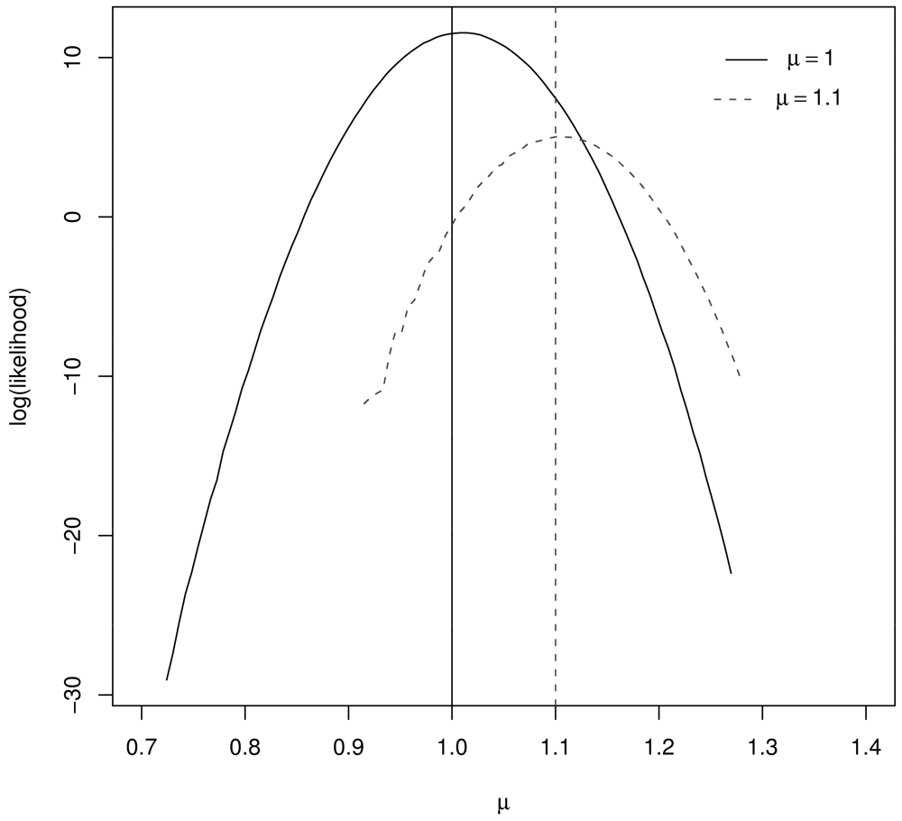
Figure 1 illustrates the resulting log likelihood for μ = 1, μ = 1.1, n1 = 10, and n2 = 1000. Notice that the log likelihood peaks very near the true μ value in both cases.
To check our implementation, we specified the prior p(μ) to be . Then, because the normal prior for μ is the “conjugate” prior (meaning that the posterior distribution is the same type of distribution as the prior distribution) for the normal likelihood, the posterior π(θ|D) is . The ABC estimate of the posterior mean can then be compared to the mean of the exact posterior π(θ|D) to ensure proper implementation. In this case, our implementation of ABC also leads to μ̂ ≈ y̅ because we used σ = 0.1, σprior = 10, and n1 = 10, so the posterior distribution has mean essentially equal to y̅. Specifically, in 100 simulations of the entire process of generating n1 = 10 observations, and applying density estimation to estimate the likelihood using n2 = 1000 observations resulted in no statistical difference (based on a paired t-test) between the 100 values of the exact Bayesian μ̂, the ABC estimate of μ̂, and μ̂ = y̅. Readers can duplicate our results using the R functions listed in the Appendix.
To our knowledge, this simple use of density estimation to substitute for having an analytical form for the likelihood has not been studied in the ABC literature. However, provided the data can be simulated sufficiently fast to acquire many observations (n2 = 1000 was sufficiently large in this toy problem), and provided the dimension of the data is not too large, density estimation is feasible and effective. In the PPP case, we have only two variables, y1 and y2, so certainly 2-dimensional density estimation is feasible. We note here that summary statistics such as moments from the real and simulated data in the MCMC accept/reject steps in typical ABC implementations are fast to compute, but convergence criteria and measures of adequacy are still being developed [23].
5. ABC for PPP
This section again uses the slightly modified form of ABC that relies on density estimation rather than using summary statistics computed from the real and simulated data, but MCMC is applied in the context of PPP.
As mentioned in Section 2, suppose from two experiments m1 = μ + ∊R1 and m2 = μ + ∊R2, where ∊R1 is zero-mean random error in m1 and similarly for ∊R2. Then if y1 = m1 + ∊S and y2 = m2 + α∊S, where ∊S ∼ N(0, σS) and α is any positive scale factor other than 1, the covariance matrix Σ of (y1, y2) can lie in the PPP region [2].
To implement our version of ABC, many (y1, y2) realizations are simulated from each of many values of μ Given the observed (y1, y2) and its known covariance Σ, we can again set up good L and U values for the grid of candidate μ values.
A key advantage of ABC is that any probability distribution can be easily accommodated for any of ∊R1, ∊R2, and ∊S. Here are two examples.
Example 5.1.
Assume ∊R1, ∊R2, and ∊S are all normal, so that y1, y2 is bivariate normal. Then as it must, our version of ABC recovers the GLS estimate μ̂ = 0.89.
Example 5.2.
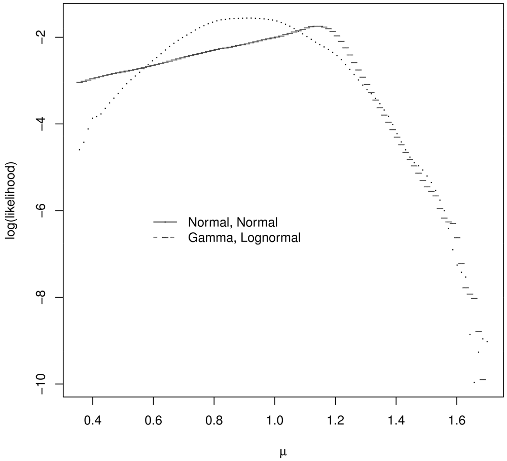
Assume ∊R1 and ∊R2 each have a centered and scaled lognormal distribution and ∊S has a centered and scaled gamma distribution, with parameters chosen so that the covariance matrix Σ of y1, y2 is given by Equation 1. Figure 2 plots the log likelihood for μ values in the μ grid for the correct (true) likelihood for y1, y2 and assuming a bivariate normal distribution for y1, y2. These log likelihoods are meaningfully different and one might expect the corresponding estimators to behave quite differently. For the single realization of y1, y2 = 1.08, 1.24, for which Figure 2 was generated, the GLS and ABC estimate assuming a bivariate normal distribution for y1, y2 is 1.27. The ABC estimate assuming the correct bivariate distribution for y1, y2 is 1.03.
To investigate whether using the correct likelihood leads to smaller RMSE, we performed 100 simulations for various values of μ in this same example 5.2. In each simulation, one new (y1, y2) pair was generated to represent the observed data pair, and then 10,000 observations of (y1, y2) pairs were generated to use for density estimation so that the likelihood of each candidate value of μ could be approximated. For example, with μ = 1.0, the RMSE for GLS is 0.22 as expected, and the RMSE for ABC using the correct bivariate distribution is 0.15 (repeatable across sets of 100 simulations to ±0.01). So, ABC has smaller RMSE than GLS in this case. However, ABC relies much more strongly on the estimated likelihood which relies on the assumed data distributions, so is not expected to be as robust to misspecifying the likelihood as GLS.
Recall that μ̂ via GLS is always outside the range of (y1, y2) when PPP occurs, and that some researchers are bothered by this. For the non-normal data just described, even though PPP occurs, we find numerically that μ̂ via ABC sometimes lies outside the range of (y1, y2) and sometimes lies within the range of (y1, y2).
6. Alternate Bayesian Approach to Complete the Ad hoc Approach
Reference [8] presented an ad hoc procedure to estimate μ as follows.
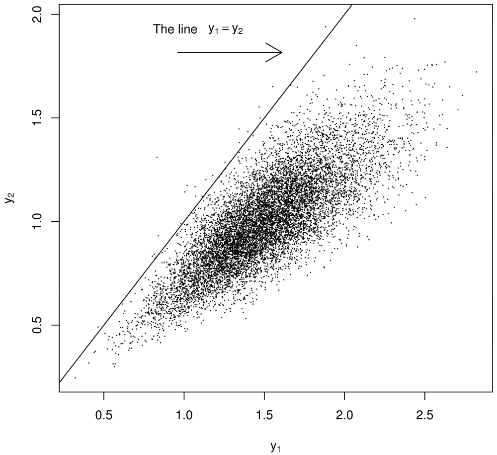
Using a model of the two experiments that produce y1, y2 such as that by [4] in Section 2, generate thousands of a y1, y2 pairs but regard them as being μ1, μ2 pairs. See below for “justification” in switching from y1, y2 to μ1, μ2. Because of the strong prior belief that μ1 ≈ μ2, restrict attention to bivariate points (y1, y2) lying very near the diagonal, defining μ̂ as the value that maximizes the estimated probability density of the scalar-values of either y1 or y2 (or both y1 and y2) satisfying |y1 − y2| < ∊ for some small ∊ near 0. See Figure 3. As an important aside, recall [2] showed that PPP cannot occur with this error model (Section 2). However, because of how Σ is estimated (using m1 or m2 to estimate μm), PPP appears to occur with this error model.
In one dimension, the analogous ad hoc procedure for a sample of size n from a normal distribution, is to assume μ ∼ N(y̅, σ2/n) in the case of unknown μ and known variance σ2 with . The formally correct posterior for μ depends on the likelihood and on the prior, but for a normal likelihood y ∼ N(μ, σ2) and a normal prior μ ∼ N(μp, τ2), as the prior variance τ2 → ∞, the prior becomes “flat,” and the ad hoc procedure is well known to be correct in an asymptotic sense.
Although this ad hoc approach in two dimensions is a recipe that can be followed to produce μ̂, it is statistically incomplete. It can be completed and justified by adopting a two dimensional prior for μ. That is, to regard y1, y2 pairs as being μ1, μ2 pairs requires that y1, y2 pairs be interpreted as being observations from the posterior distribution for μ1, μ2 in a Bayesian sense. Second, to formalize the notion of restricting attention to bivariate points (μ1, μ2) lying very near the diagonal, we must define a prior probability distribution. Specifically, assume
Let the prior for μ in Equation 5 be
The recipe to restrict attention to simulated values satisfying y1 ≈ y2 is ad hoc, but for a given choice of ∊ to define y1 ≈ y2 as satisfying |y1 − y2| < ∊, there is a defensible Bayesian posterior corresponding to a choice for Σprior. And, given
For example, choosing
This Bayesian approach revises the ad hoc recipe and is easily implemented using MCMC for any likelihood. It is sometimes difficult to calculate the likelihood for complicated combinations of distributions involving for example sums and products of random variables (which can arise in modifications of the prescription to generate y1, y2 pairs). An appeal of the modified ad hoc approach is that the likelihood does not need to be computed. Instead, one need only be able to generate many y1, y2 pairs. This is the same appeal of the ABC approach in our context.
To summarize this section, the ad hoc approach in [8] regards simulated (y1, y2) pairs from any distribution as providing an estimate of μ by specifying a small ∊ and computing the mean of all scalar-valued y1 and y2 satisfying |y1 − y2| < ∊ (or by finding the value of μ that maximizes the likelihood of the scalar data that arise from concatenating all y1 and y2 values that are similar). This approach has a corresponding formally correct Bayesian interpretation, but is easier to implement than the corresponding correct Bayesian implementation with a particular choice of the prior pdf.
For Example 5.1 in Section 5, for which the distributions for ∊R1, ∊R2, and ∊S are normal, the estimates arising from the Bayesian posterior maximum probability and the posterior mean are 0.89 and 0.89, respectively, both the same as the GLS estimate.
Example 6.1.
If the distributions for ∊R1, ∊R2, and for ∊S are centered and scaled product normals, the estimates for all small values of ∊ (∊ less than approximately 0.01) are 1.10 and 1.09, respectively from the Bayesian posterior maximum probability and the posterior mean.
If the distributions for ∊R1, ∊R2 are centered and scaled product normal and the distribution for ∊S is a centered and scaled gamma, the estimates for all small values of ∊ are 1.33 and 1.18, from the Bayesian posterior maximum probability and the posterior mean, respectively.
The fact that the estimates can lie between y1 and y2 appeals in some way.
Example 6.2
The ad hoc method can be formally defended by the Bayesian framework just described. Therefore, the ad hoc approach is included among the candidates whose RMSEs were given in Example 5.2 from Section 5. In the second part of Example 5.2, there are 100 simulations of 10,000 observations of (y1, y2) pairs (for which the RMSE of GLS and ABC are 0.22 and 0.15, respectively). The the RMSE of the ad hoc approach is 0.24 (repeatable to within ±0.01).
For Example 6.2, although the RMSEs from low to high (low is good) are ABC, GLS, and alternate Bayes, for this example, we do not make any general performance claims ranking GLS, ABC, and the modified ad hoc (“alternate Bayes”) approaches. Instead, the goal is to present statistically defensible approaches and demonstrate that they do perform differently.
Figure 4 illustrates the ad hoc and revised procedures in the case of the normal distribution. The top plot shows the accepted (μ1, μ2) pairs in the metrop MCMC (in red), which tightly follow the diagonal line. The bottom plot shows the estimated density of the accepted pairs using the Bayesian strategy and using the ad hoc strategy. Notice that the two densities are not the same. However, in this case, both methods arrive at μ̂ = 0.89 as the estimate for μ.
7. Conclusion
There will almost always be estimation error in Σ̂, and often the measurement errors are non-normal. Therefore, we considered the following three topics: (1) alternatives to GLS when there is estimation error in Σ̂, (2) approximate Bayesian computation [22] to provide estimators other than GLS that use the estimated likelihood in the case of non-normal error models that make ML estimation difficult, and (3) completion of an incompletely specified ad hoc approach to deal with non-normal likelihoods [8].
Regarding (1), it was illustrated in the PPP case that weighted estimates do not always outperform equally-weighted estimates when there is estimation error in the weights. We have already noted that estimation of Σ in Equation 1 introduces apparent PPP when PPP does not actually occur.
Regarding (2), ABC based on density estimation to estimate the required likelihood was introduced. We showed that for some likelihoods, Bayesian estimation can outperform GLS, and that for some data realizations, the ABC estimator fell within the range of the simulated x1, x2 data pairs. Of course GLS provides a good estimate μ̂ in general because of its well-known BLUE property (and UMVUE if the data is normal) and in particular for the PPP problem if the covariance Σ is well known.
Regarding (3), ad hoc estimators based on incomplete statistical reasoning did produce values that lie within the data range [8]. We modified the incomplete approach by another use of Bayesian reasoning that involved a two-component prior. We concur that for some data realizations, the ad hoc estimator can lie within the data range, but in the examples considered, the RMSE of this estimator was slightly higher than the RMSE of the GLS or ABC estimators.


Acknowledgments
We acknowledge the U.S. NNSA, and the Next Generation Safeguards Initiative (NGSI) within the U.S. Department of Energy.
Appendix
This appendix lists R functions.
Remark 1: The mcmc function in R, requires a log “likelihood” function.
Remark 2: Our ABC implementation uses the estimated pdf instead of an analytical likelihood.
mutrue = 1; sigma = .1
mu.grid = seq(mutrue-3*sigma,mutrue+3*sigma,length=100)
llik1 = numeric(length(mu.grid))
for(i in 1:length(mu.grid)) {
xtemp = rnorm(n=105,mean=mu.grid[i],sd=sigma)
temp.density = density(xtemp,n=1000)
llik1[i] = sum(log10(approx(temp.density$x,temp.density$y,xout=mu.grid)$y))
}
plot(mu.grid[5:95],llik1[5:95],xlab=expression(mu),ylab=”log(likelihood)”,type=”l”)
abline(v=1)
llik1.fun = function(mu,llik=llik1,mu.grid.use=mu.grid,prior.mean=0,prior.sd=10) {
llik.temp = approx(x=mu.grid.use,y=llik,xout=mu)$y
prior = log(dnorm(mu,mean=prior.mean,sd=prior.sd))
llik.temp = llik.temp + prior
if(is.na(llik.temp)) llik.temp = −1010
if(llik.temp == -Inf) llik.temp = −1010
llik.temp
}
library(mcmc) out1 = metrop(obj=llik1.fun,llik=llik1,initial=1,blen=10,scale=0.1,nbatch=1000)
plot(out1$batch) # basic diagnostic plot to check mcmc convergence
mean(out1$batch) # Result: approximately 1.0, the correct answer.
#product normal case
llik2.fun = function(mu,llik=llik2,mu.grid.use=mu.grid,prior.mean=0,prior.sd=10) {
llik.temp = approx(x=mu.grid.use,y=llik,xout=mu)$y
prior = log(dgamma(mu,shape=prior.mean/prior.sd,rate=1/prior.sd)) # true mean is nonzero
llik.temp = llik.temp + prior
if(is.na(llik.temp))llik.temp = −1010
if(llik.temp == -Inf) llik.temp = −1010
llik.temp
}
x = c(1.5,1)
library(MASS) # kde2d for 2-dim kernel density estimation
mu.grid = seq(0.3,1.7,length=100)
n = 105 # observations from simulation for each value of mu in grid of mu values
llik5a = numeric(length(mu.grid))
nvar1 = 0.1134; nvar2 = 0.0504; ncov12 = 0.06
alpha = .7
svar = ncov12/alpha
rvar1 = nvar1 - svar
rvar2 = nvar2 - alpha2 * svar
for(i in 1:length(mu.grid))
mu = mu.grid[i]
tempS = svar.5 * rnorm(n) * rnorm(n)
x1temp = mu + tempS +rvar1.5 * rnorm(n) * rnorm(n)
x2temp = mu + alpha * tempS + rvar2.5 * rnorm(n) * rnorm(n)
temp.density = kde2d(x=x1temp,y=x2temp,lims=c(x[1],x[1],x[2],x[2]),n=1)
llik5a[i] = log(temp.density$z)
llik5a[llik5a==-Inf] = min(llik5a[llik5a != -Inf])
tempy = lokerns(x=mu.grid,y=llik5a,x.out=mu.grid)
llik5a = tempy$est
llik2[llik1a==-Inf] = min(llik2[llik2 != -Inf])
tempy = lokerns(x=mu.grid,y=llik1a,x.out=mu.grid)
llik2 = tempy$est
out2 = metrop(obj=llik2.fun,initial=1,llik=llik2,blen=10,scale=.3,nbatch=1000,prior.mean=1,prior.sd=1)
mean(out2$batch) # Result: approximately 0.89.
References
- Peelle, R. Peelle's Pertinent Puzzle; Oak Ridge National Laboratory: Oak Ridge, TN, USA, 1987. [Google Scholar]
- Burr, T.; Kawano, T.; Talou, P.; Hengartner, N.; Pan, P. Defense of the Least Squares Solution to Peelle's Pertinent Puzzle. Algorithms 2011, 4, 28–39. [Google Scholar]
- International Evaluation of Neutron Cross Section Standards; International Atomic Energy Agency: Vienna, Austria, 2007.
- Zhao, Z.; Perey, R. The Covariance Matrix of Derived Quantities and Their Combination; ORNL/TM-12106; Oak Ridge National Laboratory: Oak Ridge, TN, USA, 1992. [Google Scholar]
- Chiba, S.; Smith, D. A Suggested Procedure for Resolving an Anomaly in Least-Squares Data Analysis Known as Peelle's Pertinent Puzzle and the General Implications for Nuclear Data Evaluation; ANL/NDM-121; Argonne National Laboratory: Argonne, IL, USA, 1991. [Google Scholar]
- Chiba, S.; Smith, D. Some Comments on Peelle's Pertinent Puzzle. JAERI-M 94-068. Proceeding of Symptoms on Nuclear Data; Japan Atomic Energy Research Institute: Tokai, Japan, 1994; p. 5. [Google Scholar]
- Chiba, S.; Smith, D. Impacts of Data Transformation on Least-Squares Solutions and Their Significance in Data Analysis and Evaluation. J. Nucl. Sci. Technol. 1994, 31, 770–781. [Google Scholar]
- Hanson, K.; Kawano, T.; Talou, P. Probabilistic Interpretation of Peelle's Pertinent Puzzle. Proceeding of International Conference of Nuclear Data for Science and Technology, Santa Fe, NM, USA, 26 September–1 October 2004; Haight, R.C., Chadwick, M.B., Kawano, T., Talou, P., Eds.; American Institute of Physics: College Park, MD, USA, 2005. [Google Scholar]
- Sivia, D. Data Analysis—A Dialogue With The Data. In Advanced Mathematical and Computational Tools in Metrology VII; Ciarlini, P., Filipe, E., Forbes, A.B., Pavese, F., Perruchet, C., Siebert, B.R.L., Eds.; World Scientific Publishing Co.: Singapore, Singapore, 2006; pp. 108–118. [Google Scholar]
- Jones, C.; Finn, J.; Hengartner, N. Regression with Strongly Correlated Data. J. Multivar. Anal. 2008, 99, 2136–2153. [Google Scholar]
- Finn, J.; Jones, C.; Hengartner, N. Strong Nonlinear Correlations, Conditional Entropy, and Perfect Estimation, AIP Conference Proceedings 954; American Institute of Physics: College Park, MD, USA, 2007.
- Kawano, T.; Matsunobu, H.; Murata, T.; Zukeran, A.; Nakajima, Y.; Kawai, M.; Iwamoto, O.; Shibata, K.; Nakagawa, T.; Ohsawa, T.; Baba, M.; Yoshida, T. Simultaneous Evaluation of Fission Cross Sections of Uranium and Plutonium Isotopes for JENDL-3.3. J. Nucl. Sci. Technol. 2000, 37, 327–334. [Google Scholar]
- Kawano, T.; Hanson, K.; Talou, P.; Chadwick, M.; Frankle, S.; Little, R. Evaluation and Propagation of the Pu239 Fission Cross-Section Uncertainties Using a Monte Carlo Technique. Nucl. Sci. Eng. 2006, 153, 1–7. [Google Scholar]
- Oh, S. Monte Carlo Method for the Estimates in a Model Calculation. Proceedings of Korean Nuclear Society Conference, Yongpyung, Korea, october 2004.
- Oh, S.; Seo, C. Box-Cox Transformation for Resolving Peelle's Pertinent Puzzle in Curve Fitting; PHYSOR-2004; The Physics of Fuel Cycles and Advanced Nuclear Systems: Global Developments: Chicago, IL, USA; April 25–29; 2004. [Google Scholar]
- Christensen, R. Plane Answers to Complex Questions, The Theory of Linear Models; Springer: New York, NY, USA, 1999; pp. 23–25. [Google Scholar]
- Burr, T.; Frey, H. Biased Regression: The Case for Cautious Application. Techometrics 2005, 47, 284–296. [Google Scholar]
- Johnson, R.; Wichern, D. Applied Multivariate Statistical Analysis; Prentice Hall: Upper Saddle River, NJ, USA, 1988. [Google Scholar]
- R Foundation for Statistical Computing. R: A Language and Environment for Statistical Coputing. 2004. Avalable online: www.R-project.org (accessed on 17 June 2011). [Google Scholar]
- Schmelling, M. Averaging Correlated Data. Phys. Scr. 1995, 51, 676–679. [Google Scholar]
- Diggle, P.; Gratton, R. Monte Carlo Methods of Inference for Implicit Statistical Models. J. R. Stat. Soc. B 1984, 46, 193–227. [Google Scholar]
- Marjoram, P.; Molitor, J.; Plagnol, V.; Tavare, S. Markov Chain Monte Carlo Without Likelihoods. Proc. Nat. Acad. Sci. USA 2003, 100, 15324–15328. [Google Scholar]
- Plagnol, V.; Tavare, S. Approximate Bayesian Computation and MCMC. Proceedings of Monte Carlo and Quasi-Monte Carlo Methods; National University of Singapore: Singapore, Singapore, 2002; pp. 99–114. [Google Scholar]
- Blum, M. Approximate Bayesian Computation: A Nonparametric Perspective. J. Am. Stat. Assoc. 2010, 105, 1178–1187. [Google Scholar]
- Hastie, T.; Tibshirani, R.; Friedman, J. The Elements of Statistical Learning; Springer: New York, NY, USA, 2001. [Google Scholar]
© 2011 by the authors; licensee MDPI, Basel, Switzerland. This article is an open access article distributed under the terms and conditions of the Creative Commons Attribution license (http://creativecommons.org/licenses/by/3.0/).
Share and Cite
Burr, T.; Graves, T.; Hengartner, N.; Kawano, T.; Pan, F.; Talou, P. Alternatives to the Least Squares Solution to Peelle’s Pertinent Puzzle. Algorithms 2011, 4, 115-130. https://doi.org/10.3390/a4020115
Burr T, Graves T, Hengartner N, Kawano T, Pan F, Talou P. Alternatives to the Least Squares Solution to Peelle’s Pertinent Puzzle. Algorithms. 2011; 4(2):115-130. https://doi.org/10.3390/a4020115
Chicago/Turabian StyleBurr, Tom, Todd Graves, Nicolas Hengartner, Toshihiko Kawano, Feng Pan, and Patrick Talou. 2011. "Alternatives to the Least Squares Solution to Peelle’s Pertinent Puzzle" Algorithms 4, no. 2: 115-130. https://doi.org/10.3390/a4020115