Radio-Frequency Interference Detection and Mitigation Algorithms for Synthetic Aperture Radiometers

 ,
,
Abstract
: The European Space Agency (ESA) successfully launched the Soil Moisture and Ocean Salinity (SMOS) mission in November 2, 2009. SMOS uses a new type of instrument, a synthetic aperture radiometer named MIRAS that provides full-polarimetric multi-angular L-band brightness temperatures, from which regular and global maps of Sea Surface Salinity (SSS) and Soil Moisture (SM) are generated. Although SMOS operates in a restricted band (1400–1427 MHz), radio-frequency interference (RFI) appears in SMOS imagery in many areas of the world, and it is an important issue to be addressed for quality SSS and SM retrievals. The impact on SMOS imagery of a sinusoidal RFI source is reviewed, and the problem is illustrated with actual RFI encountered by SMOS. Two RFI detection and mitigation algorithms are developed (dual-polarization and full-polarimetric modes), the performance of the second one has been quantitatively evaluated in terms of probability of detection and false alarm (using a synthetic test scene), and results presented using real dual-polarization and full-polarimetric SMOS imagery. Finally, a statistical analysis of more than 13,000 L1b snap-shots is presented and discussed.1. Introduction
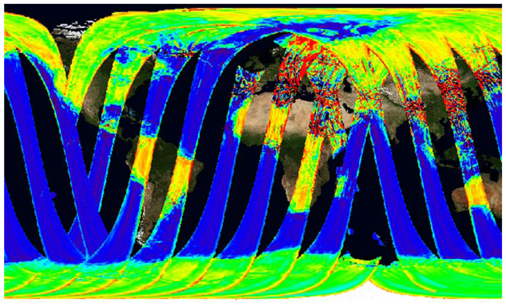
The European Space Agency (ESA) mission “Soil Moisture and Ocean Salinity” (SMOS) was successfully launched on November the 2, 2009. Its main objectives are the determination of Soil Moisture (SM) over land [1] and Sea Surface Salinity (SSS) over the oceans [2], with an accuracy of 0.04 m3/m3 every three days with a spatial resolution of 50 km [3] (R-4.6.1–002 to 004) at level 2, and 0.1 psu every 10 days with a spatial resolution of 200 km [3] (G-4.7.2–005) at level 3. Unfortunately, the first SMOS images [4] using calibration data from the on-ground Image Validation Tests showed a large amount of radio-frequency interference (RFI), specially over land in Europe and Asia, but in some small areas of Africa and Greenland as well (Figure 1).
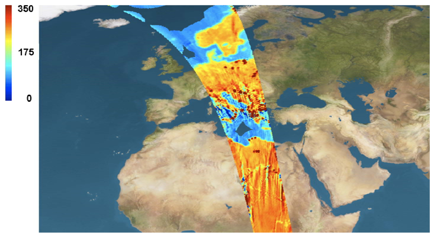
A refined analysis using on-board calibration data allowed to “focus” the brightness temperature images (i.e., get sharper details). However, even though RFI regions became more localized, the amount of RFI was on many occasions so large that the tails of the “impulse response” of a quasi-point RFI source (see Figures 15b and 21) extended over the whole image, hampering the retrieval of geophysical parameters, mainly over land, but not exclusively (Figure 2).
In [6], a theoretical study of the impact of RFI in SMOS demonstrated that, when the measured normalized cross-correlations (μ) among all pairs of signals collected by the interferometric radiometer array are small, for a sinusoidal RFI source in the (ξi, ηi) = (sin θi·cos Φi, sin θi·sin Φi) direction, and power , the error is approximately a correlation offset given by:
An analysis of the potential sources of RFI and their impact was also performed [6], including:
nearby emissions from L-band radars, non-GSO (non Geo-Stationary Orbit) and GSO MSS (Geo-Stationary Orbit Mobile Satellite Services),
harmonics of lower frequency emissions, and
possible jamming, which may or may not be deliberately generated. Table 1 from [6] summarizes the potential interferences from nearby emissions and harmonics that can affect an L-band synthetic aperture radiometer.
From all possible interferences, the most important ones were predicted to be those generated by:
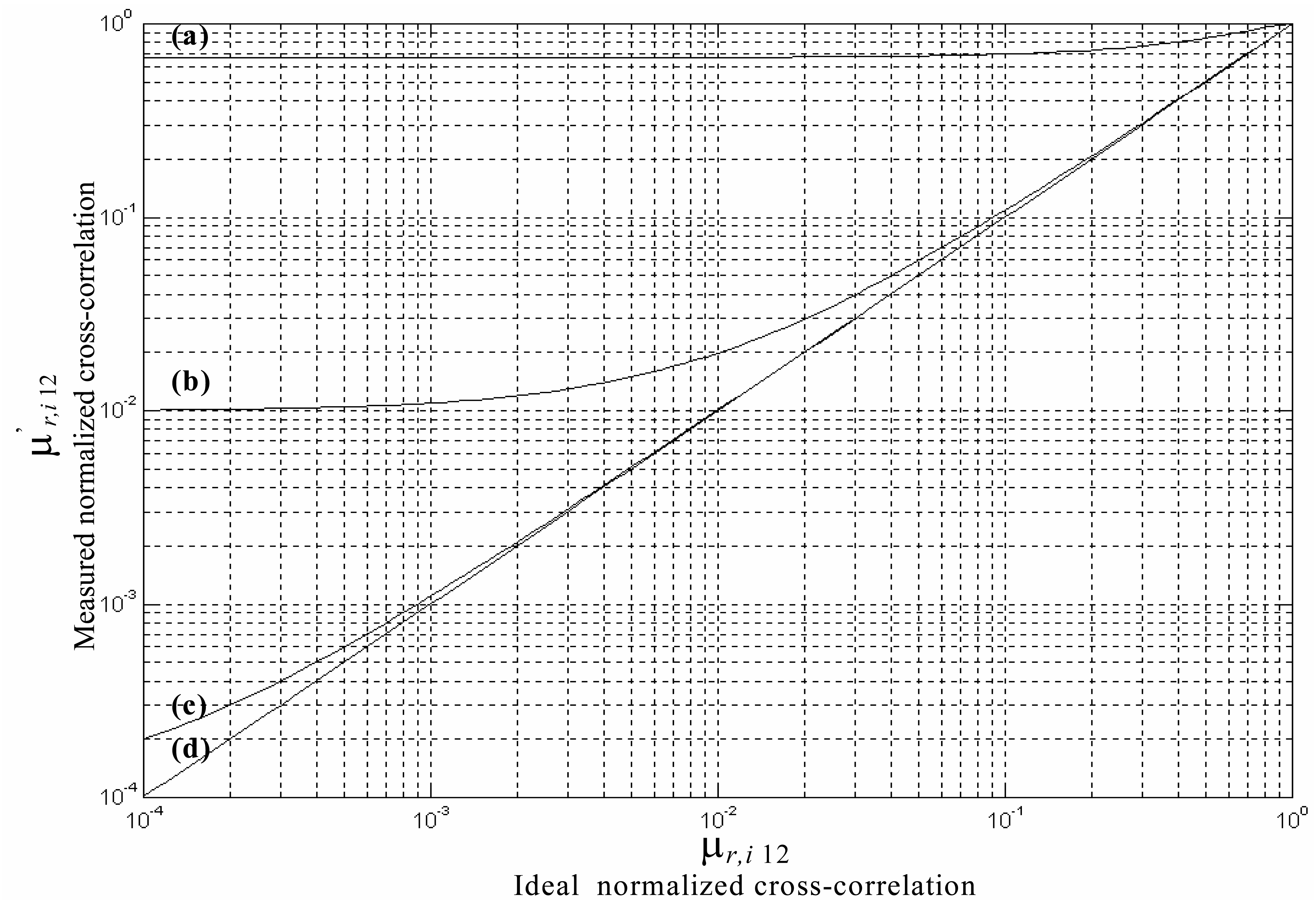
L-band radars due to the high levels of transmitted power, which may interfere in an area as large as 80 km × 700 km (cross-track × along-track), for an error level of eμ≥ 10−2 (see Figure 4), and
non-GSO MSS up-link transmitters (due to the low spurious rejection and their proximity to the 1400-1427 MHz band), which may interfere in an area of 50 km × 92 km (cross-track × along-track), for an error level of eμ≥ 10−2. This behavior was confirmed by SMOS imagery, showing artifacts as North-South stripes (Figure 2).
However, 10 years after this study [6] was conducted, SMOS is now suffering also from RFI generated by the ubiquitous use of wireless devices such as surveillance video cameras, WIFI networks etc. which can create out-of-band emissions if their outputs are not properly filtered, and even in some cases, emissions within the protected band.
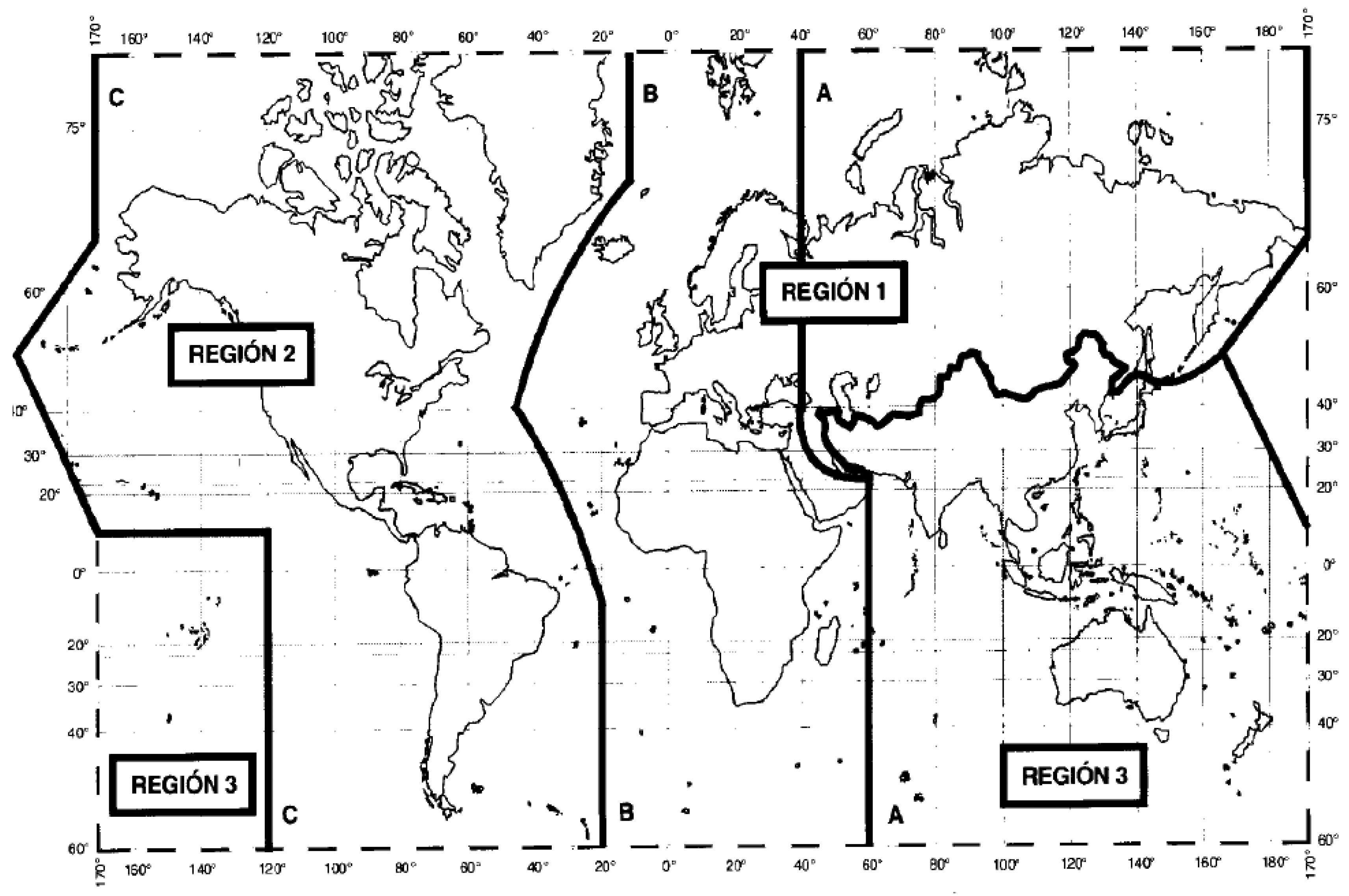
Figure 5 shows the world radio-electric spectrum division in three regions [8]. The fact that Europe is one of the regions most affected by RFI, while Regions 2 and 3 (except China, and conflictive zones) are generally clean (Figure 6), seems to indicate that fixed and mobile services (assigned in this band too, but only in Region 1), may be more important than radio-localization services (assigned in all three Regions) [8,9]. Figure 6 shows also the important effect that law enforcement can have in the quality of the data over large areas. For example, a strong RFI source in the center of Spain was turned off on March 16 thanks to the efforts of the Dirección General de Telecomunicaciones (belonging to the Ministerio de Fomento, Spain), CDTI (Centro para el Desarrollo Tecnologico e Industrial), INSA (Ingenieria y Servicios Aerospaciales), and ESA (European Space Agency).
In Section 2, a number of typical RFI scenarios are first presented to understand the nature of RFI, and the constraints the RFI detection and mitigation algorithms must face. In Section 3, a RFI detection and mitigation algorithm implemented to operate directly on L1b SMOS dual-polarization or full-polarimetric data is described. Finally, Section 4 presents the statistical analysis performed on more than 13,000 snap-shots.
2. Understanding the Impact of RFI in Synthetic Aperture Microwave Radiometry Imagery
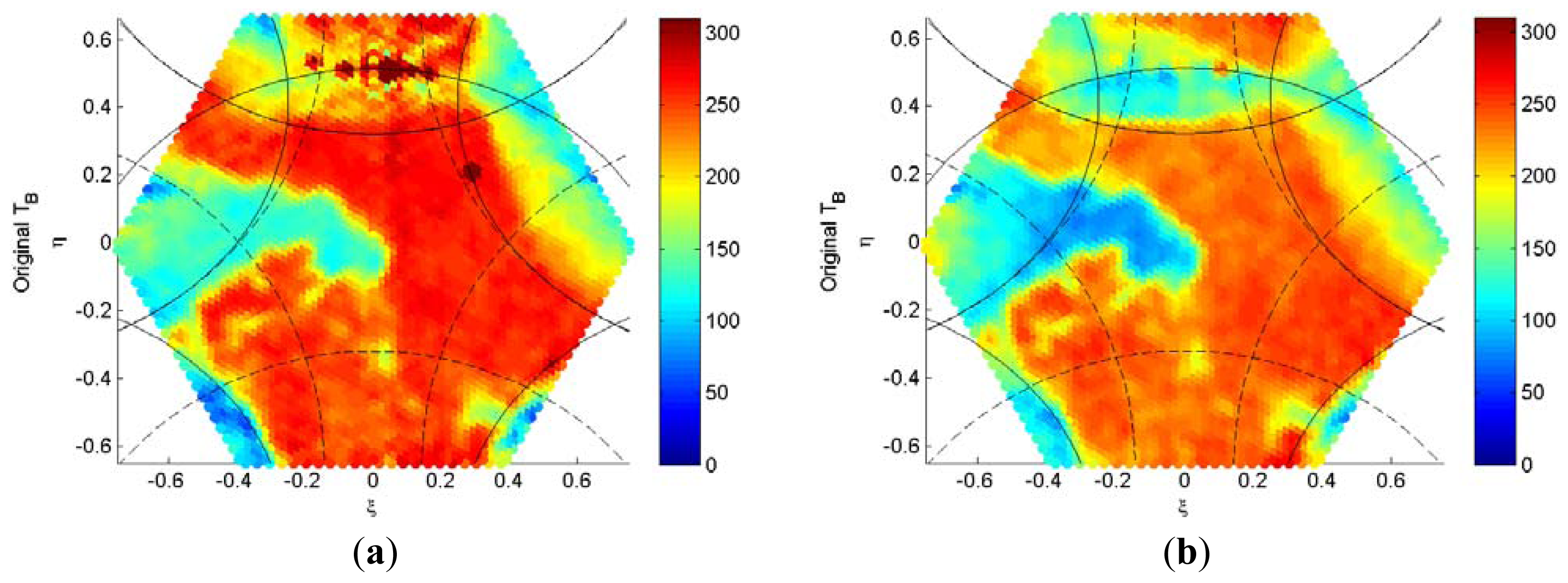
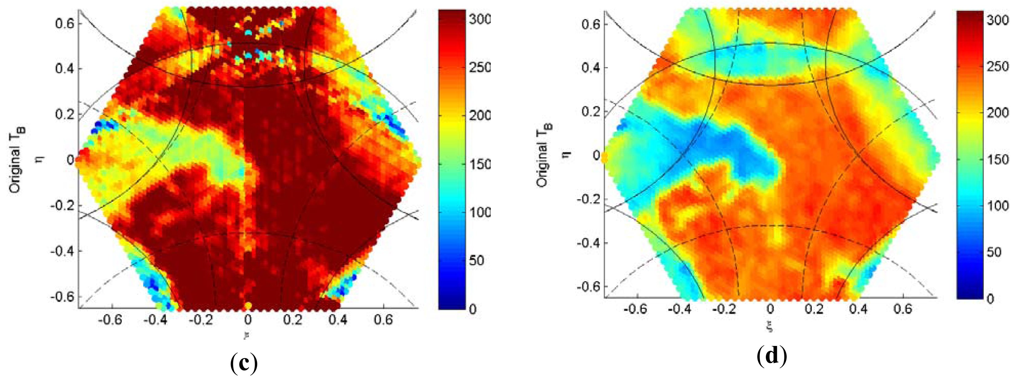
Figures 7 to 10 show different SMOS L1b imagery corresponding to different RFI scenarios on March 3, 2010. In these figures, the hexagon in the (ξ, η) domain corresponds to the full hexagonal period in which the synthetic image is formed by a kind of Fourier synthesis process from the (u, v) visibility samples (cross-correlations from the signals collected by pairs of antennas) acquired over a hexagonal grid determined by the characteristic Y-array of the MIRAS instrument aboard the SMOS mission [7]. In the imaging process, replicas (“aliases”) of the unit circle (ξ2 + η2 = 1, all directions in front of the array) appear centered at a distance 2·λ/(√3·d) from the origin, being d the spacing between consecutive antennas in the array. Since in MIRAS/SMOS d = 0.875 λ, aliases are centered at 1.32 ≤ 2 and overlap with the main image (centered at 0) restricting the instrument's alias-free field-of-view (FOV) [11]. In Figures 7 to 10, the dashed lines correspond to the unit circle and its aliases, and the solid lines to the Earth-sky horizon and its aliases.
Plots (a) and (c) correspond to Y-polarization, while (b) and (d) to X-polarization, acquired sequentially every 1.2 s in dual-polarization mode. Figures 7 to 9 show a typical behavior in which RFI sources appear in the Earth-sky horizon (over the solid lines) and have a very well defined polarization characteristics: RFI sources are stronger at Y-polarization, than they are at X-polarization, which in this part of the FOV approximately correspond to the vertical and horizontal polarizations, respectively. It is worth noting that they are very variable with time (see Figures 8a vs. 8c, and Figure 9a vs. 9c, and to less extent Figures 9b vs. 9d). In some cases (Figure 9c) RFI is so strong that it completely corrupts the whole brightness temperature (BT) image, not only appearing as a strong point source, but eventually corrupting the denormalization coefficients of the visibility samples as well and corrupting the whole image. Figure 10 shows a snap-shot around the Caspian Sea with strong RFI sources, but most of them are in the alias regions.
As a consequence, it can be concluded that:
Since RFI sources are usually very time-dependent and polarization-dependent as well, RFI detection and mitigation algorithms must operate on a snap-shot basis only, independently for each polarization. Averaging of RFI estimates from different snap-shots as a way to improve the estimated RFI power is, therefore, not possible; and
Since most RFI sources appear in the alias regions, but their impact extends over the “alias-free” FOV, RFI detection and mitigation algorithms must operate in the whole hexagonal period.
3. RFI Detection and Mitigation Algorithm in Synthetic Aperture Microwave Radiometry Imagery
Before describing the proposed RFI detection and mitigation algorithm, it is important to understand the two basic modes of operation of the MIRAS instrument aboard SMOS:
Dual-polarization mode: antenna switches sequentially connect all the receivers to the X-polarization antenna probe or to Y-polarization antenna probe (one receiver per dual-polarization antenna element), obtaining a BT image at X- or Y-polarization in one switching interval (1.2 s). This mode of operation corresponds to the SMOS images processed corresponding to March 3, 2010.
Full-polarimetric mode: the antenna switches connect the receivers in one array arm either to the X- or Y-polarization antenna probes following a predetermined sequence. Figures 11 and 12 adapted from [12] show these sequences. What is important in this mode is that the four Stokes parameters images are obtained after four switching intervals, and due to the pulsed nature of many RFI sources (e.g., pulsed and/or rotating radars…) RFI can happen in one of the intervals, and not in the others, in an unpredictable manner. In the SMOS imagery, the effects are subtle, since in the main beam a “hot” spot appears, but the side lobes and tails of the impulse response are distorted, and fictitious third and fourth Stokes parameters appear. This mode of operation corresponds to the images processed from September 3, 2010.
For these reasons, two different algorithms have had to be developed, one for each mode of operation.
3.1. Dual-Polarization Mode Algorithm
As can be appreciated in Figures 7 to 10, most RFI sources appear as point sources to instrument's angular resolution. Therefore, they look like the MIRAS instrument impulse response, even though in many cases their amplitude is not strong enough so that the tails of the impulse response (see Figures 15b and 21) appear clearly differentiated from the BT background.
The proposed algorithm takes advantage of previous techniques developed in the frame of the SMOS mission, such as the successful Sun cancellation algorithm [13] and the extended CLEAN [14]. The steps of the algorithm are summarized below:
Very strong RFI sources:
- 1.
If the BT of a large fraction (user-selectable) of pixels is larger than a given threshold—The 350 K threshold is selected to be above the maximum brightness temperature of a blackbody at the maximum temperature registered on the Earth (∼58 °C = 331 K). Sun glint is not an issue, because it always happens on Earth's pixels outside the extended alias-free field of view—(e.g., 350 K), the whole snap-shot is flagged as totally contaminated (see Figure 8c).
Strong RFI sources: if the snap-shot is not flagged as totally contaminated then:
- 2.
BT pixels larger than a given threshold (e.g., 350 K) are flagged as potentially corrupted.
- 3.
Following the same concept of the Sun cancellation algorithm derived in [13], but applied recursively as in the CLEAN algorithm [14] to all the BT pixels found in step #2, the strongest RFI sources are located and recursively cancelled. In this way, not only the main lobe of the impulse response is attenuated (eventually cancelled), but the side lobes as well. In this case the main problems are that:
As opposed to the Sun, the exact location of the RFI sources is not a priori known, and the accuracy of the estimation is limited by the step of the (ξ, η) grid. In the SMOS data processing ground segment the grid size is 128 × 128 pixels. In the proposed algorithm an optimum interpolation based on hexagonal Fourier transforms [11] and zero-padding is performed to try to determine more precisely the position of the sources (up to 4 times thinner grid).
Due to the (usually) lower values of the equivalent BT values of the RFI sources, as compared to the Sun (between 105 and 106 K), the background BT estimation becomes more critical (Equations 11–16 in [13]),
Background BT estimation is even more difficult, since most RFI sources tend to be in coastal regions where population concentrates. This means that about half of the surrounding pixels are land pixels, and about half are sea pixels. And
Since RFI sources tend to be very time-dependent, it is not possible to average a number of consecutive snap-shots to improve the RFI amplitude estimations.
Moderate RFI sources: in the remaining BT image, once strong sources have been cancelled or attenuated (mitigated, but not totally cancelled),
- 4.
A background image is subtracted. This background BT image is computed from the BT image resulting from step #3, but low-pass filtered with a disk of 6 pixels radius.
- 5.
In the differential image (step #4: cleaned BT image minus background image), pixels with values larger than N·ΔT(ξ, η) are flagged as RFI and not as noise spikes. The user-defined factor N is selected in such a way that the noise spikes characterized by the radiometric sensitivity ΔT(ξ, η) at a given pixel (ξ, η) in the BT image have a low probability of occurrence. In our case N is set to 3, then the probability that BT(ξ, η) > background + 3·ΔT (ξ, η) is equal to:
This probability is basically the probability of false alarm (Pfa) associated to noise spikes (Pfa = 0.13%). In a non-uniform background situation, spikes may appear in strong BT gradients, which will increase Pfa.
- 6.
The modified Sun cancellation algorithm (step #3) only works for circular or quasi-circular RFI sources (shape of the impulse response) and not for extended RFI sources such as those that can be found, for example, in large metropolitan areas. The criterion to define whether a region detected in step #5 is a quasi-circular region is the following:
- 7.
Ideally, bound1 and bound2 should be 1, since only circles satisfy that 4·π·area/perimeter2 = 1. However, due to discretization effects in the (ξ, η) grid it has been empirically found that many RFI sources are properly cancelled if the bounds are extended up to bound 1 = 0.2, and bound 2 = 4.
- 8.
For regions satisfying step #5 and #6, the procedure explained in step #3 is applied.
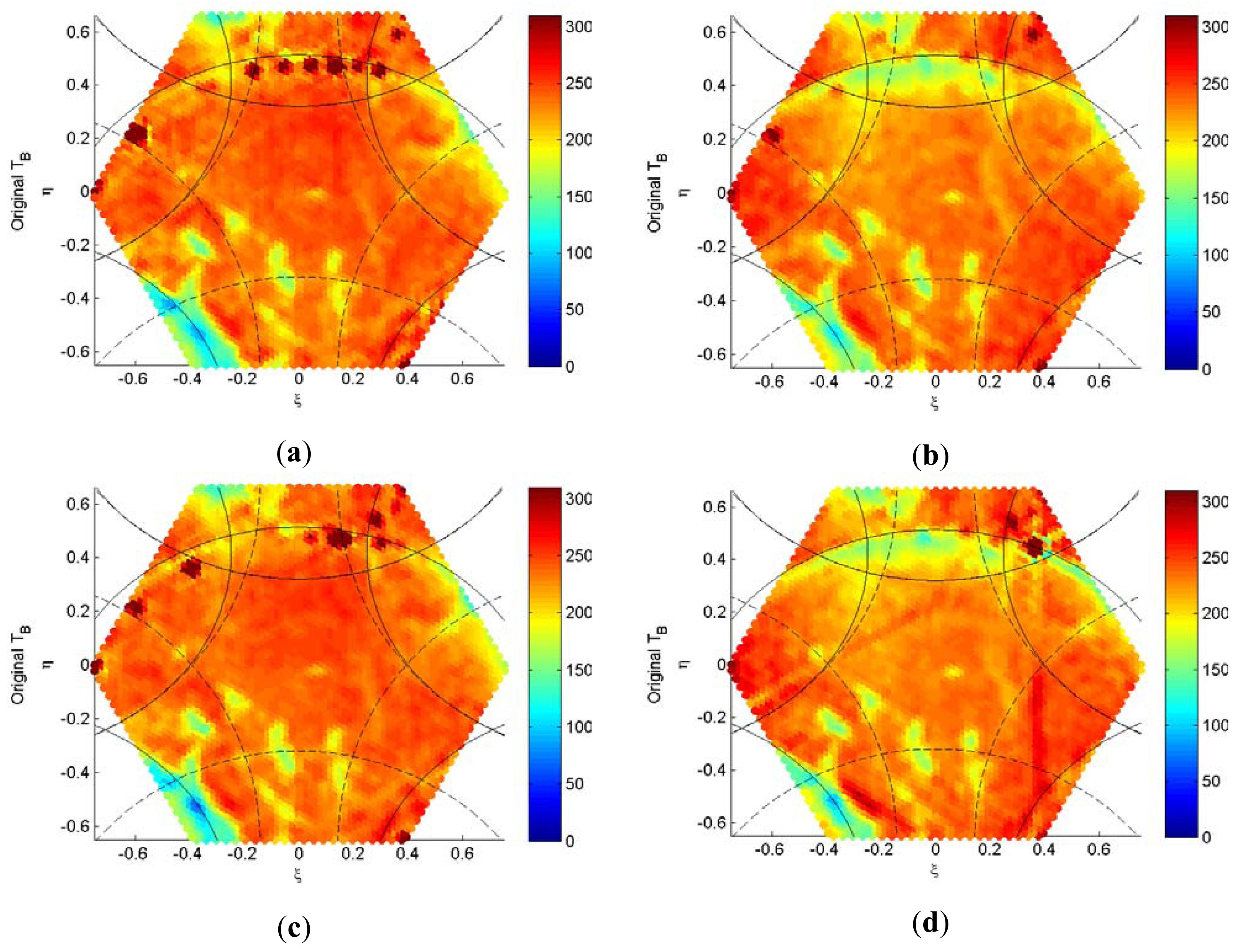
The performance of this algorithm is qualitative shown with real SMOS data in Figures 13 and 14, corresponding to Figures 9 and 10. It works reasonably well for most quasi-point sources, even if they are in the alias regions. On some occasions it tends to over-compensate the RFI sources, while on others it fails to compensate them completely due to errors in the location of the sources and/or estimation of the background. One of the drawbacks is that it cannot handle extended targets as the ones in Figure 13c, even though they are not too extended. The algorithm explained in Section 3.2 shows how to handle such cases.
3.2. Full-Polarimetric Mode Algorithm
At the end of the SMOS commissioning phase it was decided that the instrument should operate in full-polarimetric mode only. In this mode of operation the four Stokes parameters images (TXX, TYY, Real{TXY} and Im{TXY} are obtained after four switching intervals, as sketched in Figure 11. In many cases, pulsed RFI sources happen in one or several of the intervals, but not in all with the same amplitude, which distorts the side lobes and tails of the impulse response, preventing the use of the Sun cancellation algorithm described in Section 3.1. Also, since they affect only a subset of the whole visibility samples, fictitious third and fourth Stokes parameters may appear.
In order to better understand the differences of the problem in the full-polarimetric case, as compared to the dual-polarization one (section 3.1), Figure 15 illustrates these effects with an SMOS image acquired on September 3, 2010 over the Aegean Sea (Cyprus island appears in the bottom part of the image).
As can be appreciated in the TXX image (Figure 15a,b), there is an intense RFI source around (-0.25, +0.35) whose “tails” (impulse response) are not even symmetrical: the tails at +30° and at -90° with respect to the ξ axis are mostly negative (dark blue color), instead of positive, indicating that this RFI source has occurred only during some intervals of the switching sequence. The other RFI sources, being even stronger (e.g., (-0.35, -0.02) and (0.19, -0.35)) appear more “round” and symmetric, indicating that the RFI was most probably present during the four switching periods. Figures 15c and 15d show the TYY image. Compared to Figure 15a, the strongest sources are now in different positions, new ones can also be seen, while others have nearly disappeared, particularly the one at (-0.25, +0.35). Figures 15e and 15f show the real and imaginary parts of TXY (Re[TXY] and Im[TXY]) in the alias-free FOV, which should be close to zero in the Earth horizontal-vertical reference frame (Re[THV] and Im[THV]), but actually are not. This reveals the presence of new RFI sources that have passed inadvertently in the TXX and TYY images.
The fact that Re[TXY] and Im[TXY] should be close to zero is based on two factors:
the low cross-polar antenna pattern in the alias-free FOV, and
the fact that the third and fourth Stokes parameters in the Earth's reference frame are negligible (if not zero for most surface covers).
Outside the alias-free FOV, the values of Re[TXY] and Im[TXY] increase due to the overlapping of regions far away from the antenna boresight, where the co- to cross-polar ratio is much lower. Figures 16a and 16b show the mean values of Re[TXY] and Im[TXY] computed over the ocean to minimize the risk of undetected RFI.
Note also that, within the alias-free field of view, the TXX(ξ, η) and TYY(ξ, η) images (Figure 16a,b) capture the angular dependence of the brightness temperatures at X- and Y-polarizations in the antenna reference frame, which allows easily distinguishing RFI contaminated pixels. Over land, the problem is more complex due to the large range of BTs that can be encountered.
At this moment, two strategies can be followed:
to use only the YY- and XX-polarization BT images obtained during the time intervals 0-τ and 2·τ-3·τ, respectively (marked as 1 and 1′ in Figure 11), and use the dual-polarization RFI detection and mitigation algorithm (Section 3.1). This approach throws away half of the data (time intervals τ-2·τ and 3·τ-4·τ) and would not make any use of the polarimetric information contained in Re[TXY] and Im[TXY], which can be very helpful in detecting the presence of RFI.
to define a set of new different masks to detect the presence of RFI in the BT image at XX- or YY-polarization images in the full-polarimetric mode using all the available information. This process is described below:
BT pixels (XX- or YY- polarizations) larger than a given threshold (threshold 1, e.g., 350 K1) are flagged as corrupted (Figure 17a). This is equivalent to step #2 in the dual-polarization algorithm.
A background image computed from the original BT image low-pass filtered with a disk of 6 pixels radius is subtracted from the original image. The pixels whose value is larger than another threshold (threshold 2, e.g., 350 K1, as well) and that correspond to the land part only of the BT image are flagged as corrupted (Figure 17b).
A third mask is computed from those pixels in |Re[TXY(ξ, η)]| that differ from the mean |Re[TXY(ξ, η)]| image (Figure 16c) more than a given threshold (threshold 3, e.g., 250 K, larger than the maximum expected |Re[TXY(ξ, η)]| values). These pixels are flagged as corrupted (Figure 17c).
A fourth mask is computed from those pixels in |Im[TXY(ξ, η)]| that differ from the mean |Im[TXY(ξ, η)]| image (Figure 16d) more than a given threshold (threshold 4, e.g., 50 K). These pixels are flagged as corrupted (Figure 17d).
Finally, a fifth mask is computed for the ocean pixels only for which TXX(ξ, η) or TYY(ξ, η) differ from the mean TXX(ξ, η) or TYY(ξ, η) images (Figures 16a or 16b) more than N·ΔT(ξ, η) are flagged as corrupted (Figure 17e). In the algorithm described N is set to 3, and ΔT(ξ, η) is the radiometric sensitivity in the (ξ, η) direction, as explained in Section 3.1.
The global mask used for RFI detection is actually the “or” of the five previous masks, that is, a pixel is flagged, if RFI is detected in any of the tests. Land and ocean pixels are differentiated to take into account their different angular signature, as shown in Figure 17f with light blue the ocean (and sky) pixels, and in maroon, the land pixels that are susceptible to being contaminated by RFI.
Now, for the RFI mitigation, ocean and land pixels have to be treated in a differentiated manner, that is, a land-sea mask is needed. For the ocean pixels, the corrupted pixels are replaced by their corresponding mean ones (Figure 16a or 16b). For the land pixels an interpolation method based on an object removal and exemplar-based region filling is used, which combines the best texture synthesis with inpainting algorithms [15]. In addition, this technique produces a confidence map to indicate the reliability of the interpolated values: from 0 (not reliable at all) to 1 (totally reliable). Actually, this interpolation technique could also be used for the ocean pixels as well, but in many cases (i.e., Figure 18 below) the number of corrupted pixels in the whole image is so large, that the algorithm does not function. Therefore, we have resorted to use the mean values over the corrupted ocean pixels, and then interpolate only the contaminated land pixels.
Figures 18, 19 and 20 show three different examples of the application of the RFI detection and mitigation algorithm described above for the real SMOS data in full-polarimetric case. Figure 18 corresponds to a SMOS image over the Aegean Sea acquired on September 3, 2010 (a few snap-shots earlier than that in Figure 15). Figure 18a shows the original SMOS image at X-polarization (TXX). Figure 18b shows the RFI-cleaned image. Figure 18c shows the RFI map that was subtracted from Figure 18a to obtain Figure 18b. Finally Figure 18d shows the confidence map. As can be appreciated, the lowest confidence values happen in the central parts of the largest regions detected as contaminated by RFI, while for small RFI sources, the interpolated values have a large confidence value (>0.8–0.9). Figures 19 and 20 show two more examples over the Iberian Peninsula and the Caribbean Sea acquired on the same date.
One of the features of this algorithm is that the coastline appears to be better defined. Actually, the coastline information is added in the interpolation process to separate the ocean and land parts, which are put together afterwards. However, no additional information is included in the image reconstruction process and the instrument's resolution is therefore not improved, and consequently, on the land side, brightness temperature decreases when approaching the coastlines from the land, as in the original RFI-corrupted image, when the coastline mask was not applied.
3.3. Quantitative Algorithm Performance
In order to properly quantify the performance of the RFI detection algorithm, the probability of detection and the probability of false alarms must be evaluated. Since it is difficult to ascertain from a real SMOS image whether or not there is RFI, the performance of the mitigation algorithm will be evaluated in the calculation of the induced RMS error between the cleaned and the RFI-contaminated synthetic brightness temperature images. To make the tests more reliable and repetitive, Figure 21 shows the performance of the algorithm with a 105 K RFI source over the sea (simulated as a constant at 100 K), and in the land-sea border.
These images show the performance of the previously described algorithm over land, sea and the coastline. Recall that over the sea there is no interpolation algorithm applied, but there is over land, which is why only confidence level maps are generated over land. Note also that over land, the side lobes of the impulse response are not detected (unless the threshold is made much smaller). This is because of the higher BT value and—in principle—because the background is unknown and must be estimated, as opposed to the sea where it is known.
A series of 100 Monte Carlo simulations have been performed for intensities of the point RFI sources with equivalent noise temperature from 100 K to 106 K. In each of the simulations, the location of the source is randomly selected within the full hexagon to mimic the expected location of the RFI sources in SMOS. On one hand, the fraction of the pixels detected as contaminated by RFI has been computed as a function of the RFI source intensity, and the results averaged for all 100 simulations. Results are plotted in Figure 22. As can be appreciated, the stronger the RFI source, the larger the fraction of pixels contaminated by RFI due to the “tails” of the impulse response, reaching ∼20% of the total number of pixels for a single RFI source of 1,000,000 K intensity.
The concepts of probability of detection and false alarm should in this case be applied to the single RFI source. However, in a real scenario, the exact number of RFI sources is not known, and the tails of the impulse response were identified as weak RFIs, increasing noticeably the probability of false alarm. Figure 23 shows the average RMS error in the BT maps with a single RFI source of varying amplitude (red) before and (blue) after the RFI mitigation algorithm. As can be appreciated, between 700 and 800 K the two plots cross, that corresponds to the RFI intensity for which the detection and *mitigation* algorithms start performing (Pdet ∼ 1). Below it, the intensity of the RFI source is too weak to be detected (only 0.1 % of the points—on average—seem to be contaminated). As can also be noticed, the error plots above 2000 and 3000 K run nearly parallel to one another, suggesting that the algorithm mitigation part is always operational.
Above 103 K it can be concluded that the probability of detection is nearly 1 (100 over 100 RFI Monte Carlo simulation snap-shots), and the probability of false alarm is so low that it cannot be evaluated from simulations (Equation 2).
4. Statistical Analysis of SMOS RFI
Figure 24 shows the 4 half-orbits analyzed from March 3, 2010 for this statistical analysis on the RFI at L-band as seen by SMOS. This includes more than 13,000 snap-shots simulated. Figure 25 shows the cumulative density function (CDF) of the snap-shots having RFI sources smaller than the abscissa.
Finally, Figure 26a shows the histogram of the number of RFI sources per snap-shot that have BT (RFI) larger than 150 K. The histogram includes all detected RFI sources and exhibits a bimodal distribution, with peaks around 5 and 25 RFI sources per snap-shot. Figure 26b shows the corresponding cumulative density function for both histograms, which provides a quantitative view of the number of RFI sources in the SMOS snap-shots: about 50% of the snap-shots have 5 or less RFI sources, and less than 10% have more than 14 sources.
5. Summary and Conclusions
This manuscript has presented the problems associated to the presence of RFI in SMOS synthetic aperture microwave imagery at L-band (1.4 GHz), as well as its polarization and time dependence. Two algorithms have been conceived, implemented and presented to operate directly with L1b SMOS data either in dual-polarization or in full-polarimetric modes. In the second one, the third and fourth Stokes parameters are also used to detect potential RFI contaminated pixels, and object removal and exemplar-based algorithms are finally used to interpolate the pixel values over land that have been eliminated because of the RFI, and over the ocean corrupted pixels are replaced by their corresponding mean ones. Statistical analysis of more than 13,000 snap-shots has shown that on average there are 3 or 4 RFI sources per snap-shot (including only those larger than 150 K, Figure 26a).
Even though the imaging technique is totally different, the proposed RFI detection and mitigation (based on masking, object removal and exemplar-based region filling) for the SMOS full-polarimetric mode, could also be applied in a straightforward way to the upcoming imagery from NASA/CONAE SAC-D/AQUARIUS and NASA/JPL SMAP missions.


| L-BAND RADARS Model | Applications | Peak Power [MW] | Freq. Band [MHz] | H * |
|---|---|---|---|---|
| AN/FPS-series | Long range air surveillance. | 1–10 | 1250–1380 | - |
| AN/FPS-8, 66, 88, 107 | Commercial airports | 1215–1400 | - | |
| AN/FPS-117, 124 | Military bases | |||
| ASR-series | ||||
| ASR-7, 8, 33 | Airport Surveillance Radar | 0.425–1.4 | 2700–2900 | - |
| ARSR-series | Air Route Surveillance Radar | 4–5 | 1215–1400 | - |
| ARSR-1, 2, 3, 805 | Air Traffic Control (ATC), airspace defense. | |||
| Others | ||||
| TM23 MA, AASR-804 | Airport Surveillance Radar | 0.5 | 1250–1370 | - |
| AVIA-C, ATCR-2T, 4T, 22, 44 | Air Route Surveillance Radar | 0.5–2 | 1250–1400 | - |
| TARS | Tethered Aerostat Radar System | 1432–1435 | - | |
| Guidance systems | Guided weapon system.Mil. | 1427–1435 | - | |
| MOBILE AND NAVIGATION SATELLITE SERVICES. | ||||
| Service | Freq. band [MHz] | H * | Comments | |
| MSS | 235–322 | 5 | ||
| MSS | 335.4–399.9 | 4 | ||
| non-GSO MSS (Iridium) | 1390–1400 | - | Up-links to control and track satellites. | |
| non-GSO MSS (Iridium) | 1427–1432 | - | Down-links to control and track satellites. | |
| GSO MSS (Asia Cellular System—ACeS) | 1525–1559 | - | Down-link service | |
| GSO MSS (INMARSAT) | 1535–1543.5 | - | Satellite-ship down-link. | |
| OTHER SATELLITE SERVICES | ||||
| Broadcast satellite service | 620–790 | 2 | ||
| Meteorological satellites | 460–470 | 3 | Space to Earth communications. | |
| Space Operations | 1427–1429 | - | Earth to space commands. Allowed in all regions except region 1. | |
| Space Operations | 1525–1535 | - | Telemetry. Allowed in all regions. Space to Earth communications. | |
| Earth Exploration Satellites | 1525–1535 | - | ||
| GPS Nuclear Burst Detection | 1378.55–1383.55 | - | Informs about nuclear detonations around the world. | |
| GPS Range Applications Joint Program | 1350–1400/ | - | Re-broadcasts real time positioning information of high velocity manned and unmanned airborne platforms during test and training operations. | |
| Office Data link System | 1427–1435 | - | ||
| Unprotected radio-astronomy | 1350–1400 | - | ITU-R, RR 720 | |
| Fixed Service | 1432–1435 | - | Support of proficiency training using tactical radio relay systems at specific Army bases | |
| Mobile service | 1432–1435 | - | Air-to-ground telemetry and ground-to-air remotely commanded links to support various operational and testing programs mainly at military electronic test ranges. | |
| LAND SERVICES | Freq. Band [MHz] | H * | Comments | |
| TV broadcast | 470–790 | 2 | UHF TV transponders around the world. | |
| Military services | 138–144 | 10 | Some military services use this band to support air-to-ground, air-to-air and air-ground-air tactical communications; air traffic control communications; LMR (Land Mobile Radio) nets for sustaining base and installation support; and for tactical training and test range support. The Navy's AN/URY-1/2/3 provides data communication required to down-link tracking and instrumentation data from and aircraft or a ship. | |
Acknowledgments
This work is supported by the Spanish Ministry of Science and Innovation grant AYA2008-05906-C02-01/ESP and ESA project “SMOS L1 Processor Prototype Phase 5 and Commissioning Studies”.
References
- Kerr, Y.H.; Waldteufel, P.; Wigneron, J.P.; Delwart, S.; Cabot, F.; Boutin, J.; Escorihuela, M.J.; Font, J.; Reul, N.; Gruhier, C.; et al. The SMOS mission: New tool for monitoring key elements of the globalwater cycle. Proc. IEEE 2010, 98, 666–687. [Google Scholar]
- Font, J.; Camps, A.; Borges, A.; Martín-Neira, M.; Boutin, J.; Reul, N.; Kerr, Y.H.; Hahne, A.; Mecklenburg, S. SMOS: The challenging sea surface salinity measurement from space. Proc. IEEE 2010, 98, 649–665. [Google Scholar]
- SMOS System Requirements Document; Doc. SO-RS-ESA-SYS-0555. European Space Agency: Paris, France, 28 09 2004. Available online: http://eopi.esa.int/ (accessed on 12 August 2011).
- First SMOS Data Received; European Space Agency: Paris, France. Available online: http://www.esa.int/esaMI/smos/SEMDGULX82G_0.html (accessed 10 December 2010).
- Richaume, P. News from the L1PP team on RFI! Available online: http://www.cesbio.ups-tlse.fr/SMOS_blog/?p=632 (accessed 10 December 2010).
- Barbosa, J.; Gutiérrez, A.; Castro, R.; Freitas, S. SMOS L1 Processor Prototype Phase 5, SODAP Activities. DEIMOS presentation at ESAC. 15 December 2009. Available online: http://earth.esa.int/download/smos/SODAP_L1PP_Report_summary_9-12-2009.pdf (accessed on 12 August 2011). [Google Scholar]
- Camps, A.; Corbella, I.; Torres, F.; Bará, J.; Capdevila, J. RF interference analysis in aperture synthesis interferometric radiometers: Application to L-band MIRAS instrument. IEEE Trans. Geosci. Remote Sens. 2000, 38, 942–950. [Google Scholar]
- Camps, A.; Vall-llossera, M.; Corbella, I.; Duffo, N.; Torres, F. Improved image reconstruction algorithms for aperture synthesis radiometers. IEEE Trans. Geosci. Remote Sens. 2008, 46, 146–158. [Google Scholar]
- Radio-electric spectrum allocation notes. Available online: http://www.mityc.es/telecomunicaciones/Espectro/CNAF/notasrr2010.pdf (accessed on 10 December 2010).
- Radio-electric spectrum allocation tables. Available online: http://www.mityc.es/telecomunicaciones/Espectro/CNAF/cuadroAtribuciones2010.pdf (accessed on 10 December 2010).
- Camps, A.; Bará, J.; Corbella, I.; Torres, F. The processing of hexagonally sampled signals with standard rectangular techniques: Application to 2D large aperture synthesis interferometric radiometers. IEEE Trans. Geosci. Remote Sens. 1997, 35, 183–190. [Google Scholar]
- Martin-Neira, M.; Ribo, S.; Martin-Polegre, A.J. Polarimetric mode of MIRAS. IEEE Trans. Geosci. Remote Sens. 2002, 40, 1755–1768. [Google Scholar]
- Camps, A.; Vall-llossera, M.; Duffo, N.; Zapata, M.; Corbella, I.; Torres, F.; Barrena, V. Sun Effects in 2D Aperture Synthesis Radiometry Imaging and Their Cancellation. IEEE Trans. Geosci. Remote Sens. 2004, 42, 1161–1167. [Google Scholar]
- Camps, A.; Bará, J.; Torres, F.; Corbella, I. Extension of the CLEAN technique to the microwave imaging of continuous thermal sources by means of aperture synthesis radiometers. Prog. Electromagn. Res. 1998, 18, 67–83. [Google Scholar]
- Criminisi, A.; Perez, P.; Toyama, K. Object Removal by Exemplar-Based Inpainting. Proceedings of the 2003 IEEE Computer Society Conference on Computer Vision and Pattern Recognition, Madison, WI, USA, 16–22 June 2003; Volume 2. pp. 721–728.
© 2011 by the authors; licensee MDPI, Basel, Switzerland. This article is an open access article distributed under the terms and conditions of the Creative Commons Attribution license (http://creativecommons.org/licenses/by/3.0/).
Share and Cite
Camps, A.; Gourrion, J.; Tarongi, J.M.; Vall Llossera, M.; Gutierrez, A.; Barbosa, J.; Castro, R. Radio-Frequency Interference Detection and Mitigation Algorithms for Synthetic Aperture Radiometers. Algorithms 2011, 4, 155-182. https://doi.org/10.3390/a4030155
Camps A, Gourrion J, Tarongi JM, Vall Llossera M, Gutierrez A, Barbosa J, Castro R. Radio-Frequency Interference Detection and Mitigation Algorithms for Synthetic Aperture Radiometers. Algorithms. 2011; 4(3):155-182. https://doi.org/10.3390/a4030155
Chicago/Turabian StyleCamps, Adriano, Jerome Gourrion, Jose Miguel Tarongi, Mercedes Vall Llossera, Antonio Gutierrez, Jose Barbosa, and Rita Castro. 2011. "Radio-Frequency Interference Detection and Mitigation Algorithms for Synthetic Aperture Radiometers" Algorithms 4, no. 3: 155-182. https://doi.org/10.3390/a4030155